Article

Performance of Haiyang-2 Derived Gravity Field Products in Bathymetry Inversion

1
School of Land Science and Technology, China University of Geosciences (Beijing), Beijing 100089, China
2
National Satellite Ocean Application Service, Beijing 100081, China
*
Author to whom correspondence should be addressed.
Remote Sens. 2023, 15(1), 32; https://doi.org/10.3390/rs15010032
Submission received: 20 October 2022 / Revised: 8 December 2022 / Accepted: 19 December 2022 / Published: 21 December 2022

Abstract

:
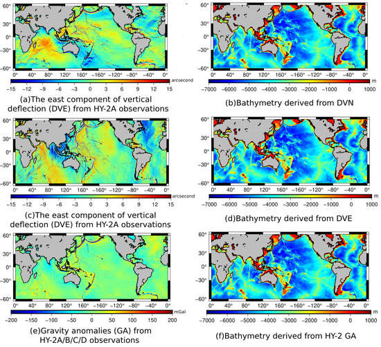
Haiyang-2A (HY-2A), China’s first altimetry satellite mission, was launched more than ten years ago, and its follow-up satellites, HY-2B, HY-2C, and HY-2D, have also been launched. More attention has been paid to the evaluation of these satellite observations in marine gravity field inversion. However, this is not the case for bathymetry inversion. This study is aimed at evaluating the performance of HY-2 gravity field products in bathymetry recovery. Not only gravity anomaly, but also deflection of the vertical from the HY-2 series’ observations is also used. The results show that the bathymetry derived from the deflection of the vertical from HY-2A has a precision of around 128~130 m, and the north-south component performs better than the east-west component. Three versions of the gravity anomaly are used in bathymetry inversion, i.e., HY2ONLY_GRA, WHU16_GRA, and NSOASS22_GRA, and three bathymetry models are derived correspondingly, named as HY2ONLY_BAT, NSOASS22_BAT, and WHU16_BAT, respectively. The results show that HY2ONLY_BAT has a precision of 82.93 m, which is a little poorer than WHU16_BAT; NSOAS22_BAT has the best performance in bathymetry inversion among the three versions of the gravity anomaly. It indicates that HY-2 observations can also contribute to bathymetry inversion compared to current altimetry datasets, since the main difference between WHU16_GRA and NSOASS22_GRA is the use of HY-2 observations. According to spatial analysis results, considerable improvements appear in the west of the Pacific and Indian oceans, and most of the improvements are within 20 m. Meanwhile, the improvements are stronger in the regions with depths ranging between 2600~5500 m. Correlation analysis demonstrates that NSOASS22_BAT is very close to SIO V19.1 and DTU21BAT, which once again indicates the excellent performance of NSOASS22_BAT.

Graphical Abstract

1. Introduction

Bathymetry is significant for economics, the military, and various kinds of scientific investigations. The conventional method usually adopts shipborne sounding equipment to measure water depths. However, it would take 100~200 years and a lot of financial effort to measure the whole of Earth’s ocean depths [1]. With the advancements in satellite altimetry, a more accessible approach has been developed to obtain global bathymetry information, i.e., the inversion based on marine gravity field products [2,3,4]. Several investigators have researched this topic and verified its effectiveness, such as [5,6,7,8,9,10,11,12,13,14]. All these researchers mainly use gravity field products from the Technical University of Denmark (DTU) or Scripps Institution of Oceanography (SIO), such as DTU10GRA, DTU17GRA, SIO V30.1, or SIO V23.1 [5,6,7,8,9,10,11,12,13,14].
Indeed, China has developed its own altimetry satellites, i.e., the Haiyang-2 (HY-2) series [15], including HY-2A, HY-2B, HY-2C, and HY-2D. Observations from HY-2 have been used to derive global marine gravity field products with good performance by several investigators. In [16], a 1′ × 1′ gravity anomaly was developed through the least square collocation method using HY-2A satellite observation data in the South China Sea, and the results show that the HY-2A satellite altimeter has almost identical performance as other Ku band altimeter missions in marine gravity detection. Ref. [17] derived global deflection of the vertical (DV) using HY-2A observations. Their results showed that the differences between HY-2A and EGM2008 have standard deviations of 1.1 s and 3.5 s in the north-south and east-west components of DV, respectively. Ref. [18] verified the excellent performance of HY-2A by comparing the derived DV with XGM2019e-DOV. Ref. [19] systematically evaluated the performance of HY-2 series satellite observations in global marine gravity field recovery, and gravity field products with girds of 1′ × 1′ were derived with high accuracy. Ref. [20] proved that HY-2 had similar accuracy to CryoSat-2 during the same time period. Ref. [21] demonstrated that HY-2 data can improve the precision of the global gravity anomaly by nearly 0.1 mGal.
The above literature indicate that HY-2 performs well in marine gravity field recovery. However, few investigations discuss the performance of these products in global bathymetry inversion. Although [22] evaluated the performance of HY-2A over the Gulf of Guinea, the conclusion is only suitable for that study region but not the global region. Additionally, the work of [22] evaluated the performance of only HY-2A. Indeed, besides HY-2A, HY-2B, HY-2C, and HY-2D can enhance the accuracy of the recovered marine gravity field products [19]. Therefore, it is meaningful to investigate the global performance of the newest HY-2 products, and this study investigates this topic by inverting bathymetry using available HY-2 gravity field products. It should be noted that, this study not only adopted GA data but also HY-2A-derived DV to invert the bathymetry. Section 2 introduces the related data processing method; Section 3 describes the data used in this study; and Section 4 presents the inversion results and analyzes their accuracy. Section 5 and Section 6 give the discussion and conclusions, respectively.

2. Method

2.1. Bathymetry Inversion from GA

GA is generally used to invert the seafloor topography in medium and short wavelength bands (usually 10~200 km) [11,12,23], and the shipborne depths data at control points are often used to build a long-wavelength depth model [24]. In the frequency domain, the Fourier transform relationship between GA and submarine topography can be obtained from the equation as follows [25,26,27]:
F ( Δ g ) = 2 π G Δ ρ e k d n = 1 k n 1 n ! · F ( h n )
where F denotes fast Fourier transform (FFT), and F ( h ) is the FFT of water depths h ; F ( Δ g ) is FFT values of GA; G is gravitational constant; Δ ρ denotes the density contrast between the upper crust and seawater; d is the datum depth; k = k x , k y ; k x = 2 π / λ y ; k y = ( 2 π / λ y ) ; λ x and λ y represent the wavelength in x and y directions, respectively. When only linear term is considered, i.e., n = 1, we can get,
h = F - 1 1 2 π G Δ ρ e k d F ( Δ g )
The main steps of bathymetry inversion are as follows:
1.
Construct long-wavelength water depth h l o n g ( x ) . This is achieved by low-pass filtering of shipborne depths;
2.
Filter Δ g ( x ) using a bandpass filter;
3.
Derive the scale coefficients, denoted as a(x), between submarine topography and gravity anomaly in the inversion band;
4.
Recover the bathymetry as Equation (3).
h p r e d i c t ( x ) = h l o n g ( x ) + a ( x ) Δ g ( x )
The primary data processing is shown in Figure 1.
The filters mentioned in the above process were designed as described in [28]. The high- and low-pass filters are defined in Equations (4) and (5).
w 1 ( k ) = 1 e 1 2 k s 2
w 2 ( k ) = 1 + A k 2 π 4 e 2 k d 1
where s = 2 ln 2 k ; A = λ 4 e 4 π d λ .
The band-pass filter, as shown in Equation (6), is indeed a combination of the high- and low-pass filters.
w = w 1 ( k ) w 2 ( k )
The selection of cutoff wavelengths is usually derived by correlation analysis between GA and submarine topography [29,30]. Based on the experience of the relevant literature, 20~160 km is a typical band range for the inversion of submarine topography [31,32]. Therefore, this paper also uses [20~160] km as the filter passband in bathymetry inversion.

2.2. Bathymetry Inversion from DV

The relationship between the disturbing gravitational potential at sea level and water depth can be expressed as follows [25,26,27]:
F ( U ) = 2 π G Δ ρ e | k | d n = 1 | k | n 2 n ! F h n
where U is the disturbing potential generated by seafloor topography.
If we only consider the first-order term in Equation (7), the following equation can be derived [29]:
h = F 1 γ i 2 π G Δ ρ e k d   k k x F η h = F 1 γ i 2 π G Δ ρ e k d   k k y F ξ
γ is mean gravity anomaly. Because the value of Δ ρ at different locations is different, a constant value cannot yield good inversion results. Therefore, it is obtained through the linear regression between the water depth at control points and GA after the downward continuation from sea level to the reference depth [31]. Its advantage is that there is no need to have an accurate density contrast. To make Equation (8) have a linear relationship, let
η = F 1 F ( η ) γ | k | i k x ξ = F 1 F ( ξ ) γ | k | i k y
The following equation can be derived [29]:
h = F 1 1 2 π G Δ ρ e | k | d F ( η ) h = F 1 1 2 π G Δ ρ e | k | d F ( ξ )
By comparing Equations (10) and (2), it is easy to observe that the forms of the 2 equations are the same. Therefore, the principle and steps of inversion of submarine topography based on DV are consistent with GA.

3. Data

3.1. Shipborne Depth

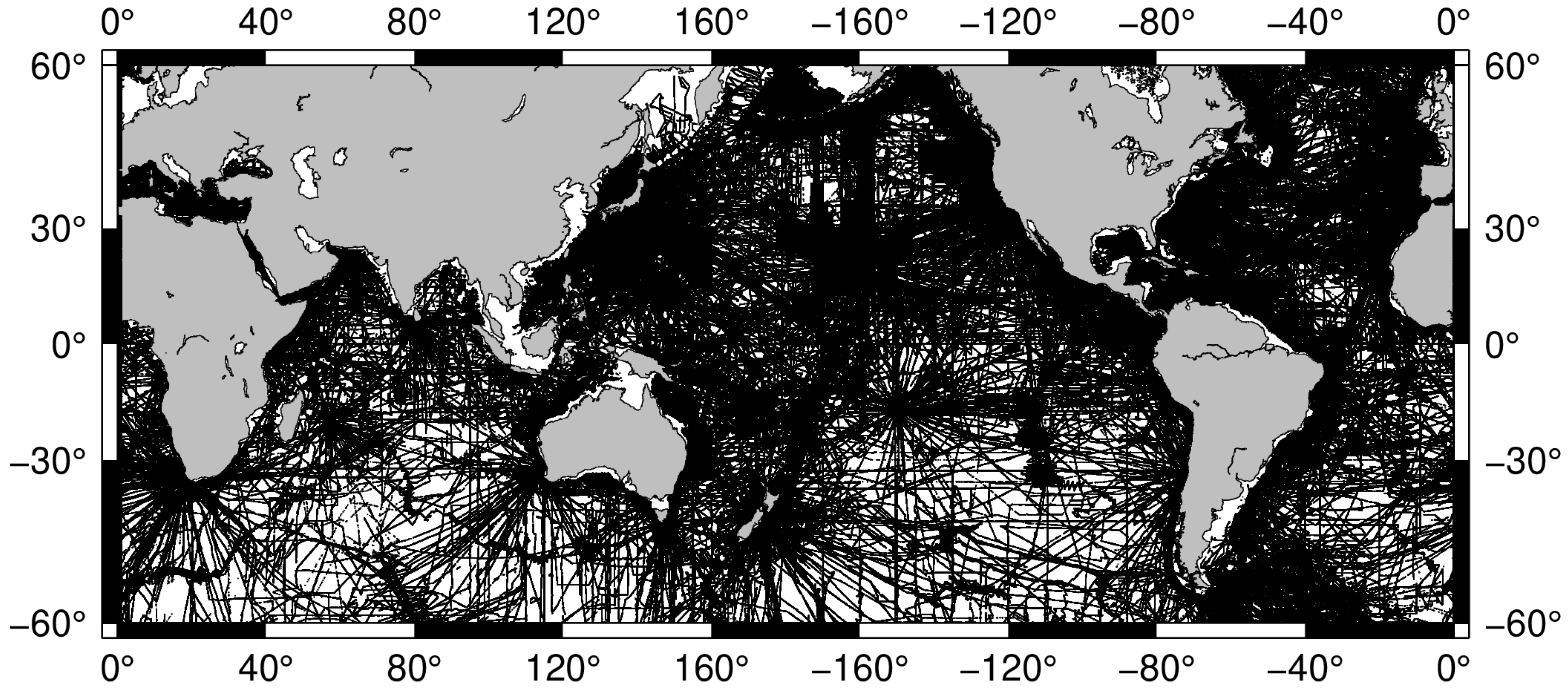
The bathymetric data is from the Geophysical Data Center (https://www.ngdc.noaa.gov/mgg/bathymetry/ (accessed on 24 April 2022)) of the National Oceanic and Atmospheric Administration (NOAA). The number of points is about 66,527,218; the distribution is shown in Figure 2. In the process of inversion, we used ETOPO1 to verify the gross errors of shipborne depths. If the difference between the ship’s bathymetric data and ETOPO1 is greater than 1000 m, the shipborne depth is removed and not used in this study. We removed about 10.8 million points, accounting for 16.3% of the total ship’s bathymetric data. A total of 80% of the remaining data points are used as control points to invert the seabed topography, which is 44581774 points. The remaining 20% is used as test points to evaluate the accuracy of the inversion results, representing 11,145,444 points. In addition, the bathymetric model DTU10BAT provided by DTU (https://ftp.space.dtu.dk/pub/DTU10/, accessed on 24 April 2022) is used to fill in the missing topographic data above the water surface (such as islands) to avoid the adverse effects of bathymetry inversion in such areas.

3.2. Gravity Anomaly

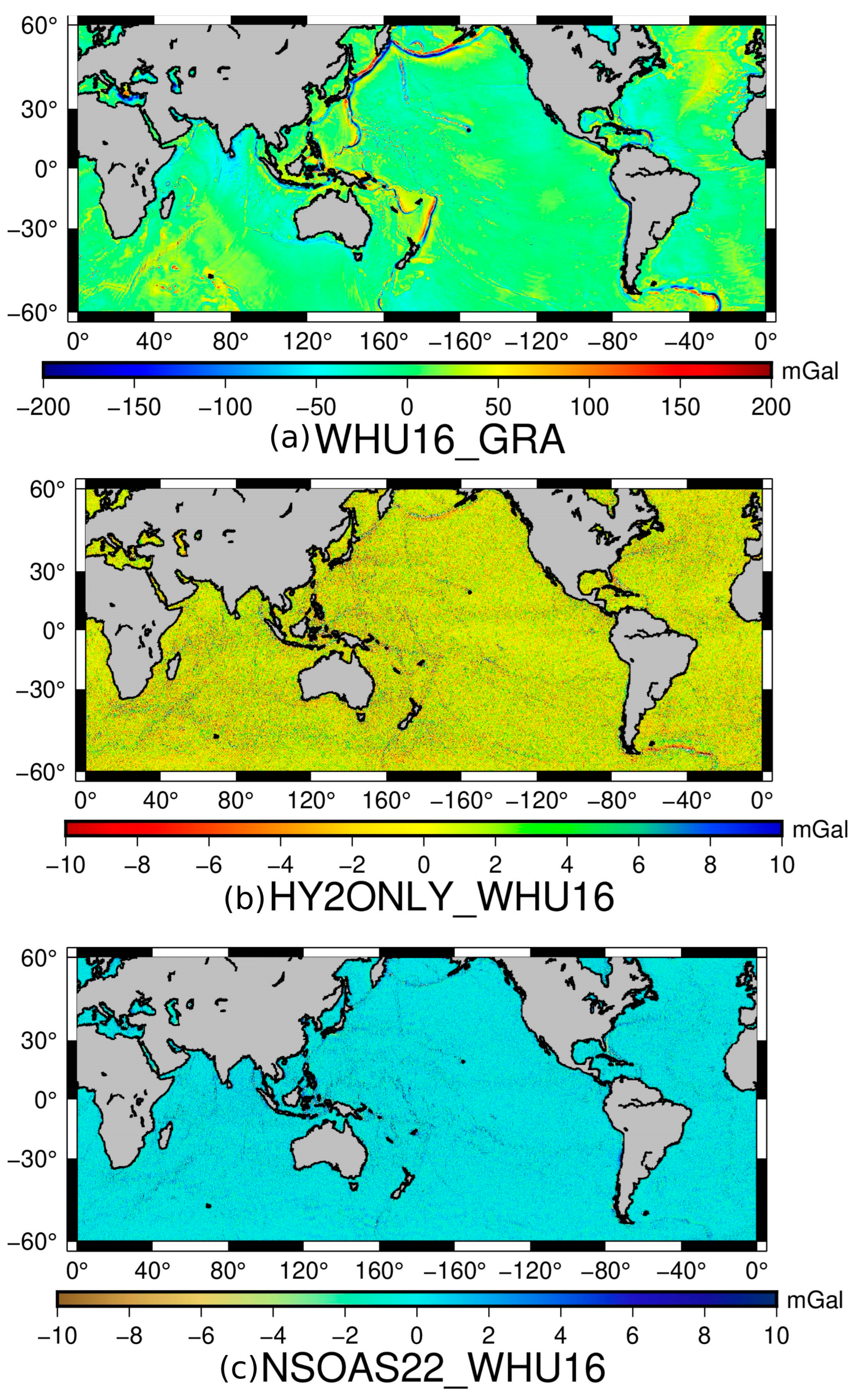
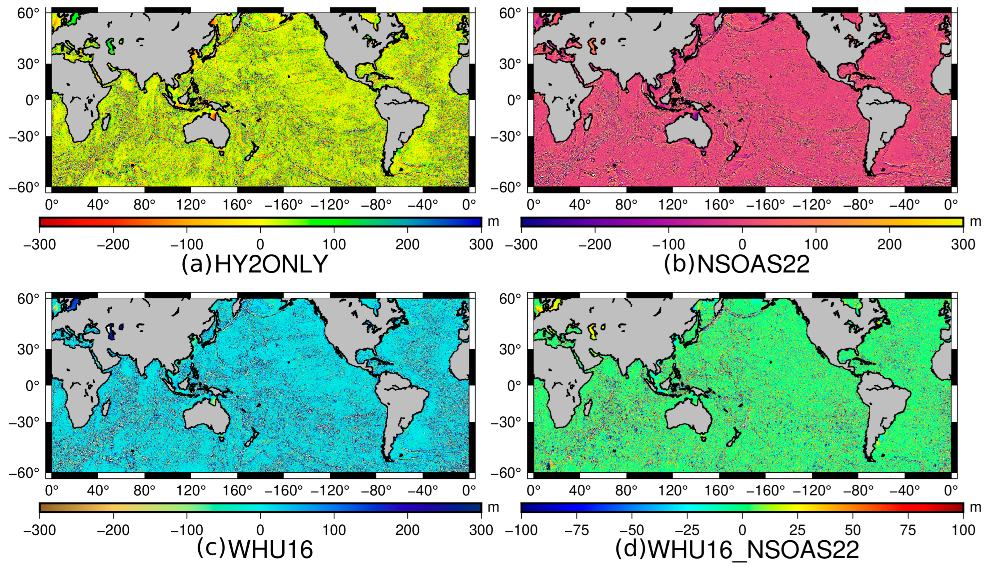
Gravity anomalies used in this study include HY2ONLY_GRA, WHU16_GRA, and NSOAS22_GRA, which are all provided by [19]. HY2ONLY_GRA is derived using pure HY-2 observations; WHU16_ GRA is a gravity anomaly model integrating Geosat, ERS-1, Envisat, Jason-1, Cryosat-2, and SARAL/AltiKa data [19], as shown in Figure 3a; NSOAS22_ GRA is a gravity anomaly model integrating HY-2, Geosat, ERS-1, Envisat, Jason-1, Cryosat-2, and SARAL/AltiKa data [19]. It should be noted that compared to WHU16_ GRA, the main difference of NSOAS22_GRA is the usage of HY-2A, HY-2B, HY-2C, and HY-2D data. The spatial distribution map of NSOAS22_GRA is given in the literature [19], and thus is not shown here. Figure 3b,c show the differences of gravity anomaly between HY2ONLY_GRA and WHU16_GRA, NSOAS22_GRA and WHU16_GRA, respectively. According to [19], the differences between HY2ONLY_GRA, WHU16_GRA, NSOAS22_GRA, and shipborne gravity have standard deviations of 5.6981 mGal, 4.4924 mGal, and 4.3831 mGal, respectively. It indicates that the precision of the GA model NSOAS22_GRA is better than that of the other two GA models.

3.3. Deflection of the Vertical

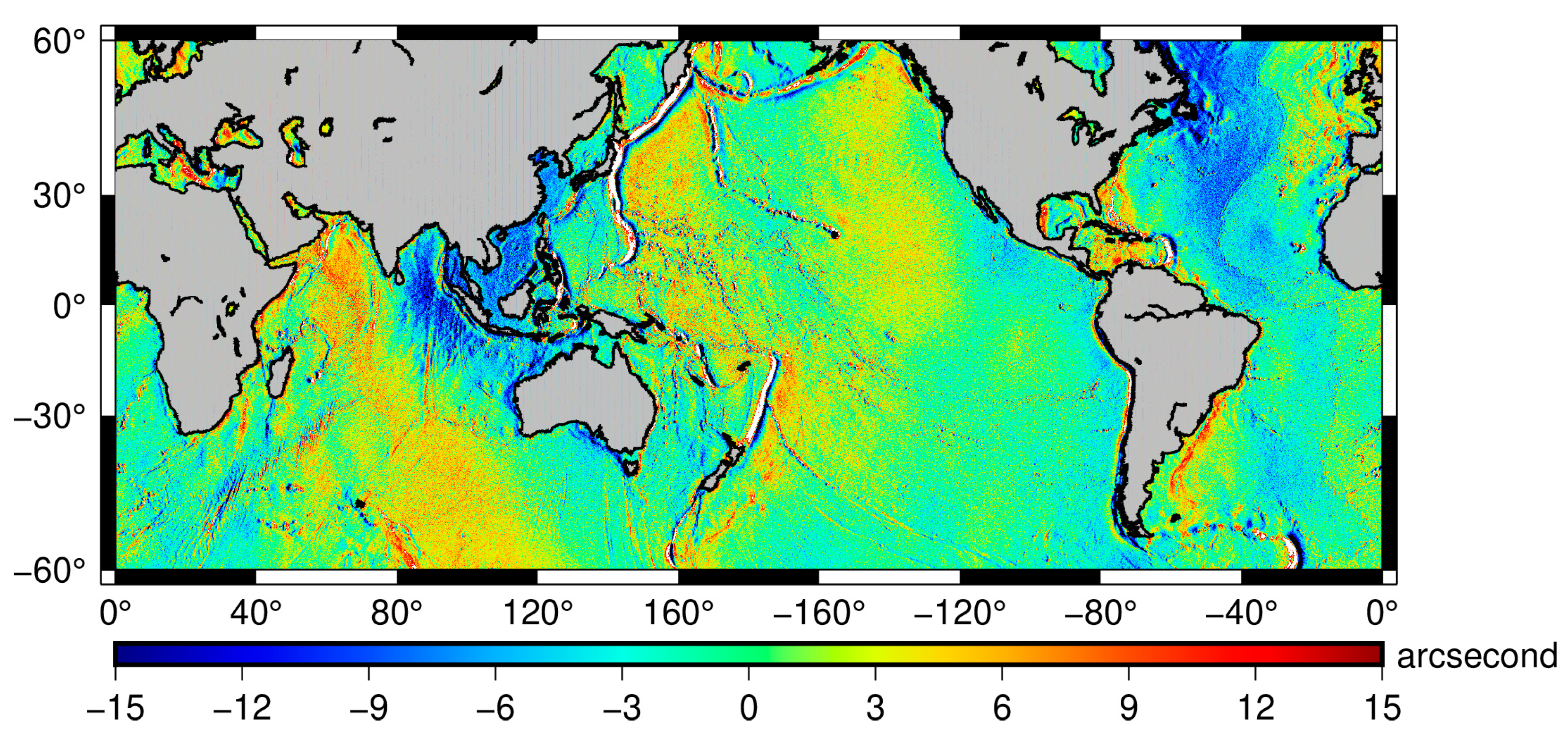
DV with grids of 1′ × 1′ derived by [21] is adopted in this study. The two components are named DOV_N2021 (the north-south component) and DOV_E2021 (the east-west component), respectively. These data are derived from HY-2A observations, and the distributions are given in Figure 4 and Figure 5. According to [21], the differences between DOV_N2021, DOV_E2021, and those of SIO (i.e., SIO_north_31.1 and SIO_east_31.1) have standard deviations of 0.6 and 2.4 arcsec, respectively [21].

4. Results and Analysis

4.1. Results from DV

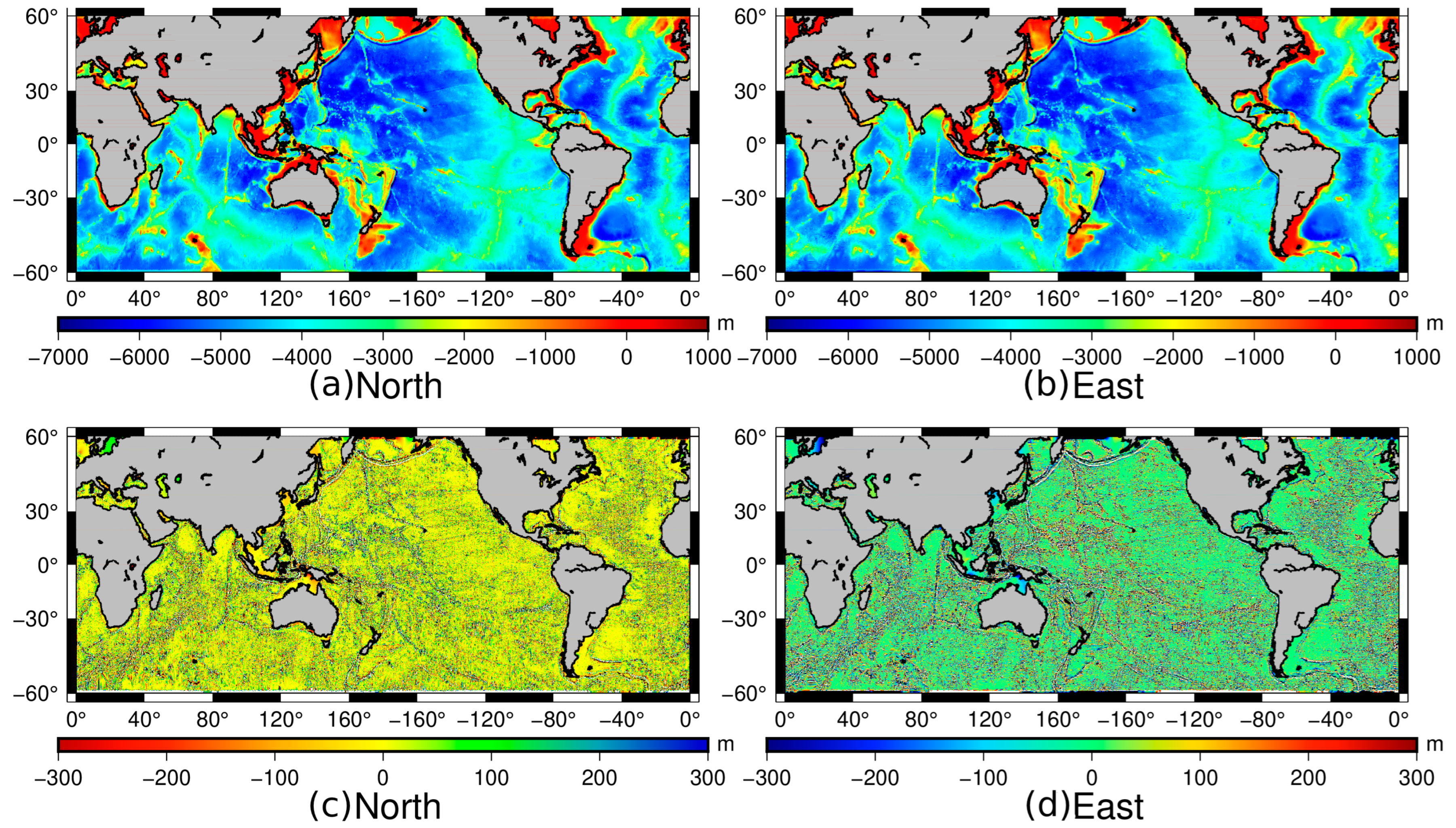
The water depth in the regions with a longitude of 0°~360° and a latitude of −60°~60°N is recovered from DV and named as DOV_N2021BAT and DOV_E2021BAT, respectively. The spatial distribution of the inversion results and the difference between the inversion results and the shipborne depth data are shown in Figure 6. The statistical results of the differences between the shipborne depths and the inversion results at test points are summarized in Table 1.
In Table 1, Removal Ratio means the ratio of the gross error, which is eliminated by using the three STD criteria (i.e., removing the errors that deviate from the mean error by three times the initial STD). The total number is 9,624,310, and the numbers of the removal data are 577,459 and 586,120 for DOV_N2021BAT and DOV_E2021BAT, respectively. According to Figure 6, the bathymetry models constructed by the two components of DV have errors smaller than 100 m in the major region of the study area. According to Table 1, the standard deviations of the inversion results by the north and east components of DV are 128.47 m and 130.27 m, respectively. Table 1 also shows that the inversion result of the north-south component performs better than that of the east-west component, which is consistent with the phenomenon mentioned in the previous section that the accuracy of the east-west component of DV is lower than that of the north-south component [17,21].

4.2. Results from GA

4.2.1. Precision Evaluation

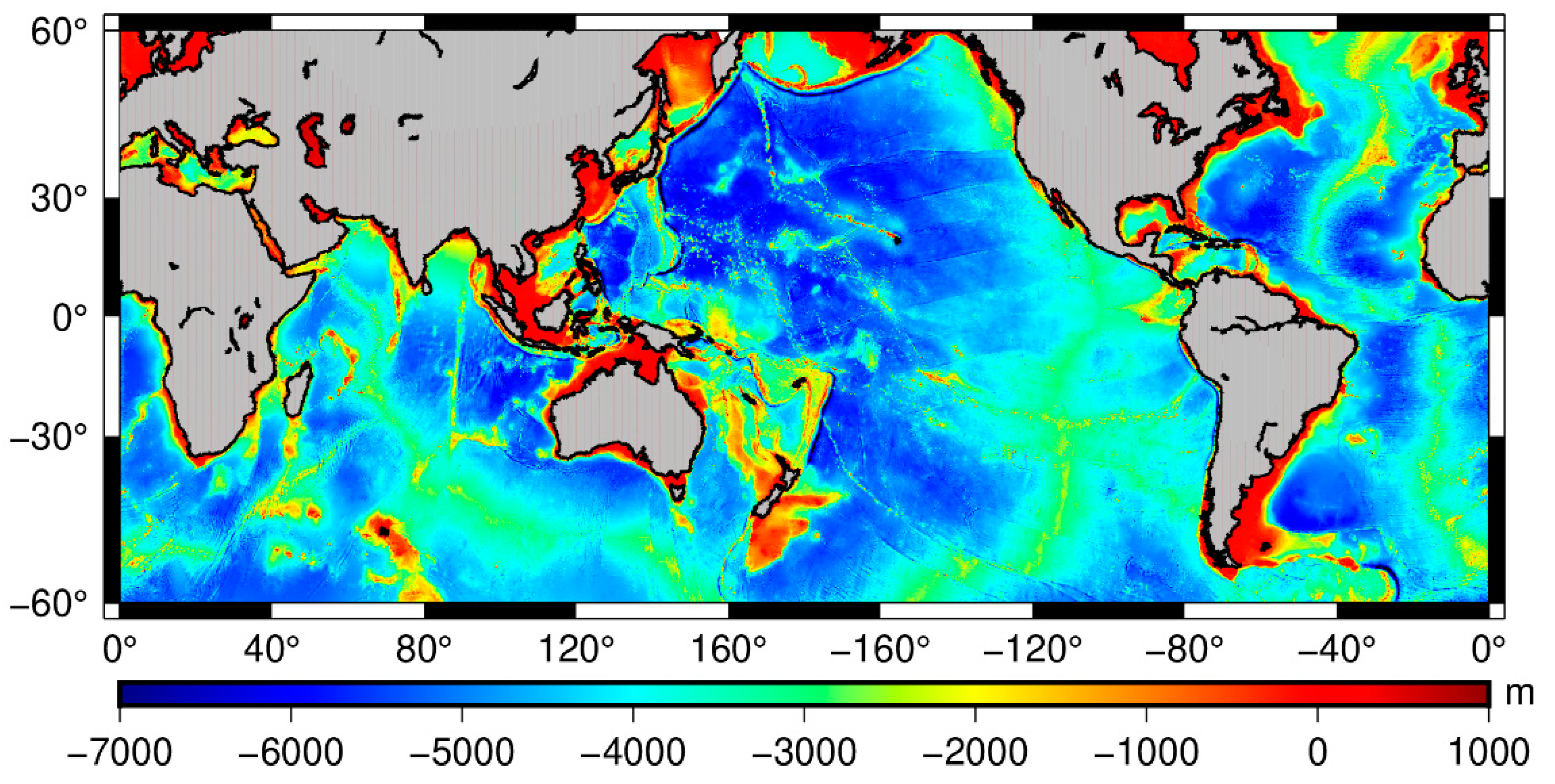
Three global marine bathymetry models are derived for the regions with longitude of 0°~360° and latitude of −60°~60°N using the three groups of GA. We name these three bathymetry models HY2ONLY_BAT, WHU16_BAT, and NSOAS22_BAT, which correspond to HY2ONLY_GRA, WHU_GRA, and NSOAS22_GRA, respectively. Figure 7 shows the spatial distribution of the HY2ONLY_BAT. Since the NSOAS22_BAT and WHU16_BAT are almost the same as HY2ONLY_BAT, as shown in Figure 7, the spatial distributions of them are not presented here. Instead, statistics on the differences between all the bathymetry results and shipborne depths at test points are summarized in Table 2. It needs to be noted that the statistics are only conducted at depths deeper than 1000 m. This is because the bathymetry inversion from gravity field products usually has poorer accuracy in shallow ocean regions [33].
According to Table 2, the precision of bathymetry models retrieved from NSOAS22_GRA performs best among the three derived models, indicating the high accuracy of GA of NSOAS22_GRA. It must be noted that any gross error would influence the statistical results, even though it represents a minor ratio in the data. The largest errors exceed 3000 m according to Table 2 and these can be seen as gross errors. The three STD criteria is used to reduce the impact of gross errors, and we performed this process twice. The total number before gross error removal was 9,624,310; and the numbers of removed data points are 496,614, 512,976, and 496,614 for HY2ONLY_BAT, NSOAS22_BAT, and WHU16_BAT, respectively. The new results are shown in Table 3. It is found that the precisions of the three bathymetry models are all better than 90 m, and NSOAS22_BAT performs best. Since, compared to WHU16_GRA, the main difference of NSOASS_GRA is the usage of HY-2 observations, the above results prove that HY-2 data is beneficial in improving the accuracy of the submarine terrain inversion.
We also compared our derived results with DTU21BAT grid data (https://ftp.space.dtu.dk/pub/DTU21/, accessed on 6 December 2022), and the statistics of the comparisons are presented in Table 4. The total number before gross error removal was 102,985,566, and the numbers of the removed data points in gross error processing are 4,394,817, 4,738,425, and 4,850,971 for HY2ONLY_BAT, NSOAS22_BAT, and WHU16_BAT, respectively. According to Table 4, the mean differences between the inversion model and DTU21BAT model are 12.93 m, 12.35 m, and 12.52 m, respectively, and the standard deviations are 135.76 m, 125.59 m, and 126.20 m, respectively. It is found that the standard deviation of the difference between the NSOAS22 model and the DTU21BAT model is the smallest. NSOAS22_BAT was then compared with the SIO V19.1 model (https://topex.ucsd.edu/pub/, accessed on 24 April 2022), and the results are shown in Table 5. The total number was around 103 million, and the number of the removed data in gross error processing are 3,966,397 and 3,955,816 for the comparisons between NSOA22_BAT, DTU21BAT, and the SIO V19.1 model, respectively. According to this table, the mean difference between NSOAS22_BAT and the SIO model is 17.00 m, and the standard deviation is 122.21 m.
To further analyze the consistency between NOSASS22_BAT, SIO V19.1, and DTU21BAT, the correlation between them is calculated. The results show that the correlations between NOSASS22_BAT and SIO V19.1, DTU21BAT are 0.9907 and 0.9894, respectively. We also found that DTU21BAT and SIO V19.1 have a very high correlation, i.e., 0.9970. All these results show that these three models have similar precision since they are close to each other.

4.2.2. Spatial Distribution of the Errors

To analyze the spatial distribution of the errors, Figure 8 presents the differences between the derived bathymetry models and shipborne depth data. To present the contribution of HY-2, differences in the inversion error between WHU16_BAT and NSOASS22 are also shown in Figure 8.
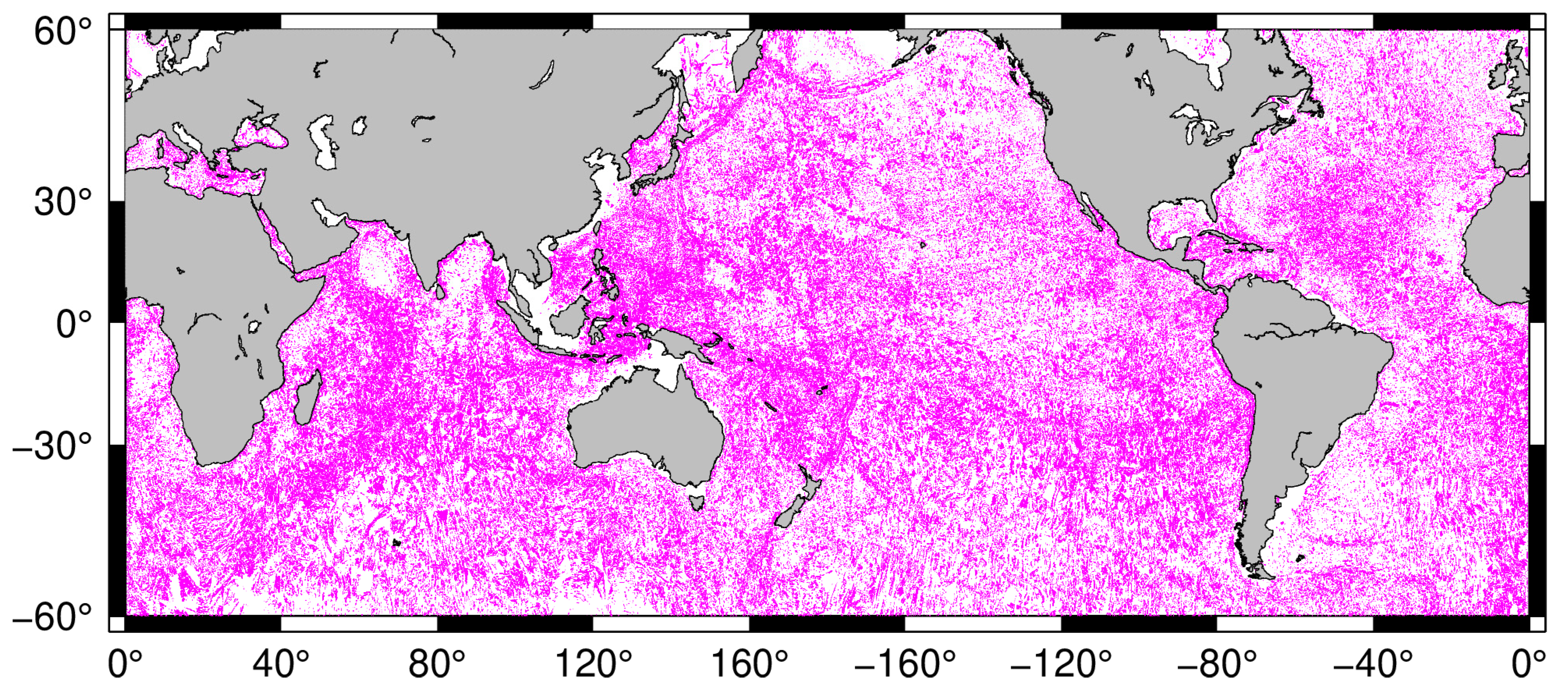
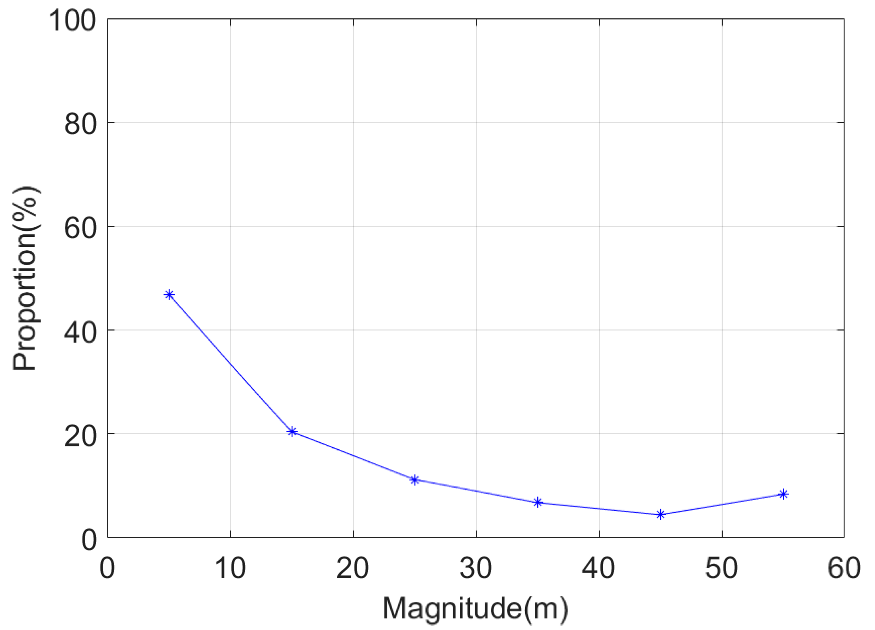
According to Figure 8, all the bathymetry models exhibited significant errors in the southwest region of the Indian Ocean and smaller noises over the northeast regions of the Pacific Ocean. This point is also substantiated in Figure 9, which shows the point positions with accuracy improvements larger than 50 m. According to Figure 8d, the differences between NSOAS22_GRA and WHU16_GRA derived results have magnitudes smaller than 25 m in the major regions. According to Figure 9, considerable improvements appear in the west of the Pacific and Indian oceans. Figure 10 shows the ratio of the points with different improvements. According to Figure 10, the accuracy improvement accounts for 46.28% in the range of 0~10 m and 20.37% in the range of 10~20 m. It is found that nearly 10% of the points are improved with a magnitude exceeding 50 m. This means HY-2A can contribute a lot in the related regions (see Figure 9).

4.2.3. Analysis on Accuracy Variation with Water Depths

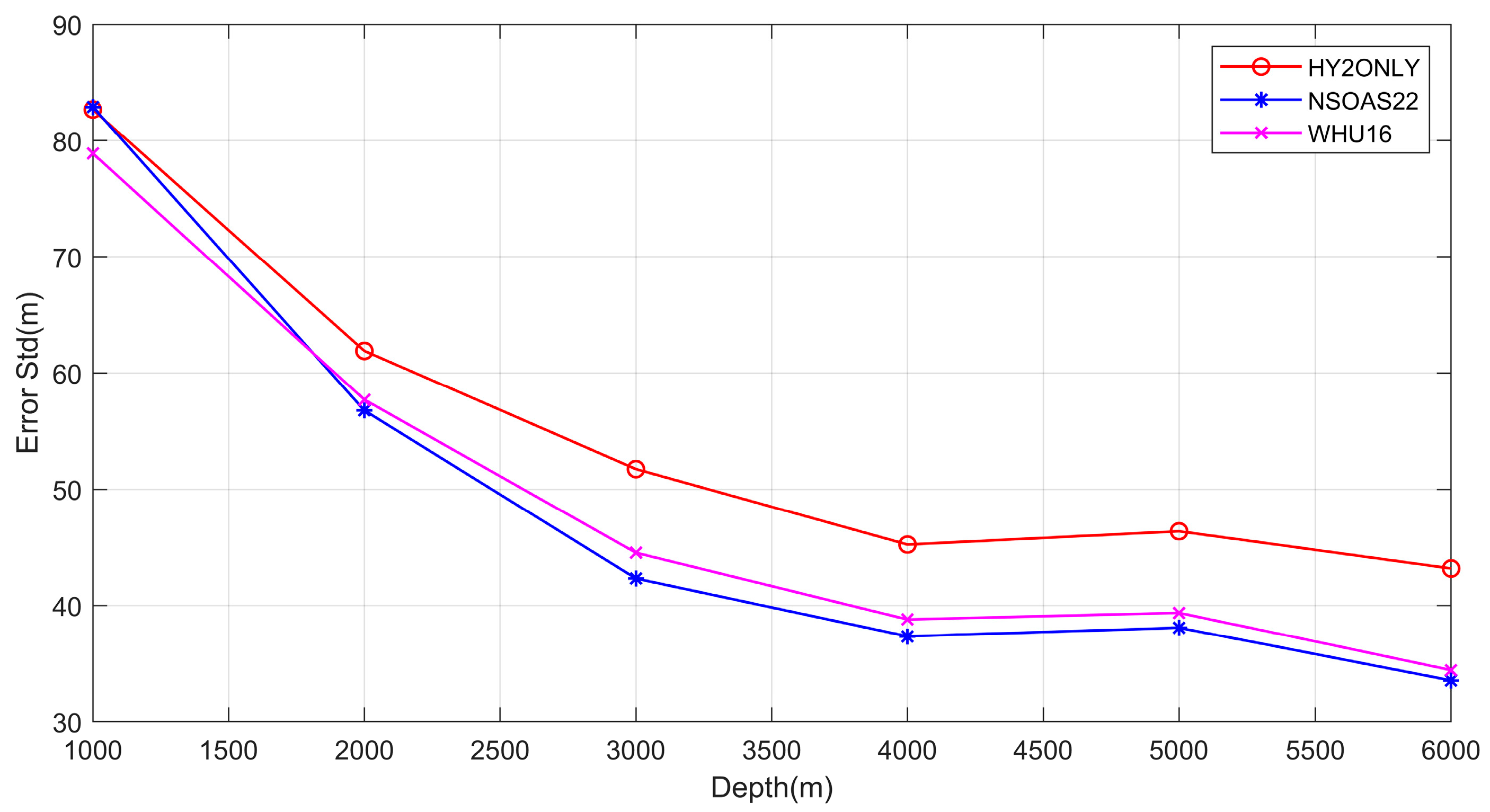
To analyze the variation in accuracy with water depths, statistics are conducted for different water depths. 1000 m is selected as the interval. Error STD variations are shown in Figure 11. It can be found that the error STD of the three inversion models gradually decreases with an increase in water depth, indicating that the deeper the ocean, the better the inversion accuracy is. Moreover, the error STD of the NSOAS22_BAT is lower than that of the WHU16_BAT in the range of 2000~6000 m water depth, which proves that the integration of HY-2 data can improve the bathymetry in regions with these water depths. However, in regions with depths shallower than 1500 m, the inversions from HY2ONLY_GRA and NSOAS22_GRA perform a little worse than WHU16_GRA. This reason would be investigated in future research.

4.2.4. Accuracy Variation with Wavelength

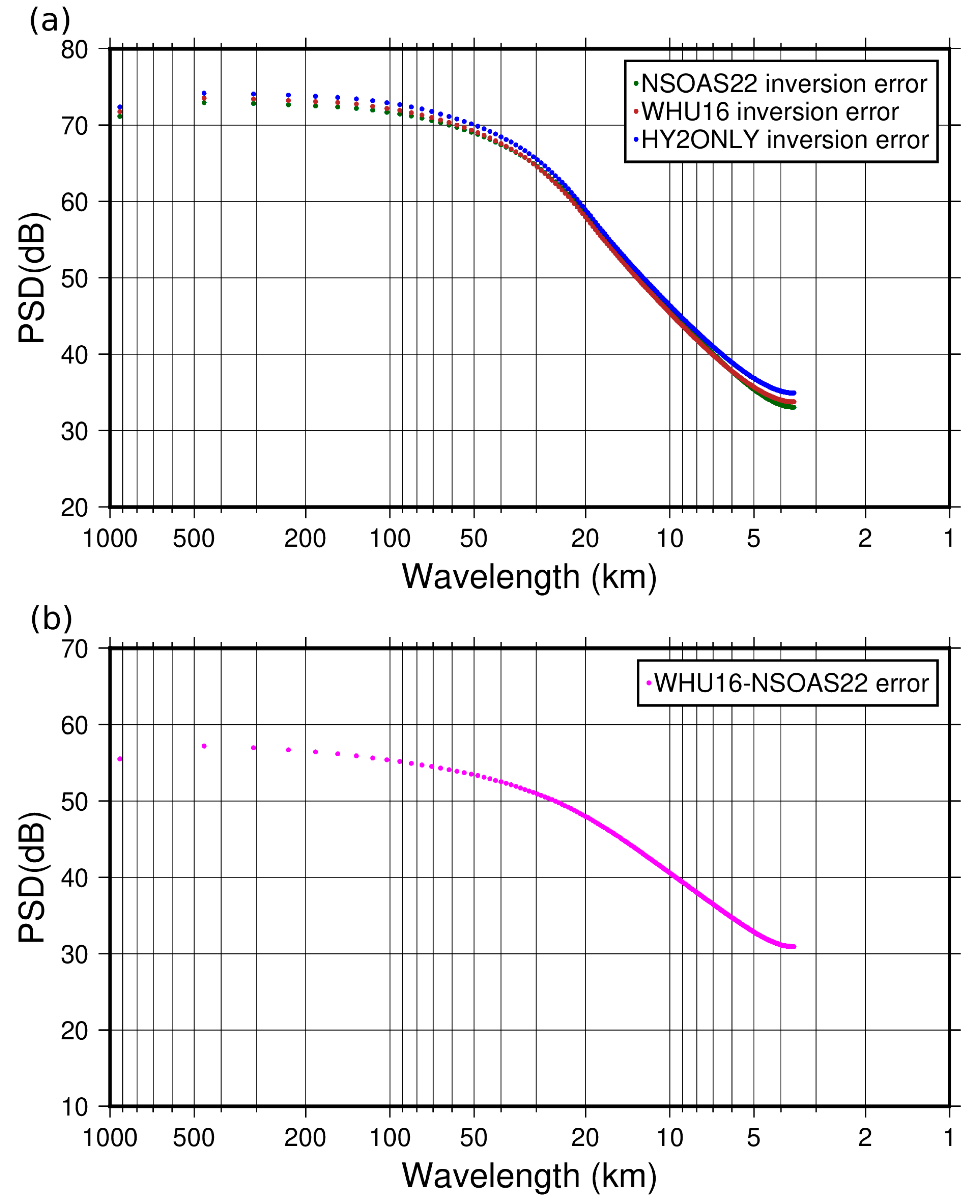
To verify the contribution of HY-2 in terms of wavelengths of bathymetry, Figure 12 presents the error PSD of the inversion results. It can be seen from Figure 12a that when the wavelength is smaller than 20 km, the errors of NSOAS22_BAT and WHU16_BAT have almost the same magnitude, both of which are a little lower than HY2ONLY_BAT. When the wavelength is greater than 20 km, the NSOAS22_BAT performs a little better than the other two models. Figure 12b demonstrates the error differences between the WHU16_BAT and the NSOASS22_BAT, i.e., the errors of the WHU16_BAT minus the errors of the NSOAS22_BAT. Figure 12b indicates that HY-2 data can contribute more to the long-wavelength part of bathymetry.

5. Discussion

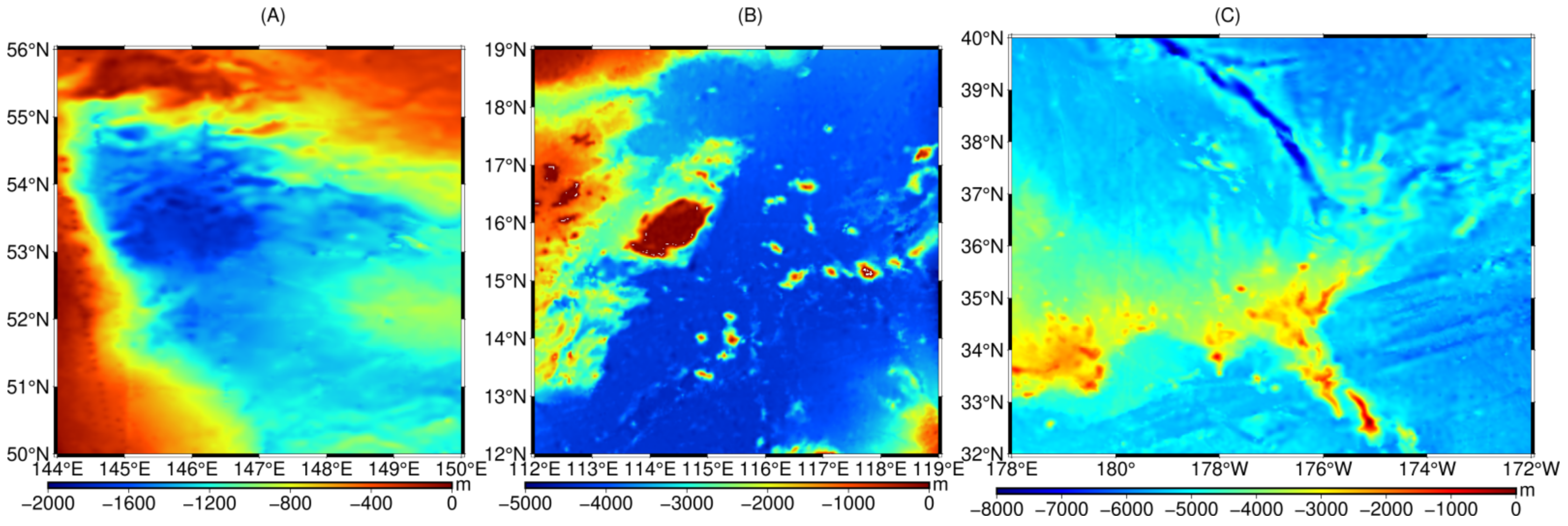
The above bathymetry inversion only considers the linear relationship between seabed topography and gravity field information. However, non-linear terms exist (see Equations (1) and (7)). The literature [34,35] mentioned that the non-linear effect has an impact on the bathymetry inversion accuracy, but the improvement for the whole global ocean would not be strong [11]. Therefore, this study only discusses this issue in local regions. To analyze the impact of the non-linear terms on different ocean regions, three test regions are selected, i.e., A, B, and C (see Figure 13). Among them, region A is located in 144°~150°E, 50°~56°N, and the variation range of water depth is 0~2000 m. Region B is located in 112°~119°E, 12°~20°N, and the variation range of water depth is 0~5000 m. Region C is located in 178°~188°E, 32°~40°N, and the variation range of water depth is 0~8000 m. In this section, the GA data is taken from NSOASS22_GRA. The reason for choosing these three regions is that they represent different types of topographic relief, such as different mean depths.
To evaluate the non-linear term impact, we consider the first three terms in Equation (1), i.e., n = 3 , and then Equation (1) becomes:
F ( Δ g ( k ) ) = 2 π G Δ ρ e k d F ( h ( k ) ) + 2 π G Δ ρ e k d 1 2 k F ( h 2 ( k ) ) + 1 6 k 2 F ( h 3 ( k ) )
To remove the non-linear effect, we adopted the initially derived bathymetry information to forward model the GA effect caused by high order terms, i.e., the following term,
F ( Δ g ( k ) ) = 2 π G Δ ρ e k d 1 2 k F ( h 2 ( k ) ) + 1 6 k 2 F ( h 3 ( k ) )
And then removed it from the total GA data. The newly obtained GA data is then used to derive a new bathymetry model. In this Section, SIO V19.1 model data is adopted for error evaluation, and the results are shown in Table 6. It needs to be noted that errors exceeding 1000 m are removed to reduce the impact of gross errors. The results show that the bathymetry inversion accuracy is improved by considering the non-linear effects, with magnitudes of 0.05 m, 1.69 m, and 0.88 m in terms of STD, respectively, in regions A, B, and C.
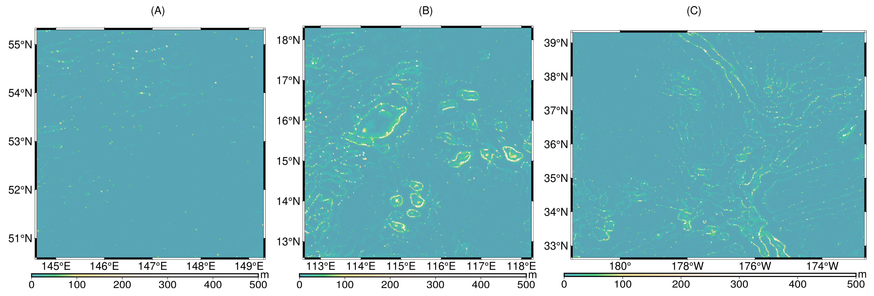
To show the improvement with variation in locations, the absolute differences between the initial and new bathymetry models are presented in Figure 14. This figure demonstrates that the differences in regions B and C are stronger than those in region A. For example, there are more locations where the differences exceed 100 m in Figure 14B,C than in Figure 14A. Comparing Figure 14B,C and Figure 13B,C, we can conclude that the non-linear effects are relatively stronger in the areas with significant variations in submarine topographic relief, which should be considered in the related regions. One possible method is to first inverse bathymetry without considering non-linear terms, and then evaluate the characteristics of bathymetry. If the bathymetry varies greatly, one can inverse the bathymetry again using the gravity anomaly after removing the non-linear effect using Equation (12).

6. Conclusions

In this study, the performance of HY-2-derived gravity field products, including DV and GA, in bathymetry inversion is evaluated. The results show that the DV from HY-2A can be used to derive bathymetry with an error standard deviation of around 130 m. The north-south component performs better than the east-west one. Bathymetry derived from HY2ONLY_GRA, i.e., HY2ONLY_BAT, has an error standard deviation of around 85 m, which is a little worse than that of WHU16_GRA, which is derived from multi-satellite altimetry observations. The bathymetry from NSOAS22_GRA performs best among the three versions of gravity anomaly inversion results. When compared to WHU16_GRA, the main difference of NSOAS22_GRA is the usage of HY-2 data. Thus, the improvements of NSOAS22_BAT compared to WHU16_BAT are due to the contribution of HY-2 data. Analysis showed that by using HY-2 data, in more than 50% of locations where the accuracy is improved, the accuracy improvement exceeds 10 m (see Figure 10). In addition, according to precision analysis, NSOAS22_BAT has a comparable precision with SIO V19.1 and DTU21BAT. This once again substantiates the contribution of HY-2 data.
Tests on non-linear effects show that the greater the fluctuation of submarine terrain, the greater the impact of the non-linear effect on the accuracy of bathymetry inversion. In some local regions, the maximum improvement after considering the non-linear effect exceeded 100 m, indicating that the non-linear effect should be considered in the related regions. It should also be noted that, although HY-2-derived products can be used to derive global bathymetry, limitations still exist. Examples are the low accuracy for the shallow ocean region, and the limited sensitive wavelength of gravity field products for bathymetry inversion. Because of these, more different types of datasets, such as satellite imagery and gravity gradient data; and different inversion methods, such as the deep learning method [14] are needed to improve the bathymetry accuracy.

Author Contributions

Conceptualization, X.W. and Y.J.; methodology, X.W.; software, X.W., H.W. and W.M.; investigation, all the authors; resources, X.W. and Y.J.; data curation, X.W. and H.W.; writing—original draft preparation, X.W. and H.W.; writing—review and editing, all the authors; funding acquisition, X.W. and Y.J. All authors have read and agreed to the published version of the manuscript.

Funding

This study was supported by the National Natural Science Foundation of China (No. 42074017, 42204009).

Data Availability Statement

The shipborne data can be downloaded from: https://www.ngdc.noaa.gov/mgg/bathymetry/ (accessed on 24 April 2022). Gravity anomaly data is downloaded from: https://pan.baidu.com/s/14vfqMYpBMSi6VrRlPZWbPw?pwd=5u05 (accessed on 16 September 2022); Deflection of the vertical can be obtained from the corresponding author.

Acknowledgments

The authors would like to thank NOAA for providing shipborne depth data and Shengjun Zhang for providing gravity anomaly data. We also would like to thank Annan. R.F for the language help.

Conflicts of Interest

The authors declare no conflict of interest.

References

  1. Sandwell, D.T.; Smith, W.H.F.; Gille, S.; Jayne, S.; Soofi, K.; Coakley, B. Bathymetry from Space: White Paper in Support of a High-Resolution, Ocean Altimeter Mission; Scripps Institution of Oceanography: San Diego, CA, USA, 2001; pp. 1–54. [Google Scholar]
  2. Sandwell, D.T.; Smith, W.H.F. Marine gravity anomaly from Geosat and ERS 1 satellite altimetry. J. Geophys. Res. 1997, 102, 10039–10054. [Google Scholar] [CrossRef] [Green Version]
  3. Yang, J. Seafloor topography estimation from gravity gradients. Acta Geod. Cartogr. Sin. 2021, 50, 708. [Google Scholar] [CrossRef]
  4. Ouyang, M.; Sun, Z.; Zhai, Z.; Liu, X. Bathymetry Prediction Based on the Admittance Theory of Gravity Anomalies. Acta Geod. Cartogr. Sin. 2015, 44, 1092–1099. [Google Scholar] [CrossRef]
  5. Hwang, C. A bathymetric model for the south China Sea from altimetry and depth data. Mar. Geod. 1999, 22, 37–51. [Google Scholar] [CrossRef]
  6. Kim, J.W.; von Frese, R.R.B.; Lee, B.Y.; Roman, D.R.; Doh, S.-J. Altimetry-derived gravity predictions of bathymetry by the gravity-geologic method. Pure Appl. Geophys. 2011, 168, 815–826. [Google Scholar] [CrossRef]
  7. Hsiao, Y.S.; Hwang, C.; Cheng, Y.S.; Chen, L.C.; Hsu, H.J. High-resolution depth and coastline over major atolls of South China Sea from satellite altimetry and imagery. Remote Sens. Environ. 2016, 176, 69–83. [Google Scholar] [CrossRef]
  8. Yang, J.; Jekeli, C.; Liu, L. Seafoor topography estimation from gravity gradients using simulated annealing. J. Geophys. Res. Solid Earth 2018, 123, 6958–6975. [Google Scholar] [CrossRef]
  9. Fan, D.; Li, S.; Meng, S.; Xing, Z.; Li, X.; Feng, J. Submarine topography model of South China Sea based on admittance function. Surv. Mapp. Sci. 2018, 43, 44–49. [Google Scholar] [CrossRef]
  10. Tozer, B.; Sandwell, D.T.; Smith, W.H.F.; Olson, C.; Beale, J.; Wessel, P. Global bathymetry and topography at 15 arc seconds: SRTM15+. Earth Space Sci. 2019, 6, 1847–1864. [Google Scholar] [CrossRef]
  11. Hu, M.; Zhang, S.; Jin, T.; Wen, H.; Chu, Y.; Jiang, W.; Li, J. A new global seafloor terrain model BAT_WHU2020. Acta Geod. Cartogr. Sin. 2020, 49, 939–954. [Google Scholar]
  12. Hu, M.; Jin, T.; Jiang, W.; Chu, Y.; Wen, H.; Li, J. Bathymetry Model in the Northwestern Pacific Ocean Predicted from Satellite Altimetric Vertical Gravity Gradient Anomalies and Ship-Board Depths. Mar. Geod. 2021, 45, 24–46. [Google Scholar] [CrossRef]
  13. Sui, X.; Zhang, R.; Wan, X.; Li, Y. Inversion and analysis of seafloor topography based on satellite altimeter data. Spacecr. Eng. 2017, 26, 130–136. [Google Scholar]
  14. Annan, R.F.; Wan, X. Recovering Bathymetry of the Gulf of Guinea Using Altimetry-Derived Gravity Field Products Combined via Convolutional Neural Network. Surv. Geophys. 2022, 43, 1541–1561. [Google Scholar] [CrossRef]
  15. Peng, H.; Lin, M.; Mu, B.; Zhou, W. Global statistical evaluation and quality analysis of HY-2A satellite radar altimeter data. Acta Oceanol. Sin. 2015, 37, 54–66. [Google Scholar]
  16. Zhu, C.; Guo, J.; Hwang, C.; Gao, J.; Yuan, J.; Liu, X. How HY-2A/GM altimeter performs in marine gravity derivation: Assessment in the South China Sea. Geophys. J. Int. 2019, 219, 1056–1064. [Google Scholar] [CrossRef]
  17. Wan, X.; Annan, R.F.; Jin, S.; Gong, X. Vertical Deflections and Gravity Disturbances Derived from HY-2A Data. Remote Sens. 2020, 12, 2287. [Google Scholar] [CrossRef]
  18. Ji, H.; Guo, J.; Zhu, C.; Yuan, J.; Liu, X.; Li, G. On Deflections of Vertical Determined From HY-2A/GM Altimetry Data in the Bay of Bengal. IEEE J. Sel. Top. Appl. Earth Obs. Remote Sens. 2021, 14, 12048–12060. [Google Scholar] [CrossRef]
  19. Zhang, S.; Zhou, R.; Jia, Y.; Jin, T.; Kong, X. Performance of HaiYang-2 altimetric data in marine gravity research and a new global marine gravity model NSOAS22. Remote Sens. 2022, 14, 4322. [Google Scholar] [CrossRef]
  20. Guo, J.; Luo, H.; Zhu, C.; Ji, H.; Li, G.; Liu, X. Accuracy comparison of marine gravity derived from HY-2A/GM and CryoSat-2 altimetry data: A case study in the Gulf of Mexico. Geophys. J. Int. 2022, 230, 1267–1279. [Google Scholar] [CrossRef]
  21. Wan, X.; Hao, R.; Jia, Y.; Wu, X.; Wang, Y.; Feng, L. Global marine gravity anomalies from multi-satellite altimeter data. Earth Planets Space 2022, 74, 165. [Google Scholar] [CrossRef]
  22. Wan, X.; Annan, R.F.; Wang, W. Assessment of HY-2A GM data by deriving the gravity field and bathymetry over the Gulf of Guinea. Earth Planets Space 2020, 72, 151. [Google Scholar] [CrossRef]
  23. Wan, X.; Ran, J.; Jin, S. Sensitivity analysis of gravity anomalies and vertical gravity gradient data for bathymetry inversion. Mar. Geophys. Res. 2019, 40, 87–96. [Google Scholar] [CrossRef]
  24. Xiang, X.; Wan, X.; Zhang, R.; Li, Y.; Sui, X.; Wang, W. Bathymetry Inversion with the Gravity-Geologic Method: A Study of Long-Wavelength Gravity Modeling Based on Adaptive Mesh. Mar. Geod. 2017, 40, 329–340. [Google Scholar] [CrossRef]
  25. Parker, R.L. 1972, The rapid calculation of potential anomalies. J. Geophys. R. 1972, 31, 447–455. [Google Scholar]
  26. Hu, M.; Li, J.; Li, H.; Xing, L. Bathymetry Predicted from Vertical Gravity Gradient Anomalies and Ship Soundings. Geod. Geodyn. 2014, 5, 41–46. [Google Scholar] [CrossRef] [Green Version]
  27. Hu, M.; Li, J.; Li, H.; Shen, C.; Jin, T.; Xing, L. Predicting Global Seafloor Topography Using Multi-Source Data. Mar. Geod. 2015, 38, 176–189. [Google Scholar] [CrossRef]
  28. Smith, W.H.F.; Sandwell, D.T. Bathymetric prediction from dense satellite altimetry and sparse shipboard bathymetry. J. Geophys. Res. 1994, 99, 21803–21824. [Google Scholar] [CrossRef]
  29. Wan, X.; Liu, B.; Sui, X.; Annan, R.F.; Hao, R.; Min, Y. Bathymetry inversion using the deflection of the vertical: A case study in South China Sea. Geod. Geodyn. 2022, 13, 492–502. [Google Scholar] [CrossRef]
  30. Marks, K.M.; Smith, W.H.F. Radially symmetric coherence between satellite gravity and multibeam bathymetry grids. Mar. Geophys. Res. 2012, 33, 223–227. [Google Scholar] [CrossRef]
  31. Hu, M.; Li, J.; Xing, L. Inversion of global seafloor topographic model from vertical gravity gradient anomalies. J. Surv. Mapp. 2014, 43, 558–565, +574. [Google Scholar] [CrossRef]
  32. Fan, D.; Li, S.; Meng, S.; Xing, Z.; Feng, J.; Zhang, C. Inversion of seafloor topography in the Philippine Sea area using combined multi-source gravity data. J. Surv. Mapp. 2018, 47, 1307–1315. [Google Scholar]
  33. Fan, D.; Li, S.; Meng, S.; Xing, Z.; Zhang, C.; Feng, J. Comparison and analysis on seafloor topography inversion methods with different isostatic compensation models. J. Chin. Inert. Technol. 2019, 27, 51–59. [Google Scholar]
  34. Fan, D.; Li, S.; Ouyang, Y.; Meng, S.; Chen, C.; Xing, Z.; Zhang, C. Least squares collocation inversion method considering the nonlinear term of seabed topography. J. Surv. Mapp. 2021, 50, 953–971. [Google Scholar]
  35. Fan, D.; Li, S.; Meng, S.; Xing, Z.; Zhang, C.; Feng, J.; Qu, Z. Influence Analysis of High-order Seafloor Topography on Sea Surface Gravity Information. Geomat. Inf. Sci. Wuhan Univ. 2021, 46, 1328–1335. [Google Scholar] [CrossRef]
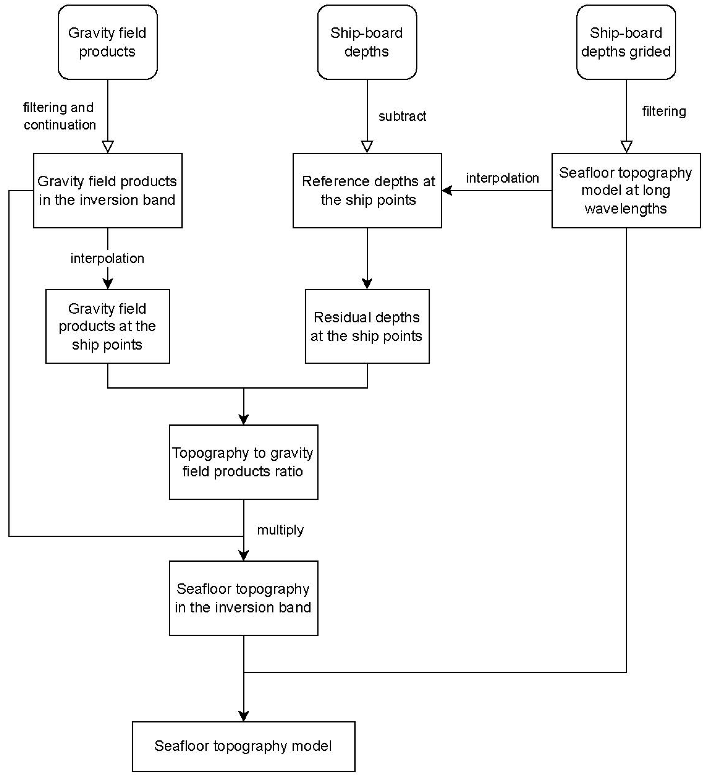
Figure 1. Data processing flow chart for bathymetry inversion.
Remotesensing 15 00032 g001
Figure 2. Distribution of ship survey routes.
Remotesensing 15 00032 g002
Figure 3. Gravity anomaly: (a) WHU16_GRA; (b) The difference between HY2ONLY_GRA and WHU16_GRA; and (c) The difference between NSOAS22_GRA and WHU16_GRA.
Remotesensing 15 00032 g003
Figure 4. DOV_N2021.
Remotesensing 15 00032 g004
Figure 5. DOV_E2021.
Remotesensing 15 00032 g005
Figure 6. (a) The spatial distribution of DOV_N2021BAT; (b) The spatial distribution of DOV_E2021BAT; (c) The differences between DOV_N2021BAT and shipborne depths; (d) The differences between DOV_E2021BAT and shipborne depths.
Remotesensing 15 00032 g006
Figure 7. Global bathymetry model HY2ONLY_BAT.
Remotesensing 15 00032 g007
Figure 8. Error distribution of (a) HY2ONLY_BAT, (b) NSOAS22_BAT, (c) WHU16_BAT, and (d) the absolute error differences between WHU16_BAT and NSOASS22_BAT (WHU16_BAT absolute error minus that of NSOASS22_BAT).
Remotesensing 15 00032 g008
Figure 9. Positions of the points with an improvement greater than 50 m.
Remotesensing 15 00032 g009
Figure 10. Points proportion with an improvement of 0~10 m, 10~20 m, 20~30 m, 30~40 m, 40~50 m, and >50 m.
Remotesensing 15 00032 g010
Figure 11. Variation of error STD with water depths.
Remotesensing 15 00032 g011
Figure 12. (a) Error PSD; and (b) PSD of the difference between absolute error of WHU16_BAT and NSOAS22_BAT.
Remotesensing 15 00032 g012
Figure 13. Submarine Topographic Map of the Study Area: (A) the study region with water depth ranging between 0~2000 m; (B) the study region with water depth ranging between 0~5000 m; (C) the study region with water depth ranging between 0~8000 m.
Remotesensing 15 00032 g013
Figure 14. Differences between the inversion results by considering and not considering non-linear effect: (A) Region A; (B) Region B; and (C) Region C.
Remotesensing 15 00032 g014
Table 1. Precision statistics of bathymetry inversion results by DV.
TermMin (m)Max (m)Mean (m)STD (m)Removal Ratio
DOV_N2021BAT−525.94536.155.900128.476.00%
DOV_E2021BAT−568.96580.495.62130.276.09%
Table 2. Precision statistics of bathymetry model errors without removing gross errors.
TermMin (m)Max (m)Mean (m)Std (m)Removal Ratio
HY2ONLY_BAT−2233.152513.652.62142.410
NSOAS22_BAT−2284.912032.972.16137.730
WHU16_BAT−3777.872976.515.77154.200
Table 3. Precision statistics of bathymetry models errors by removing gross errors.
TermMin (m)Max (m)Mean (m)Std (m)Removal Ratio
HY2ONLY_BAT−297.24305.745.2282.935.16%
NSOAS22_BAT−280.17287.424.5776.615.33%
WHU16_BAT−296.49305.324.9979.375.16%
Table 4. Statistics on the differences between HY2ONLY_BAT, NSOAS22_BAT, WHU16_BAT inversion results and DTU21BAT.
TermMin (m)Max (m)Mean (m)Std (m)Removal Ratio
HY2ONLY_BAT−411.25436.9712.93135.764.27%
NSOAS22_BAT−382.94407.5412.35125.594.60%
WHU16_BAT−385.64410.7112.52126.204.71%
Table 5. Statistics on the differences between the NSOAS22_BAT and SIO V19.1 model.
TermMin (m)Max (m)Mean (m)Std (m)Removal Ratio
NSOA22_BAT-SIO−394.15428.2517.00122.213.85%
DTU21BAT-SIO−265.58275.164.1179.613.83%
Table 6. Precision comparison between bathymetry inversion results by considering or not considering the non-linear effect.
TermMin (m)Max (m)Mean (m)STD (m)Removal Ratio (%)
Without considering non-linear effectRegion A−477.47369.4314.19359.7140
Region B−966.27967.2625.16124.410.01%
Region C−993.93965.608.0080.150.02%
Considering non-linear effectRegion A−485.584371.66714.59859.6640
Region B−977.79961.5228.06122.720.01%
Region C−995.31981.179.5079.270.02%
Disclaimer/Publisher’s Note: The statements, opinions and data contained in all publications are solely those of the individual author(s) and contributor(s) and not of MDPI and/or the editor(s). MDPI and/or the editor(s) disclaim responsibility for any injury to people or property resulting from any ideas, methods, instructions or products referred to in the content.