GNSS Data Processing and Validation of the Altimeter Zenith Wet Delay around the Wanshan Calibration Site

Abstract

The Wanshan calibration site (WSCS) is the first in-situ field for calibration and validation (Cal/Val) of HY-2 satellite series in China. It was built in December, 2018 and began business operation in 2020. In order to define an accurate datum for Cal/Val of altimeters, the permanent GNSS station (PGS) data of the WSCS observed on Zhiwan (ZWAN) and Wailingding (WLDD) islands were processed using GAMIT/GLOBK software in a regional solution, combined with 61 GNSS stations distributed nearby, collected from the GNSS Research Center, Wuhan University (GRC). The Hector software was used to analyze the trend of North (N), East (E), and Up (U) directions using six different noise models with criteria of maximum likelihood estimation (MLE), Akaike Information Criteria (AIC), and the Bayesian Information Criteria (BIC). We found that the favorite noise models were white noise plus generalized Gauss–Markov noise (WN + GGM), followed by generalized Gauss–Markov noise (GGM). Then, we compared the PGS velocities of each direction with the Scripps Orbit and Permanent Array Center (SOPAC) output parameters and found that there was good agreement between them. The PGSs in the WSCS had velocities in the N, E, and U directions of −10.20 ± 0.39 mm/year, 31.09 ± 0.36 mm/year, and −2.24 ± 0.66 mm/year for WLDD, and −10.85 ± 0.38 mm/year, 30.67 ± 0.30 mm/year, and −3.81 ± 0.66 mm/year for ZWAN, respectively. The accurate datum was defined for Cal/Val of altimeters for WSCS as a professional in-situ site. Moreover, the zenith wet delay (ZWD) of the coastal PGSs in the regional and sub-regional solutions was calculated and used to validate the microwave radiometers (MWRs) of Jason-3, Haiyang-2B (HY-2B), and Haiyang-2C (HY-2C). A sub-regional PGS solution was processed using 19 continuous operational reference stations (CORS) of Hong Kong Geodetic Survey Services to derive the ZWD and validate the MWRs of the altimeters. The ZWD of the PGSs were compared with the radiosonde-derived data in the regional and sub-regional solutions. The difference between them was −7.72~2.79 mm with an RMS of 14.53~18.62 mm, which showed good consistency between the two. Then, the PGSs’ ZWD was used to validate the MWRs. To reduce the land contamination of the MWR, we determined validation distances of 6~30 km, 16~28 km, and 18~30 km for Jason-3, HY-2B, and HY-2C, respectively. The ZWD differences between PGSs and the Jason-3, HY-2B, and HY-2C altimeters were −2.30 ± 16.13 mm, 9.22 ± 22.73 mm, and −3.02 ± 22.07 mm, respectively.

1. Introduction

The Wanshan calibration site (WSCS) is the fifth long-term calibration and validation (Cal/Val) site in the world after the Senetosa in southwest Corsica in France, the Harvest oil platform in America, the Bass Strait in Australia, and the Gavdos in Greece [1,2,3,4,5,6,7]. It is located in the south of Hongkong, China (114.3°E, 22.0°N) and is planned for the Cal/Val of HY-2 satellites altimeters. The location of the site was built in 2018 and began business operation in 2020 [1,7]. It is a favorable site for the Cal/Val of altimeter satellites, as southeast of it extends the South China Sea, with no islands to contaminate satellite signals. The construction was started in December, 2018 and completed in August, 2019. The Haiyang-2B (HY-2B, Ascending Pass 375 and Descending Pass 360) and Haiyang-2C (HY-2C, Ascending Pass 170 and Descending Pass 185) satellites fly over this field. The WSCS site has a large amount of in-situ equipment, including three tide gauges and four permanent GNSS stations (PGSs), installed on the Dangan (DANG), Zhiwan (ZWAN), Miaowan (MIAO), and Wailingding (WLDD) islands [7]. The on-orbit calibrations were performed during the launch of HY-2B and HY-2C using the facilities of the WSCS. Jason-3 (Ascending Pass 153) and Sentinel-3A also fly over this site.

With advances in GNSS technology and diverse software packages for coordinate calculations with high-accuracy (GAMIT/GLOBK, Bernese, and GIPSY-OASIS), it is now possible to obtain GNSS daily solutions at the millimeter level [8,9], which was very suitable for defining the datum for altimeter calibrations. The GNSS stations of the altimeter calibration sites were used to define accurate and long-term data for the Cal/Val of altimeters. In Corsica, the GPS coordinates of Ajaccio and Senetosa reference markers were reanalyzed in the ITRF2014 reference frame, and the vertical geophysical motion can be considered as having a zero vertical velocity [3]. A cumulative seafloor subsidence of about 10 cm was detected in the Harvest oil platform from measurements taken over more than 20 years. The trend estimates of the vertical motion using six models agreed at the 0.1 mm/year level, which was used in the Cal/Val of altimeters [4]. The Gavdos site also processed GNSS observations with GAMIT/GLOBK, GIPSY, and PPP strategies to ensure the validity of the derived absolute positioning values. The accurate coordinates and velocities of each direction of the PGSs determined by various GPS processing techniques agreed at the millimeter level and sub-millimeter level, respectively [5].

Each GNSS coordinate time series contains time-related noise, e.g., Generalized Gauss–Markov noise (GGM), white noise (WN), random walk noise (RW), and flickering noise (FN), as well as missing data due to instrument failure or equipment damage [10,11]. Various software packages for GNSS time-series analysis (TSVIEW/TSFIT, CATS, Hector, etc.) are available for noise analysis [10,12]. Current studies have shown that the combination of WN + FN is the preferred noise model for the majority of the position time series; however, some stations can be better described by other models, including GGM + WN, GGM, and even RW [13]. The actual sensitivity of velocity uncertainty to offsets thus needs to be assessed on a site-by-site basis. The diverse noise types require identifying the determinant of the sensitivity and quantifying the dependence of the sensitivity on it [14]. There are no significant differences between different noise models [12]. Actually, the noise analysis in the GNSS time series cannot reduce the noise. However, it was used to characterize the type of the noise and help increase the accuracy and precision [15].

The PGSs are also used to monitor the total path delay (TPD), which can be separated into zenith wet delay (ZWD) and zenith dry delay (ZDD). The TPD is also an important correction for altimeter satellites [16]. The ZDD can be well-estimated from surface temperature and pressure, with an accuracy of a few millimeters, which accounts for nearly 90% of the TPD with a value of approximately 2.4 m [17]. Although the ZWD is considerably smaller (approximately 0~50 mm) than the ZDD, the ZWD is considered to be the largest variability in the sea surface height (SSH) estimation for altimeters, especially in the coastal zone [18]. This is because the ZWD is more problematic, temporally and spatially variable, and decorrelates over a few tens of kilometers [19]. There are many kinds of technologies for ZWD detection, such as radiosonde, GNSS, microwave radiometer (MWR), ECMWF, and NCEP models, etc. The ZWD correction for altimeters is usually validated using in-situ data and other operational altimeters. The ZWD derived from PGSs has the potential to validate the MWR and improve the accuracy of reanalysis datasets [20]. Using the GNSS data, validations have shown that the bias and standard deviation were 6.0 ± 7.4 mm and −6.6 ± 7.4 mm, and 7.7 ± 7.6 mm and 0 ± 6.8 mm for the MWR and ECMWF model for the Jason-3 and Sentinel-3A altimeters, respectively [21]. However, the data sample period only lasted for less than three months. The ZWD comparisons between the HY-2B and Jason-3 satellites were −4.40 ± 1.40 mm and 6.40 ± 1.40 mm [22]. The precision of the MWR has been previously compared to GNSS tropospheric delays in coastal regions [23]. The MWR minus GNSS oceanic difference was found to have an RMS of 22 mm at distances over 30 km from the coast; however, the results were inferior when closer than 30 km due to MWR contamination from land [19]. The commonly used ZWD models in GNSS processing include the Hopfield model, Saastamoinen model, and VMF1 model [24]. The ZWD derived from the radiosonde was also used to validate the microwave radiometers equipped on altimeter satellites, which included the parameters of relative humidity, temperature, and pressure of each layer [20,22,24].

The aim of this research was to estimate the time series of the N (North), E (East), and U (Up) directions of PGSs at WSCS stations to set an accurate datum for Cal/Val of altimeters and then to validate the ZWD of Jason-3, HY-2B, and HY-2C altimeters. The GPS data of ZWAN and WLDD PGSs in the WSCS were processed using GAMIT/GLOBK combined with 61 additional stations. The noise properties and velocities of the PGSs of the N, E, and U directions were analyzed using Hector software. In Section 2, we introduce the dataset, including the PGS data, altimeter data, radiosonde data, etc. The accuracy, velocities, and uncertainty of the PGSs are analyzed and compared with the adjacent PGS site of the Scripps Orbit and Permanent Array Center (SOPAC) in Section 3. A sub-regional solution was conducted using the PGSs of Hong Kong to derive the ZWD together with the PGSs of WSCS. The ZWD solutions are validated using the radiosonde data and evaluate the ZWD of Jason-3, HY-2B, and HY-2C in Section 4. The discussion and conclusions are given in Section 5 and Section 6, respectively.

2. Dataset and Methods

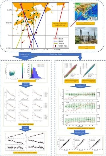
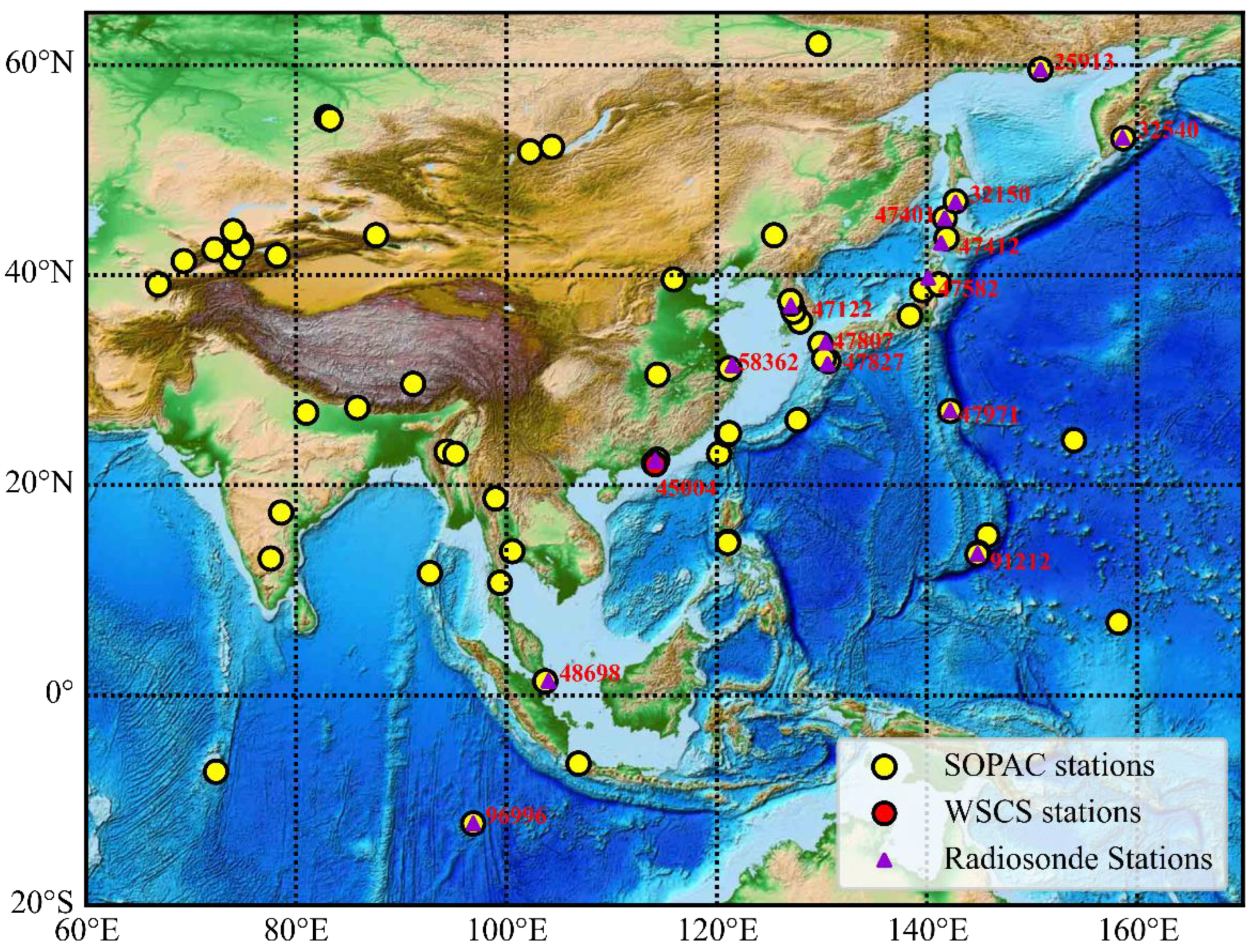
2.1. Dataset

The dataset in this research includes the observation data of PGSs from the WSCS (ftp://1.203.103.214, accessed on 28 July 2022), GNSS Research Center, Wuhan University (GRC, ftp://igs.gnsswhu.cn, accessed on 3 July 2022, Figure 1 and Figure 2), and Hong Kong Geodetic Survey Services (HKGSS, ftp://ftp.geodetic.gov.hk/, accessed on 3 July 2022, Figure 3), as well as the altimeter data of Jason-3 (ftp://ftp-access.aviso.altimetry.fr, accessed on 8 July 2022), HY-2B and HY-2C (https://osdds.nsoas.org.cn/, accessed on 8 July 2022), and radiosonde data from the Department of Atmospheric Science, University of Wyoming (http://weather.uwyo.edu/upperair/sounding.html, accessed on 14 July 2022, Figure 1).

Four PGSs are installed in the WSCS (red dots in Figure 2), and the distances between the four PGSs are less than 30 km, which provides redundant observation data [7]. They are equipped with a STHCR3-G3 Choke Ring antenna and SOUTH Net-S9 receiver. According to the phase center variation tables (http://www.ngs.noaa.gov/ANTCAL/, accessed on 28 July 2022), the antenna phase center stability is within 2 mm. In this research, the PGSs placed on the Zhiwan (ZWAN) and Wailingding (WLDD) islands are used for collection from 24 August 2019 to 30 June 2022 (labeled in Figure 2). The PGS of HKWS has been located approximately 50 km from the WSCS since 2014. This allows for comparisons of their characteristics. The altimeters of Jason-3, HY-2B, and HY-2C fly over this site (Figure 3).

2.2. Processing of GNSS Data

We have two purposes in this research. The first is to define an accurate datum and trend velocities for ZWAN and WLDD PGSs of WSCS. This is achieved through a regional solution together with 61 PGSs which are distributed nearby (Figure 1). The second is to validate the ZWD of the Jason-3, HY-2B, and HY-2C altimeters using the PGSs. The ZWD derived from the PGSs has two methods: (1) the regional solution of the first purpose, and (2) a sub-regional solution with 19 CORS stations of HKGSS (Figure 3).

2.2.1. Processing Methods

The gfzrnx-RINEX toolbox was used for PGS data translation from Rinex 3.04 to 2.11 and data splitting from 1 s to 30 s in this research [25], which was the same method that we used for the data achieved from GRC. Then, the quality of all the PGSs data was checked using the TEQC software developed by the University Nav star Consortium (UNAVCO) facility in Boulder, Colorado [26]. The quality of the PGSs is influenced by the signals reflected by surrounding objects such as water, buildings, trees, etc., which changes the propagation direction, amplitude, polarization, and phase of the signal. These changed signals arrive at the receiver and are superimposed with the signals arriving at the receiver through a straight path. This phenomenon is called multipath effect (MP1 and MP2). The elevation cut-off was set to 10° to eliminate the influence of the multipath signals. The daily data were deleted when the MP1 and MP2 were more than 0.5 m and the time length of the observation was less than 4 h.

The GAMIT/GLOBK (version 10.71) software was used to process the PGS data after the quality check. This software is jointly developed by the Massachusetts Institute of Technology and Scripps Institute of Oceanography [10]. It consists of GAMIT and GLOBK. Using double differencing techniques, the GAMIT component can estimate station positions, satellite orbits, earth orientation parameters, and atmospheric delays from ionosphere-free linear combination GNSS carrier phase observables to eliminate phase biases caused by drifts in the receiver clock and satellite oscillators [10]. The International Earth Rotation Service 2010 (IERS2010) solid Earth tide model, the FES2014 ocean tide model, and the pole tide model were used for data processing [27]. The PGS data in the WSCS were processed using the International GNSS Service (IGS) precise orbits, combined with 61 GNSS stations that are distributed nearby, and collected from the GRC (Figure 1). The total number of GNSS data was 44694 (Figure 2). Following the GAMIT solution, the Kalman filtering techniques were used in GLOBK to estimate the time series, velocities, station positions, and transient deformation [27]. The N, E, and U daily position time series were also provided.

2.2.2. Accuracy Assessment

The normalized root mean square (NRMS) and the weighted root mean square (WRMS) of the daily station position repeatability are objective approaches to assess the quality of GNSS position time series. They were used for the accuracy assessment in the GAMIT/GLOBK solutions. The NRMS would be close to unity with a value of approximately 0.2, if the data are randomly distributed and a priori weights are correct. In this research, the NRMS values of the daily solutions are 0.159~0.199. This means that there were no cycle slips or serious modeling problems [10].

The WRMS measures the noise level of the baseline solution and can be divided into short- and long-term types based on the baseline length of the observation time span [10]. The long-term WRMS reflects the degree of environmental influences, such as nontectonic movement of the monument, atmospheric seasonal changes, orbital long-period error, etc. The WRMS is given as [8]:

$$WRMS=\sqrt{\frac{\frac{\mathrm{n}}{\left(n-2\right)}{\sum }_{i=1}^n\frac{{\left(L_i-L_i^m\right)}^2}{{\sigma }_i^2}}{{\sum }_{i=1}^n{\sigma }_i^2}}$$

(1)

where $L_i$ is the baseline daily solution, ${\sigma }_i$ is the standard deviation for daily solution, $L_i^m$ is the optimal linear fitting value, and n is the number of $L_i$.

2.2.3. Noise Characteristics and Station Velocities

The reformulated maximum likelihood estimation (MLE) in the Hector software was employed to estimate the time series noise characteristics and the station velocities of the PGSs in WSCS [12]. The MLE was given in Equation (2):

$$lik\left(\widehat{v}, C\right)=\frac{1}{\left(2\pi \right)\frac{N}{2}{\left(detC\right)}^{1/2}}\exp \left(-0.5{\widehat{v}}^T{C}^{-1}\widehat{v}\right)$$

(2)

where C is the covariance matrix of assume noise, $\widehat{v}$ is the time series residuals vector between the functional model and the dataset, N is the actual number of observations, and det is the determinant of a matrix.

Hector operates faster than other similar programs, as it accepts only stationary noise for matrix operations [12]. Based on the interquartile range (IQR) of the residuals from the least squares linear fit, the Hector software also allows for the possibility of removing outliers from a time series. The IQR-Factor 2.2 was used to obtain the solutions of the N, E, and U directions of GAMIT/GLOBK. The following relation is used in this research [28]:

sigma = IQR/1.349

(3)

To estimate realistic uncertainties, the power spectral density (PSD) plots and different noise models were used to analyze the time-correlated noise properties. The PSD is usually normalized according to the frequency resolution [29]. It was used in this research to study random vibration signals. Six noise models were applied for analysis using Hector:

• Generalized Gauss–Markov noise (GGM);
• White noise + generalized Gauss–Markov noise (WN + GGM);
• Flicker noise + white noise (WN + FN);
• Random walk + flicker noise (RW + FN);
• White noise + random walk (WN + RW);
• White noise + Power law noise (WN + PL).

The noise in the GNSS time series is temporally correlated. The PSD of the noise can be described by a power-law noise model [30,31]:

$$P\left(f\right)=P_0{\left(\frac{f}{f_0}\right)}^k$$

(4)

where P₀ and f₀ are two constants representing the amplitude and reference frequency, respectively, f is the frequency, and κ is called the spectral index. The Hector software can use the Akaike Information Criteria (AIC) and the Bayesian Information Criteria (BIC) numerical analysis methods based on MLE. These two criteria were used to evaluate the quality of the noise model or the goodness of a chosen noise model and defined in Equations (5) and (6).

$$\mathrm{AIC}=2\mathrm{k}+2\ln \left(lik\right)$$

(5)

$$\mathrm{BIC}=\mathrm{kln}\left(\mathrm{N}\right)+2\ln \left(lik\right)$$

(6)

where the lik is the MLE defined in Equation (2), N is the actual number of observations, and k is the sum of parameters in the matrix H.

Finally, the station velocities of each direction were estimated from the position of PGSs’ daily estimates in ITRF2014. The simplest geometric model for the time series of the N, E, and U directions is a linear trend. The more common expression for the model can be written as follows, including the addition of seasonal term in the brackets in Equation (7) [15]:

$$\begin{array}{c}y\left(t_i\right)=a+b{t}_i+[csin\left(2\pi t_i\right)+dcos\left(2\pi t_i\right)+esin\left(4\pi t_i\right)+fcos\left(4\pi t_i\right)\\ +{\displaystyle \sum _{j=1}^{n_g}}{g}_{j}H\left(t_i+T_{gj}\right)]+v_i\end{array}$$

(7)

where y(t_i) is the position at epoch t (in years), a is the initial position, b is the linear velocity, and c, d, and e, f are the harmonic components of annual amplitudes and the semiannual amplitudes of the sine and cosine functions, respectively. H is the Heaviside step function, n_g is the total number of offsets, g_j is the magnitude of jumps at time T_gj, and v_i signifies the measurement error and denotes noise.

2.3. Validation of the Altimeter ZWD

2.3.1. ZWD from GNSS and Radiosonde

There are many ways to estimate the ZWD, such as radiosonde observations, GNSS, ground-based microwave radiometers, etc. [32,33,34,35]. The intermediate process of GAMIT solutions can be used for research on atmospheric water vapor content, ZWD detection, and weather forecasting. The priori troposphere model used the Vienna Mapping Function (VMF1) to calculate the ZDD and ZWD. The ZWD from the permanent GNSS stations is derived every 0.5 h using the Saastamoinen model in the GAMIT solutions (see Equation (8)) [10,33]:

$$mf\left(E, a, b, c\right)=\frac{(1+\left(a/\left(1+\left(b/\left(1+c\right)\right)\right)\right)}{sinE+a/\left(sinE+b/\left(sinE+c\right)\right)}$$

(8)

where E is the elevation angle (10°); a, b, and c are small (<<1) constants; mf is the TPD. Different sets of coefficients (a_h, b_h, and c_h and a_w, b_w, and c_w) are required for the dry and wet components of TPD (see Equation (9)), respectively.

$$\mathrm{TPD}=mf\left(E,a_h,b_h,c_h\right)\ast \mathrm{ZDD}+mf\left(E,a_w,b_w,c_w\right)\ast \mathrm{ZWD}$$

(9)

The TPD includes the ZWD and ZDD and can be estimated in the GAMIT control files using entries of the mapping function and its coefficients [10].

The radiosondes are usually launched twice per day, at 00:00 UTC and 12:00 UTC. They can provide meteorological information such as temperature, altitude, wind direction and speed, dewpoint, and pressure from the surface to the maximum height of observation [34]. The radiosonde data also provide the saturation vapor pressure, vapor pressure, temperature gradient, relative humidity, and other atmospheric parameters. The ZWD derived from the radiosonde was used to validate the ZWD accuracy of GNSS measurements and altimeters. The ZWD can be calculated from Equation (10) [22]:

$$ZWD=1.763\ast {10}^{-3}{\int }_0^H\left(P_v/T\right)dz$$

(10)

where H is the maximum height of the observation, P_v is the water vapor density (g/cm³), and T is the temperature (K). To achieve an accurate ZWD, the radiosonde data were deleted when the number of data layers was less than 50 and the maximum height was less than 25,000 m.

2.3.2. Validation of the Altimeter ZWD

The MWR onboard satellite mission is combined with the altimeter. Its main task is to correct the range of the altimeters for the path delay resulting from water vapor in the atmosphere, which plays an important role in the precise sea surface height measurements provided by satellite altimeters [2]. The MWR loaded on the altimeters measures the ZWD at three frequencies for Jason-3 (18.7, 23.8, and 34.0 GHz), and HY-2B and HY-2C (18.7, 23.8, and 37.0 GHz). The primary water vapor sensing frequency is at 23.8 GHz. However, the Cal/Val of the altimeter satellite is always performed at an ocean/lake calibration site. The related equipment is placed near the coast and supported by land/island-based laboratories [35]. In the coastal zone, the footprint of MWR is affected by switching from land to ocean or from ocean to land, which produces a problem of missing or inaccurate data.

To conduct accurate validation of the ZWD of the altimeter, the ZWD, computed with the regional network solutions of the 61 PGSs and sub-regional network solutions of the HKGSS described above, were used to assess the ZWD of the Jason-3, HY-2B, and HY-2C altimeter missions in coastal zones. The bias, Root Mean Square (RMS) and correlation coefficient ($R^2$) are defined in the following Equations and used for the validations:

$$bias=\frac{1}{N}\sum _{i=1}^N\left(X_i-Y_i\right)$$

(11)

$$RMS=\sqrt{\frac{{\sum }_{i=1}^N{(X_i-Y_i)}^2}{N}}$$

(12)

$$R^2=\frac{Cov\left(X,Y\right)}{D\left(X\right)D\left(Y\right)}$$

(13)

where N is the matching number, X and Y are the observations from the PGSs data and the MWR, $Cov\left(X,Y\right)$ is the covariance, and the $D\left(X\right) \mathrm{and} D\left(Y\right)$ are variance.

The temporal resolution was 15 min to provide satisfactory consistency between the measurements of PGSs and MWR. An MWR measurement distance of 4~100 km from the coast was analyzed to detect land contamination and improve the ZWD retrieval.

3. GNSS Processing Results

The PGSs of the ZWAN and WLDD daily solutions in the WSCS were processed with 61 additional stations. The time series of daily solutions spanned from 22 August 2019 to 30 June 2022. Following the criteria described above, the PGS data from the WSCS have a missing data rate of approximately 18.44% (WLDD, 858 days in 1052 days) and 15.40% (ZWAN, 890 days in 1052 days). The low missing data rate makes it feasible to perform reliable analysis in the time- and frequency–domain for the PGSs, and define an accurate datum for altimeter calibration in the WSCS.

3.1. WRMS

The daily position WRMS values for the N, E, and U directions was computed. All of the values have a minimum time length of ~2.9 years. The WRMS values of most stations range from 1 to 6 mm, with average values of 2.32 mm and 2.76 mm in the N and E directions, respectively (Figure 4). The WRMS of the U direction ranges from 2.35 to 15.31 mm, and the average value is 8.44 mm, which is about three times that of the N or E direction. This coincides with the availability of a greater number of regional PGSs with favorable geometric distributions. However, some sites with large WRMS values for the U directions (larger than 15 mm) also exist (doy 153, 283, and 358 in 2021). The large WRMS values in the U direction are mainly attributable to instability of the monuments and poor observation conditions (i.e., multipath effect and poor sky visibility) [36]. We decided not to correct or remove the poor data to evaluate the influence of the offsets. Overall, the WRMS values showed high accuracy of the GAMIT/GLOBK solutions [8].

3.2. Noise Properties

As mentioned in Section 2.2.3, the noise properties of the time series were described using six noise models. These models also provided a more realistic velocity uncertainty for the PGSs. The MLE, AIC, and BIC values were used to determine the relative goodness of the time series and to select the best time series for further analysis [12]. Using IQR-Factor 2.2, approximately 1.02%, 0.81%, and 0.66% of the observing data were removed for the N, E, and U directions, respectively.

Figure 5 presents the PSD plots of the time series residuals of the PGSs. The comparison of the plots shows that the time series of the N, E, and U directions tend to follow a linear slope on a logarithmic scale in general [15]. However, more white noise, which was the flat spectrum, seems to appear in the daily solutions. The flatness of the direction noise for the N, E, and U directions was almost the same.

The percentage of the total number of the best noise model based on the three directions is calculated (

Table 1. Statistics of each noise model which has the lowest MLE, AIC, and BIC information criterion values for the N, E, and U directions.

Noise Model	N (%)			E (%)			U (%)			Total (%)
	MLE	AIC	BIC	MLE	AIC	BIC	MLE	AIC	BIC	MLE	AIC	BIC
GGM	4.67	13.33	19.33	4.67	13.33	19.33	4.67	13.33	19.33	4.67	13.33	19.33
WN + GGM	64.00	48.00	43.33	64.00	48.00	43.33	64.00	48.00	43.33	64.00	48.00	43.33
WN + PL	0	6.67	0.67	0	6.67	0.67	0	6.67	0.67	0	6.67	0.67
WN + RW	0	0.67	2.67	0	0.67	2.67	0	0.67	2.67	0	0.67	2.67
FN + RW	0	0.67	2.67	0	0.67	2.67	0	0.67	2.67	0	0.67	2.67
WN + FN	31.33	30.67	31.33	31.33	30.67	31.33	31.33	30.67	31.33	31.33	30.67	31.33

). The largest proportion of the optimal noise model in the total direction is WN + GGM, accounting for 43.33%~68.67% of all sites, followed by WN + FN and GGM. The proportion of the optimal noise model in the three directions is basically the same, indicating that the MLE, AIC, and BIC criteria to select the noise model are reliable [37,38]. However, the AIC and BIC are a bit different from the MLE. Thus, the complex noise in the PGSs coordinate time series underlines the difficulty in applying only one model to all PGSs time series [39].

The PSD plots of the residual time series for WLDD and ZWAN in WSCS and HKWS are presented in Figure 6. Detailed analyses of the noise properties of PGSs are estimated and fitted with theoretical noise models. Accordingly, the best-suited noise models for the three PGSs are WN + GGM for all three directions, followed by WN + FN and GGM. By analyzing the noise types in the N, E, and U directions of a single station, it was found that the directions of most stations show different noise characteristics. In addition, the noise types of stations close to the WSCS stations are not necessarily the same. Therefore, the differences between the directions of PGSs and the space-time differences between stations should be considered when analyzing the noise types of each direction.

3.3. Velocity Estimation

Site velocities/trends and uncertainties were estimated from the time series of daily solutions. The seasonal variations in common mode were accounted as described in Section 2.2.3. The tectonic motion was obtained using the improved time series in the N, E, and U directions. Meanwhile, observations with periods of ~2.9 years are long enough to obtain precise trends/velocities [29]. The velocities derived using the six noise properties were extracted and compared with the data derived from the SOPAC website [37,38]. The “clean trend” (velocity) daily coordinates of the N, E, and U directions for the PGSs of SOPAC were downloaded from ftp://garner.ucsd.edu, accessed on 24 July 2022. We produced the daily time series by removing the mean, coseismic, and nonseismic jumps, as well as the outliers, from the raw trend time series, which was necessary before providing scientific interpretation and the related geophysical processes of GNSS time series.

All velocities and associated uncertainties of the PGSs were compared with the data from SOPAC (Figure 7) using the six noise models. For the U direction, which was very important for the Cal/Val of altimeters, the velocity difference was −1.10~−0.62 mm/year, with uncertainties of 10.17~12.05 mm/year. The velocities and their uncertainties from the GGM noise model compared with SOPAC showed only small differences, and were followed by WN + GGM and WN + PL, with the next-smallest differences. However, the comparisons between the other noise models and SOPAC showed larger differences. This indicates that the other noise models may not be suitable for the analysis. This was different when using MLE, AIC, and BIC criteria. This could be related to the limited length of the time series used in this research. We considered that the most suitable noise models, in this research, were the GGM and WN + GGM models.

The velocities of the WSCS of the six noise models are also shown in

Table 2. PGS velocity of the WSCS. (Unit: mm/year).

PGS	Direction	WN + FN	FN + RW	WN + RW	WN + GGM	GGM	WN + PL
WLDD	N	−10.28 ± 0.69	−10.07 ± 0.92	−9.61 ± 3.38	−10.22 ± 0.42	−10.18 ± 0.35	−10.05 ± 0.61
	E	31.57 ± 0.74	30.98 ± 1.05	30.59 ± 3.39	31.08 ± 0.38	31.10 ± 0.34	31.07 ± 0.42
	U	−3.40 ± 2.10	−2.90 ± 3.42	−5.68 ± 13.57	−2.24 ± 0.69	−2.24 ± 0.63	−2.48 ± 1.79
ZWAN	N	−10.77 ± 0.81	−10.71 ± 1.11	−10.72 ± 4.92	−10.87 ± 0.38	−10.82 ± 0.38	−10.75 ± 0.54
	E	30.93 ± 0.67	30.54 ± 1.07	30.98 ± 4.52	30.69 ± 0.30	30.65 ± 0.30	30.59 ± 0.45
	U	−4.86 ± 2.68	−2.84 ± 3.55	−0.95 ± 19.42	−3.81 ± 0.65	−3.81 ± 0.66	−3.37 ± 1.36
HKWS	N	−10.21 ± 0.75	−10.93 ± 1.09	−10.21 ± 4.80	−11.01 ± 0.34	−10.93 ± 0.36	−10.80 ± 0.58
	E	31.08 ± 0.59	31.16 ± 1.02	31.87 ± 3.94	31.03 ± 0.27	31.02 ± 0.26	31.05 ± 0.37
	U	−2.78 ± 2.11	−1.46 ± 3.51	0.70 ± 14.45	−2.17 ± 0.67	−2.12 ± 0.71	−1.80 ± 1.06

, together with the site of the HKWS, which was approximately 30 km from WLDD. There were no significant differences between the three PGSs on the same plate. This implied that the velocity estimates in this study are reliable and accurate. Combined with the criteria in Section 3.2, the uncertainties of the WN + GGM and GGM noise models were more convenient than those of the other models. Therefore, the mean velocities and uncertainties of the two models were used to estimate the results in this research. They were −10.20 ± 0.39 mm/year, 31.09 ± 0.36 mm/year, and −2.24 ± 0.66 mm/year for the N, E, and U directions for WLDD and −10.85 ± 0.38 mm/year, 30.67 ± 0.30 mm/year, and −3.81 ± 0.66 mm/year for ZWAN, respectively. Time-varying characteristics and nonlinear variations were observed in the ~2.9 years of observations of PGSs in the WSCS (Figure 8).

Although the time length was only ~2.9 years, the N and E directions showed a velocity to the southeast (Figure 8) which was slightly slower than the velocities found by SOPAC for HKWS (−11.50 ± 0.22 mm/year and 32.56 ± 0.19 mm/year). The U direction was downwards, which conflicted with the SOPAC data (0.98 ± 0.61 mm/year). This may be because the SOPAC data were derived from eight years of analysis from 2014 to 2022, while, in this research, only ~2.9 years of data were used. The results of this research will establish a more accurate absolute dynamic datum for the WSCS and provide a more accurate height datum for the calibration of operational altimeters [7].

4. Validation of ZWD

4.1. Comparisons between GNSS Stations and Radiosonde

The accuracy of the ZWD derived from the PGS solutions was validated using the radiosonde data, which was one of the most accurate technologies in the ZWD detection. The relative humidity, pressure, and temperature of the radiosondes with a height of 0~25,000 m were used to calculate the ZWD, as described in Section 2.3.

The coastal radiosonde sites were determined to be less than 50 km from the coastline, with the data downloaded from https://www.ngdc.noaa.gov (accessed on 8 July 2022). Only 18 of the 61 PGS stations mentioned above were used to derive the ZWD values and validate against 14 radiosonde measurements in the regional solution. The temporal–spatial matching criteria were less than 15 min and 50 km [21,23]. The total matching number of data was 18,751. The ZWD bias was noticed for the comparisons ranged −5.02~7.99 mm with an RMS between 14.66 and 27.21 mm (Figure 9).

In the sub-regional solution, there were one radiosonde station (No. 45004) and 19 PGSs in the HKGSS. All the PGSs are within the distance of 50 km from the radiosonde station. The total amount of radiosonde data in the dataset was 41,004 during the research period. The ZWAN and WLDD of WSCS were less than 50 km from the HKGSS, and were processed together in the sub-regional solution. We made comparisons of the ZWD with the PGSs and radiosonde stations with a time span of 15 min (Figure 9). The sub-regional solution was a bit better than the regional solution. However, the results between the ZWAN, WLDD, and HKWS and the radiosonde showed good agreements (

Table 3. Comparisons of ZWD between the radiosonde and PGSs (PGSs—radiosonde). (Unit: mm) The distance was from the radiosonde to the PGSs.

	Station Name	Data Number	Mean	Max	Min	RMS
Regional solution	HKWS	2014	−6.66	48	−61	15.18
	ZWAN	1718	1.29	63.76	−69.03	18.62
	WLDD	1656	−0.54	60.94	−63.38	14.98
Sub-regional solution	HKWS	2014	−7.72	34.83	−58.38	14.53
	ZWAN	1718	1.01	39.64	−56.33	16.59
	WLDD	1656	2.79	40.12	−53.62	15.53

).

Additionally, we compared the ZWD between the PGSs of ZWAN, WLDD, and HKWS in the two solutions (Figure 10). The matching numbers were large and the differences between them were less than 6 mm, and the correlation coefficients were more than 99%. There was no large difference between the regional and sub-regional solutions. Compared with radiosonde, the PGS has the advantage of all-weather capability, low cost, and all-time operation in the ZWD detection. The radiosonde has only two sets of data (12:00 and 0:00), while the PGSs provided 25 data each day. The amount of ZWD of PGSs is much larger than that of radiosonde and the difference between them is smaller. Therefore, the radiosonde was not used in this research for the validation of the altimeter ZWD.

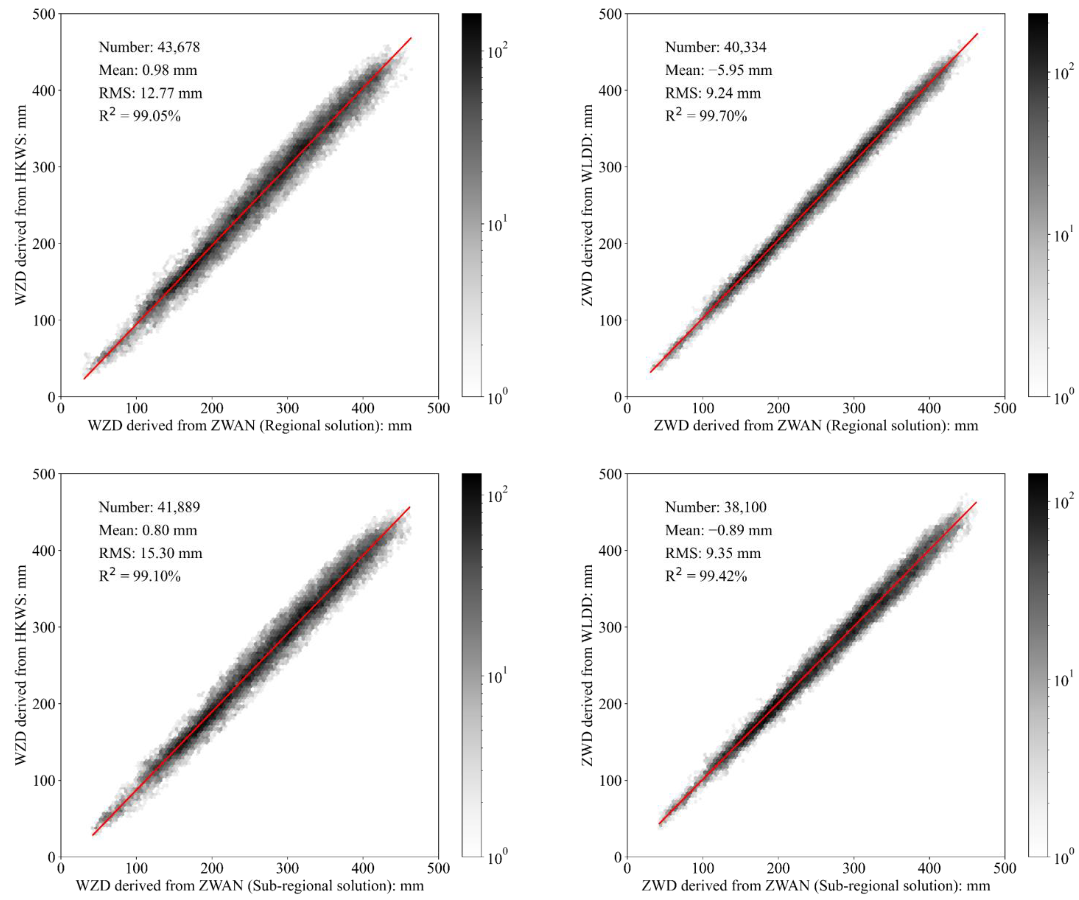
4.2. Validation of the ZWD Using PGSs

These ZWD datasets derived from PGSs were used for the validation of on-board MWR for ZWD corrections of Jason-3, HY-2B, and HY-2C altimeters. This comparison is possible over coastal zones or islands as the PGSs can only be placed on land. A collocated comparison is not possible since there is a spatial overlap of several to dozens of kilometers between terrestrial PGSs and valid measurements from onboard MWRs [32,35]. The comparisons between ZWD derived from PGSs and those from MWRs were analyzed as a function of distance from 4~100 km to the coast with an interval of 2 km in this research. This analysis aims to inspect the land contamination of each MWR to remove this contamination and improve the ZWD retrieval. For each class, the RMS and the number of measurements of these two differences were computed.

Figure 11 shows the comparison results. For Jason-3, the comparison results between PGSs-derived ZWD and the corresponding MWR were −6.2~2.9 mm with an RMS of 10.9~17.9 mm from a distance of 4–30 km. This revealed that the land contamination was less pronounced in MWR. The deviation changed slightly over the distance of 32~100 km. However, the standard deviation gradually increased from 18.8~25.1 mm. For HY-2B, the bias was −1.2~16.2 mm. However, the standard biases were 30.6 mm and more than 30.1 mm when the distances were 14~16 km and more than 28 km, respectively. Therefore, the most suitable distance was 16~28 km, with a bias of 3.8~10.7 mm and a standard bias of 20.9~22.4 mm. For HY-2C, it was obvious that the most suitable distance for matching was 18~30 km. The bias was −8.4~−1.0 mm with a standard bias of 20.2~25.4 mm. Overall, the further the distance between the MWR and PGSs, the greater the difference between the two. The main reason for this was that the spatial variance of the ZWD was large [32,35]. The land contamination was less pronounced for Jason-3 than for HY-2B and HY-2C.

Following the criteria mentioned above, the ZWD values of the Jason-3, HY-2B, and HY-2C altimeters were validated. There were 3476, 1498, and 2919 matching data for Jason-3, HY-2B and HY-2C, respectively, for a time series of ~2.9 years in the regional solution. The comparison dispersion of Jason-3 was lower than those of HY-2B and HY-2C. The validation results were −4.61 ± 16.95 mm, 8.48 ± 23.63 mm, and −5.25 ± 23.48 mm for Jason-3, HY-2B, and HY-2C, respectively. The results showed good agreement between the two measurements, with correlation coefficients of 0.9837, 0.9661, and 0.9641, respectively. The RMS difference may be caused by variability in the MWR at such distances and errors by the mapping function of the GAMIT software. The ZWDs of the Jason-3, HY-2B, and HY-2C altimeters were also validated using the sub-regional solution of WSCS and HKGSS. There were 21 matching PGSs for each of the altimeters. The validation results were −0.21 ± 14.86 mm, 8.81 ± 19.23 mm, and −0.30 ± 17.06 mm for Jason-3, HY-2B, and HY-2C, respectively. These results were a bit better than the regional solution. This may be caused by the smaller scale of the sub-regional solution in the PGSs processing. Validation results of less than 10 mm were shown with correlation coefficients of 0.9841, 0.9691, and 0.9666 for Jason-3, HY-2B, and HY-2C, respectively (Figure 12).

5. Discussion

The PGS time series contain tectonic signals, nontectonic signals, and some unmodeled systematic errors, which are known to affect the estimation of site velocity and its uncertainty. The functional errors can be well explained by deterministic models, whereas the unmodeled errors still remain in the PGS time series. Therefore, a longer time series of analysis is needed. Fortunately, the WSCS is not at the junction of plates. There have been no large earthquakes or strong ruptures around the WSCS since its foundation (http://www.ceic.ac.cn/history, accessed on 15 July 2022), and no sudden jump has occurred in this area.

As an in-situ calibration site for altimeters, the WSCS has been operating since August, 2019 and will keep running for ~2.9 years. It has been used for the on-orbit Cal/Val of HY-2B and HY-2C altimeters and the operational Cal/Val of the HY-2 satellite series. It also has the potential to accomplish the operational Cal/Val for Jason-3, Sentinel-3A, and SARAL/AltiKa altimeters. In previous campaigns, the Jason-3 and Sentinel-3A altimeters has been calibrated and validated using the GNSS and tide gauge in Zhiwan island, which showed good agreements with other in-situ calibration sites [21]. The data, especially on the U direction, were more critical for altimeter calibrations. This will set the precise data for the GNSS buoy or tide gauges in the in-situ measurements of the sea surface height.

6. Conclusions

We presented the processing results of PGSs in and around the WSCS using the regional and sub-regional solutions. Our main concern was, first, to set an accurate datum (especially in U direction) for the altimeter calibration site and, second, to validate the ZWD of the Jason-3, HY-2B, and HY-2C altimeters. We achieved a time series observation of ~2.9 years.

The PGSs of ZWAN and WLDD were processed together with 61 additional stations, achieved from GRC using the GAMIT/GLOBK software in the regional solution. The NRMS and WRMS of the N, E, and U directions showed good results for the solution data. Then, six noise properties of the three directions were analyzed using the Hector software. After comparison of the noise properties, we found that the optimum noise models were WN + GGM and GGM. The station velocities of the PGSs were compared with the SOPAC trend. The results showed that there were no significant differences between them in the N and E directions, and this was a secular motion. However, the velocity of the U direction was contrary to that of SOPAC, which may be caused by the short time periods of the PGS data. The mean velocities and uncertainties were −10.20 ± 0.39 mm/year, 31.09 ± 0.36 mm/year, and −2.24 ± 0.66 mm/year for the N, E, and U directions for WLDD and −10.85 ± 0.38 mm/year, 30.67 ± 0.30 mm/year, and −3.81 ± 0.66 mm/year for ZWAN, respectively.

The ZWD of the PGSs achieved by the GAMIT solution were used to validate the MWRs of Jason-3, HY-2B, and HY-2C in the regional and sub-regional solutions. Before validation, the WZD accuracy of the PGSs was, first, validated using radiosonde data. The differences of −7.72~2.79 mm showed good consistency between the two. To reduce the land contamination of the MWR, a distance of 0~100 km was determined taking 0.5 h GNSS ZWD as a reference value. The ZWD of the PGSs was used to validate the MWRs and the distances of 6~30 km, 16~28 km, and 18~30 km for Jason-3, HY-2B, and HY-2C were determined, respectively. The validation results were −2.30 ± 16.13 mm, 9.22 ± 22.73 mm, and −3.02 ± 22.07 mm for the Jason-3, HY-2B, and HY-2C altimeters, respectively. As the most variable correction of altimeters, the ZWD of Jason-3, HY-2B, and HY-2C was validated in a time series of only ~2.9 years and in the area of interest. The characteristics of longer time series for the bias and RMS of ZTD should be analyzed globally.

References

1. Jiang, X.; Lin, M.; Song, Q. On the Construction of China’s Ocean Satellite Radar Altimetry Calibration Site. Ocean Dev. Manag. 2016, 5, 8–15. [Google Scholar]
2. Quartly, G.D.; Chen, G.; Nencioli, F.; Morrow, R.; Picot, N. An Overview of Requirements, Procedures and Current Advances in the Calibration/Validation of Radar Altimeters. Remote Sens. 2021, 13, 125. [Google Scholar] [CrossRef]
3. Bonnefond, P.; Exertier, P.; Laurain, O.; Guinle, T.; Féméniase, P. Corsica: A 20-Yr multi-mission absolute altimeter calibration site. Adv. Space Res. 2021, 68, 1171–1186. [Google Scholar] [CrossRef]
4. Haines, B.; Desai, S.; Kubitschek, D.; Leben, R. A brief history of the Harvest experiment: 1989–2019. Adv. Space Res. 2021, 68, 1161–1170. [Google Scholar] [CrossRef]
5. Mertikas, S.; Tripolitsiotis, A.; Donlon, C.; Mavrocordatos, C.; Féménias, P.; Borde, F.; Frantzis, X.; Kokolakis, C.; Guinle, T.; Vergos, G.; et al. The ESA Permanent Facility for altimetry calibration: Monitoring performance of radar altimeters for Sentinel3A, Sentinel-3B and Jason-3 using transponder and sea-surface calibrations with FRM standards. Remote Sens. 2020, 12, 2642. [Google Scholar] [CrossRef]
6. Watson, C. Satellite Altimeter Calibration and Validation Using GPS Buoy Technology. Ph.D. Thesis, University of Tasmania, Hobart, Australia, July 2005. [Google Scholar]
7. Chen, C.; Zhu, J.; Ma, C.; Lin, M.; Yan, L.; Huang, X.; Zhai, W.; Mu, B.; Jia, Y. Preliminary Calibration Results of the HY-2B Altimeter’s SSH at China’s Wanshan Calibration Site. Acta Oceanol. Sin. 2021, 40, 129–140. [Google Scholar] [CrossRef]
8. Li, Y. Analysis of GAMIT/GLOBK in high-precision GNSS data processing for crustal deformation. Earthq. Res. Adv. 2021, 1, 100028. [Google Scholar] [CrossRef]
9. Herring, T. MATLAB Tools for viewing GPS velocities and time-series. GPS Solut. 2003, 7, 194–199. [Google Scholar] [CrossRef]
10. Herring, T.; King, R.; McClusky, S. Introduction to GAMIT/GLOBK (Release 10.7); Massachusetts Institute of Technology: Cambridge, MA, USA; Available online: http://geoweb.mit.edu/gg/Intro_GG.pdf (accessed on 22 June 2020).
11. Li, W.; Li, Z.; Jiang, W.; Chen, Q.; Zhu, G.; Wang, J. A New Spatial Filtering Algorithm for Noisy and Missing GNSS Position Time Series Using Weighted Expectation Maximization Principal Component Analysis: A Case Study for Regional GNSS Network in Xinjiang Province. Remote Sens. 2022, 14, 1295. [Google Scholar] [CrossRef]
12. Bos, M.S.; Fernandes, R.M.S.; Williams, S.D.P.; Bastos, L. Fast error analysis of continuous GNSS observations with missing data. J. Geod. 2013, 87, 351–360. [Google Scholar] [CrossRef] [Green Version]
13. Santamaría-Gómez, A.; Bouin, M.-N.; Collilieux, X.; Wöppelmann, G. Correlated errors in GPS position time series: Implications for velocity estimates. J. Geophys. Res. 2011, 116, B01405. [Google Scholar] [CrossRef]
14. Wang, L.; Herring, T. Impact of Estimating Position Offsets on the Uncertainties of GNSS Site Velocity Estimates. J. Geophys. Res. Solid Earth 2019, 124, 13452–13467. [Google Scholar] [CrossRef]
15. Lidberg, M.; Johansson, J.; Scherneck, H.; Davis, J. An improved and extended GPS-derived 3D velocity field of the glacial isostatic adjustment (GIA) in Fennoscandia. J. Geod. 2007, 81, 213–230. [Google Scholar] [CrossRef]
16. Bonafoni, S.; Mazzoni, A.; Cimini, D.; Montopoli, M.; Pierdicca, N.; Basili, P.; Ciotti, P.; Carlesimo, G. Assessment of water vapor retrievals from a GPS receiver network. GPS Solut. 2013, 17, 475–484. [Google Scholar] [CrossRef]
17. Haase, J.; Ge, M.; Vedel, H.; Calais, E. Accuracy and variability of GPS tropospheric delay measurements of water vapor in the western Mediterranean. J. Appl. Meteorol. 2003, 42, 154768. [Google Scholar] [CrossRef]
18. Ablain, M.; Meyssignac, B.; Zawadzki, L.; Jugier, R.; Ribes, A.; Spada, G.; Benveniste, J.; Cazenave, A.; Picot, N. Uncertainty in satellite estimates of global mean sea-level changes, trend and acceleration. Earth Syst. Sci. Data 2019, 11, 1189–1202. [Google Scholar] [CrossRef] [Green Version]
19. Pearson, C.; Moore, P.; Edwards, S. GNSS Assessment of Sentinel-3A ECMWF Tropospheric Delays over Inland Waters. Adv. Space Res. 2020, 66, 2827–2843. [Google Scholar] [CrossRef]
20. Zhang, Y.; Cai, C.; Chen, B.; Dai, W. Consistency evaluation of precipitable water vapor derived from ERA5, ERA-Interim, GNSS, and radiosondes over China. Radio Sci. 2019, 54, 561–571. [Google Scholar] [CrossRef]
21. Zhai, W.; Zhu, J.; Fan, X.; Yan, L.; Chen, C.; Tian, Z. Preliminary calibration results for Jason-3 and Sentinel-3 altimeters in the Wanshan Islands. J. Ocean. Limnol. 2021, 39, 458–471. [Google Scholar] [CrossRef]
22. Wang, J.; Xu, H.; Yang, L.; Song, Q.; Ma, C. Cross-Calibrations of the HY-2B Altimeter Using Jason-3 Satellite During the Period of April 2019–September 2020. Front. Earth Sci. 2021, 9, 647583. [Google Scholar] [CrossRef]
23. Lazaro, C.; Fernandes, J.; Vieira, T.; Vieira, E. A coastally improved global dataset of wet tropospheric corrections for satellite altimetry. Earth Syst. Sci. Data 2019, 12, 3205–3228. [Google Scholar] [CrossRef]
24. Li, F.; Zhang, Q.; Zhang, S.; Lei, J.; Li, W. Evaluation of spatio-temporal characteristics of different zenith tropospheric delay models in Antarctica. Radio Sci. 2020, 55, 1–16. [Google Scholar] [CrossRef]
25. Nischan, T. GFZRNX—RINEX GNSS Data Conversion and Manipulation Toolbox; Version 2.0-8219; GFZ Data Services: Potsdam, Germany, 2016. [Google Scholar] [CrossRef]
26. Estey, L.; Meertens, C. TEQC: The Multi-Purpose Toolkit for GPS/GLONASS Data. GPS Solut. 1999, 3, 42–49. [Google Scholar] [CrossRef]
27. Herring, T.; Melbourne, T.; Murray, M.; Floyd, M.; Szeliga, W.; King, R.; Phillips, D.; Puskas, C.; Santillan, M.; Wang, L. Plate Boundary Observatory and related networks: GPS data analysis methods and geodetic products. Rev. Geophys. 2016, 54, 759–808. [Google Scholar] [CrossRef]
28. He, X.; Yu, K.; Montillet, J.P.; Xiong, C.; Lu, T.; Zhou, S.; Ma, X.; Cui, H.; Ming, F. GNSS-TS-NRS: An Open-Source MATLAB-Based GNSS Time Series Noise Reduction Software. Remote Sens. 2020, 12, 3532. [Google Scholar] [CrossRef]
29. He, X.; Bos, M.; Montillet, J.; Fernandes, R. Investigation of the noise properties at low frequencies in long GNSS time series. J. Geod. 2019, 93, 1271–1282. [Google Scholar] [CrossRef]
30. Williams, S. The effect of coloured noise on the uncertainties of rates estimated from geodetic time series. J. Geod. 2003, 76, 483–494. [Google Scholar] [CrossRef]
31. Nikolaidis, R.M. Observation of Geodetic and Seismic Deformation with the Global Positioning System. Ph.D. Thesis, University of California, San Diego, CA, USA, 2022. [Google Scholar]
32. Xia, P.; Xia, J.; Ye, S.; Xu, C. A New Method for Estimating Tropospheric Zenith Wet-Component Delay of GNSS Signals from Surface Meteorology Data. Remote Sens. 2020, 12, 3497. [Google Scholar] [CrossRef]
33. Kouba, J. Implementation and testing of the gridded Vienna Mapping Function 1 (VMF1). J. Geod. 2008, 82, 193–205. [Google Scholar] [CrossRef]
34. Boehm, J.; Werl, B.; Schuh, H. Troposphere mapping functions for GPS and very long baseline interferometry from European Centre for Medium-Range Weather Forecasts operational analysis data. J. Geophys. Res. 2006, 111, B02406. [Google Scholar] [CrossRef]
35. Vieira, T.; Fernandes, M.J.; Lázaro, C. Independent Assessment of On-Board Microwave Radiometer Measurements in Coastal Zones Using Tropospheric Delays From GNSS. IEEE Trans. Geosci. Remote Sens. 2019, 57, 1804–1816. [Google Scholar] [CrossRef]
36. Zhao, B.; Huang, Y.; Zhang, C.; Wang, W.; Tan, K.; Du, R. Crustal deformation on the Chinese mainland during 1998–2014 based on GPS data. Geod. Geodyn. 2015, 6, 7–15. [Google Scholar] [CrossRef] [Green Version]
37. He, Y.; Zhang, S.; Wang, Q.; Liu, Q.; Qu, W.; Hou, X. HECTOR for Analysis of GPS Time Series. In China Satellite Navigation Conference (CSNC) 2018 Proceedings. CSNC 2018; Lecture Notes in Electrical Engineering; Sun, J., Yang, C., Guo, S., Eds.; Springer: Singapore, 2018; Volume 497. [Google Scholar]
38. Li, Y.; Xu, C.; Yi, L.; Fang, R. A data-driven approach for denoising GNSS position time series. J. Geod. 2018, 92, 905–922. [Google Scholar] [CrossRef]
39. He, X.; Montillet, J.; Fernandes, R.; Bos, M.; Yu, K.; Hua, X.; Jiang, W. Review of current GPS methodologies for producing accurate time series and their error sources. J. Geodyn. 2017, 106, 12–29. [Google Scholar] [CrossRef]
Figure 1. Sketch of the dataset in this research. The yellow circles represent the PGS observations from the GRC used for PGS processing. The dark-violet triangles represent the radiosonde stations used for comparisons with the ZWD of GNSS stations. The red numbers represent the ID number of the radiosonde. The red circle represents the permanent GNSS stations of the WSCS, which is close to the radiosonde (ID: 45004).
Remotesensing 14 06235 g001
Figure 2. Gantt chart of the time series of PGS observations.
Remotesensing 14 06235 g002
Figure 3. Sketch of WSCS and the related satellite altimeters orbits. The red dots represent the permanent GNSS stations of WSCS which were placed on the Zhiwan, Wailingding, Miaowan, and Dangan islands. There is also a PGS installed in Hong Kong (HKWS) from GRC. A total of 19 CORS stations of HKGSS (dark green points) were processed together with the WSCS data to validate the ZWD of the altimeters.
Remotesensing 14 06235 g003
Figure 4. WRMS distributions for the time series of PGSs in the N, E, and U directions. (a) WRMS values for the U direction represented by gradient viridis colors. (b) WRMS distribution for N (green bars), E (red bars), and U (blue bars) directions.
Remotesensing 14 06235 g004
Figure 5. PSD of the N, E, and U directions of the PGSs during the research periods. An observation ratio of less than 70% is not shown.
Remotesensing 14 06235 g005
Figure 6. PSD of the time series residuals of WLDD (top), ZWAN (middle), and HKWS (bottom).
Remotesensing 14 06235 g006
Figure 7. Velocity (left) and uncertainty (right) differences (mm/year) between six selected noise models and SOPAC. The red dots represent the median value between the solution of this research and the SOPAC. The blue lines represent the RMS of the values. The violin is the interquartile range.
Remotesensing 14 06235 g007
Figure 8. Trend of the WLDD (left) and ZWAN (right) PGSs in the N, E, and U directions. The red curves represent the change of each direction after geometric modelling.
Remotesensing 14 06235 g008
Figure 9. The ZWD comparison between the PGSs and radiosonde. Left figure is the comparison between the radiosonde and regional solutions of WSCS. The legend represents the name of the PGSs (four characters) and the ID number of radiosonde (5 digits). The right figure is the comparison between the radiosonde number of 45,004 and the PGSs of HKGSS. The legend represents the name of the PGSs.
Remotesensing 14 06235 g009
Figure 10. Comparisons of regional (top) and sub-regional (bottom) ZWD derived from different PGSs in the WSCS, including ZWAN, WLDD, and HKWS.
Remotesensing 14 06235 g010
Figure 11. Comparison of ZWD derived from PGSs and MWR (MWR—PGSs). The x-axis is the distance between the PGSs and altimeter footprints. The green dots and lines represent the bias and RMS, respectively. The red line represents the matching data number. The HY-2C had no ZWD data when the distance was less than 4 km to the coast.
Remotesensing 14 06235 g011
Figure 12. Validation results of the ZWD of altimeters. The Bias was MWR minus the PGSs.
Remotesensing 14 06235 g012