Article

Application of the Fourier Series Expansion Method for the Inversion of Gravity Gradients using Gravity Anomalies

1
Department of Navigation, Naval University of Engineering, Wuhan 430033, China
2
School of Geography and Information Engineering, China University of Geosciences, Wuhan 430033, China
3
Key Laboratory of Geological Exploration and Evaluation Ministry of Education, China University of Geosciences, Wuhan 430033, China
4
Guangxi Key Laboratory of Spatial Information and Geomatics, Guilin 530001, China
*
Author to whom correspondence should be addressed.
Remote Sens. 2023, 15(1), 230; https://doi.org/10.3390/rs15010230
Submission received: 5 November 2022 / Revised: 22 November 2022 / Accepted: 28 December 2022 / Published: 31 December 2022
(This article belongs to the Section Satellite Missions for Earth and Planetary Exploration)

Abstract

:
Accurate and highly precise gravity gradient data are an important component of, for example, gravity field modeling, seabed topography inversion, and resource exploration. However, high-precision gravity gradient data are difficult to obtain. To address this difficulty, this work introduces the Fourier series expansion method to the modeling of gravity gradient fields. Based on gravity anomalies, the analytic expressions of the gravity gradient tensors have been deduced, which provides a new mathematical method for obtaining gravity gradient data. The expression’s derivation and verification processes are as follows. First, these analytic expressions for inverting the gravity gradient based on gravity anomaly data are derived according to the Laplace equation, the boundary value conditions of spherical approximation, and the Fourier series expansion method. Then, global 1’ × 1’ gravity field data provided by UCSD are used to verify the accuracy of these formulas. Finally, the results are analyzed. The experimental results show that the results obtained based on this inversion formula can sufficiently show the details of gravity gradient changes. The formulas derived in this paper have good computational efficiency in the inversion of regional gravity gradients and provide a new mathematical method for gravity gradient data acquisition.

1. Introduction

As an important physical feature of the earth, measurements of the gravity field have been used in many fields and research projects, such as studies of the Earth’s internal structure, mineral resource exploration, and improving satellite-based navigation [1,2,3,4,5]. The gravity gradient, as the second derivative of the gravity field, offers a greater resolving power than can be obtained from direct gravity measurements. The measurement process is not affected by carrier acceleration, which increases the application potential of the gravity gradient [6,7,8,9].
Since the Hungarian geophysicist Eötvös developed the first gravity gradiometer in 1886, after more than a century of development, gravity gradiometers have been used for engineering applications with very good results [10,11,12,13,14]. The development of gravity gradiometers in China started at the beginning of this century and is still in the stage of testing and verification. However, no domestically produced gravity gradiometers that can be used in engineering applications have been developed yet [15,16]. An effective data verification basis for the development of gravity gradiometers involves establishing a high-precision gravity gradient field. Therefore, it is of critical importance to study the forward and inverse methods of determining gravity gradients, as these methods are the basis of a variety of studies based on gravity gradients.
At present, the theoretical method of gravity gradient forward modeling is very precise. Forsberg deduced the theoretical formula of gravity gradient forward calculation [17]. Since then, different scholars have proposed different numerical calculation formulas based on different discrete model elements [18,19,20,21,22,23,24,25]. Gravity gradient inversion methods are mainly established in the space and frequency domains. In terms of the frequency domain, fast Fourier transform (FFT) is the most common calculation method. In the 1970s, Gunn was the first to use the FFT method for the calculation of gravity fields. Domestic and international scholars have conducted in-depth research on gravity field inversion using the FFT method and have had positive results [26,27,28,29,30]. In the spatial domain, integral methods such as the prism and spherical techniques are mainly used to divide the anomalous body into multiple independent monomers and integrate the gravity gradient at a certain point. In addition, some scholars have studied how a Fourier series can be applied to gravity fields. Harrison and Dickinson studied the application of a Fourier series to a local gravity field model, though this approach mainly solves problems related to distances within airspaces [31]. Monte H applied a Fourier series to gravity data processing, which efficiently functionalizes the data so as to minimize the computational complexity involved in determining the gravity perturbation vector. Ghobadi-Far et al. deduced the Fourier series expression for the potential function of two-position gravity using spherical coordinates [25,31,32,33,34,35,36]. However, there are no studies on the application of the Fourier series expansion method to gravity gradient inversion based on gravity.
Therefore, the Fourier series expansion method is introduced to the gravity gradient inversion for the first time in this study. The Fourier series method offers fast calculation speeds and high accuracies, and it can produce a continuous model. The Fourier series expansion method can be used for the calculation of both discrete fields and continuous fields. Based on the Fourier series expansion method, this work derives and establishes model formulas for gravity gradient based on gravity anomaly data and uses global 1‘× 1’ gravity field data published by UCSD as experimental data to verify the accuracy and applicability of the inversion models. Furthermore, the results are analyzed, and these results are analyzed and discussed systematically.

2. Fourier Series Representation

In this section, the Fourier series representations of gravity potential, gravity, and gravity gradient are derived based on space rectangular coordinates.

2.1. Fourier Series Representation of Gravity Potential

According to Newton’s law of gravity, and based on the separation of variables, the representation of gravity potential can be represented as follows:
T ( x , y , z ) = X ( x )   Y ( y )   Z ( z )
Taking the second derivative of Equation (1) yields
2 T x 2 = d 2 X d x 2   Y ( y )   Z ( z ) 2 T y 2 = d 2 Y d y 2   X ( x )   Z ( z ) 2 T z 2 = d 2 Z d z 2   X ( x )   Y ( y )
Since the gravitational potential satisfies the Laplace equation ( 2 T = 2 T x 2 + 2 T y 2 + 2 T z 2 = 0 ), Equation (3) can be obtained:
d 2 X d x 2   Y ( y )   Z ( z ) + d 2 Y d y 2   X ( x )   Z ( z ) + d 2 Z d z 2   X ( x )   Y ( y ) = 0
Equation (3) can then be written as
1 X   d 2 X d x 2 + 1 Y   d 2 Y d y 2 + 1 Z   d 2 Z d z 2 = 0
Since x   y , and z are independent variables, the following conditions should be satisfied for the above equation to be true for any x, y, or z:
1 X   d 2 X d x 2 = n 2 ω 1 2 1 Y   d 2 Y d y 2 = m 2 ω 2 2 1 Z   d 2 Z d z 2 = n 2 ω 1 2 + m 2 ω 2 2
According to the theory of ordinary differential equations, Equation (5) can be solved:
X = cos n ω 1 x   o r   sin n ω 1 x Y = cos m ω 2 y   o r   sin m ω 2 y Z = e x p ( ± z   n 2 ω 1 2 + m 2 ω 2 2 )
Multiplying X, Y, and Z yields a specific solution to T ( x , y , z ) :
T n   m ( x , y , z ) = e x p ( ± z   n 2 ω 1 2 + m 2 ω 2 2 )   ( cos n ω 1 x , sin n ω 1 x ) · ( A n m B n m C n m D n m ) · ( cos m ω 2 y sin m ω 2 y )
where ω 1 and ω 2 are the eigenvalues of the x and y directions, respectively.
Equation (7) is meaningful only if n and m are positive integers. It is also known that when e x p ( ± z   n 2 ω 1 2 + m 2 ω 2 2 ) or m = n = 0, Equation (7) does not satisfy the regularity condition; thus, the general solution of T ( x , y , z ) can be shown as follows (Equation (8)):
T ( x , y , z ) = n + m N > 0 M e x p ( ± z   n 2 ω 1 2 + m 2 ω 2 2 ) ( cos n ω 1 x , sin n ω 1 x )   ( A n m B n m C n m D n m ) · ( cos m ω 2 y sin m ω 2 y )
If the region K∈ [−N < x < N, −M < y < M] (Z = 0), then ω 1 and ω 2 can be defined as follows:
ω 1 = π N   ω 2 = π M

2.2. Fourier Series Representation of Gravity

Assume that g(x,y) can be represented as
g ( x , y ) = n + m N > 0 M   ( cos n ω 1 x , sin n ω 1 x )   ( a n m b n m c n m d n m ) · ( cos m ω 2 y sin m ω 2 y )
According to the boundary value conditions, a relationship can be represented between g ( x , y ) and T ( x , y ) as Equation (11):
g z ( x , y ) z = 0 = T z = n + m N > 0 M n 2 ω 1 2 + m 2 ω 2 2 ( cos n ω 1 x , sin n ω 1 x )   ( A n m B n m C n m D n m ) · ( cos m ω 2 y sin m ω 2 y )
It can be expressed as Equation (12) by Equations (10) and (11):
( A n m B n m C n m D n m ) = ( a n m b n m c n m d n m ) / n 2 ω 1 2 + m 2 ω 2 2
Similarly, g x ( x , y ) and g y ( x , y ) can be obtained by
g x ( x , y ) z = 0 = n + m N > 0 M n ω 1 n 2 ω 1 2 + m 2 ω 2 2 ( sin n ω 1 x , cos n ω 1 x )   ( a n m b n m c n m d n m ) · ( cos m ω 2 y sin m ω 2 y )
g y ( x , y ) z = 0 = n + m N > 0 M m ω 2 n 2 ω 1 2 + m 2 ω 2 2   ( cos n ω 1 x , sin n ω 1 x )   ( a n m b n m c n m d n m ) · ( cos m ω 2 y sin m ω 2 y )
Therefore, Equations (11), (13), and (14) are Fourier series expressions of gravity. Therefore, ( a n m b n m c n m d n m ) in these expressions is defined by Equation (15):
( a n m b n m c n m d n m ) = 1 ε n ε m N M N N M M g ( x , y ) ( cos n ω 1 x , sin n ω 1 x ) · ( cos m ω 2 y sin m ω 2 y ) d x d y
ε n and ε m in Equation (15) are defined by Equation (16):
ε n = { 2 , n = 0 1 , n 0 ; ε m = { 2 , m = 0 1 , m 0

2.3. Fourier Series Representation of the Gravity Gradient

The gravity gradient is the second derivative of the gravity potential. Thus, the Fourier series expression of the gravity gradient can be obtained by the derivatives of Equations (11), (13), and (14):
g x x ( x , y ) = n + m N > 0 M n 2 ω 1 2 n 2 ω 1 2 + m 2 ω 2 2   ( cos n ω 1 x , sin n ω 1 x )   ( a n m b n m c n m d n m ) · ( cos m ω 2 y sin m ω 2 y )
g x y ( x , y ) = n + m N > 0 M n ω 1   m ω 2 n 2 ω 1 2 + m 2 ω 2 2     ( sin n ω 1 x , cos n ω 1 x )   ( a n m b n m c n m d n m )   ( sin m ω 2 y cos m ω 2 y )
g x z ( x , y ) = n + m N > 0 M n ω 1 ( sin n ω 1 x , cos n ω 1 x )   ( a n m b n m c n m d n m ) · ( cos m ω 2 y sin m ω 2 y )
g y y ( x , y ) = n + m N > 0 M m 2 ω 2 2   n 2 ω 1 2 + m 2 ω 2 2   ( cos n ω 1 x , sin n ω 1 x )   ( a n m b n m c n m d n m ) · ( cos m ω 2 y sin m ω 2 y )
g y z ( x , y ) = n + m N > 0 M m ω 2   ( cos n ω 1 x , sin n ω 1 x )   ( a n m b n m c n m d n m ) · ( sin m ω 2 y cos m ω 2 y )
g z z ( x , y ) = n + m N > 0 M n 2 ω 1 2 + m 2 ω 2 2   ( cos n ω 1 x , sin n ω 1 x )   ( a n m b n m c n m d n m ) · ( cos m ω 2 y sin m ω 2 y )
These equations are the formulas for the gravity gradient inversed by gravity anomalies based on the Fourier series expansion method. Subscripts n and m in these formulas are the truncation order.

3. Data and Experimental Area

3.1. Experimental Area

In this work, considering the influence of terrain on the gravity gradient, the Qinghai–Tibetan Plateau (26–40°N, 73–105°E), and the North China Plain (32–40°N, 114–121°E) are selected as experimental areas to verify the gravity gradient inversion formulas derived from the Fourier series expansion method. The Qinghai–Tibetan Plateau consists of complex and variable terrain and is densely covered with mountains and rivers. Most of the region is between 3000–5000 m above sea level, and it has an average elevation of more than 4000 m. The North China Plain is low and flat, most of the area is less than 50 m above sea level, and the average elevation of the eastern coast is less than 10 m above sea level. Due to the large topographic differences between the Qinghai–Tibetan Plateau and the North China Plain, the selection of these two regions as experimental areas can effectively verify the applicability and accuracy of the Fourier series forward model. The topographic changes in the North China Plain and Qinghai–Tibetan Plateau are shown in Figure 1.

3.2. Data

The data used in this experiment are from the global 1’ × 1’ ‘gravity field dataset published by UCSD (version v29.1), and the data are arranged in a two-dimensional grid. The variations in gravity anomaly data in the study areas are shown in Table 1 and Figure 2a.
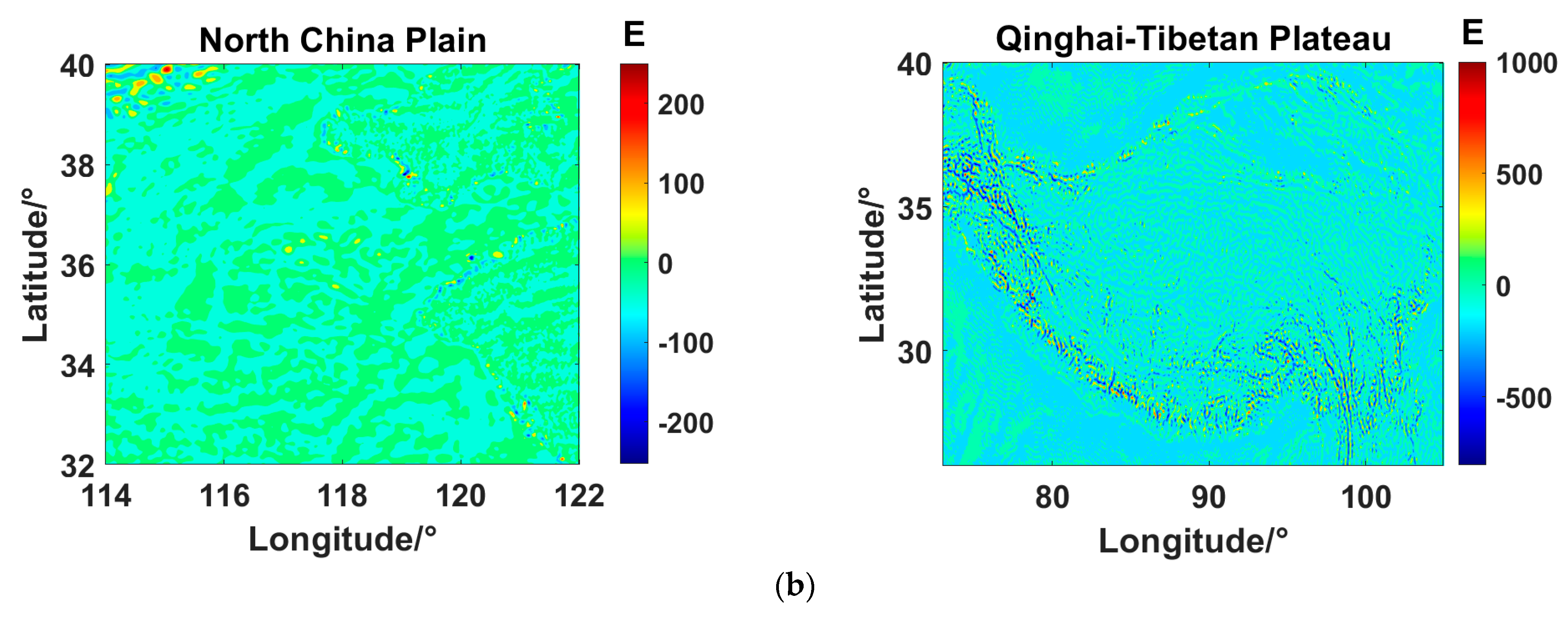
Figure 1 and Figure 2 show that gravity and the gravity gradient are closely related to the terrain. According to the topographic data, the change in gravity and the gravity gradient in the North China Plain and the Qinghai–Tibetan Plateau is consistent with the actual topography. Table 1 and Table 2 show that the gravity gradient has greater changes than the gravity in the same area. The difference between the maximum and minimum gravity gradient is more than 1800 E.
Therefore, the accuracy and applicability of these formulas, as presented in this paper, can be effectively verified using two experimental areas with large topographic differences.

4. Experimental Results and Analysis

For the gravity anomaly data provided by UCSD, the forward model formula derived from the Fourier series expansion method is used to calculate the gravity gradient and analyze the results.

4.1. Experimentation and Analysis

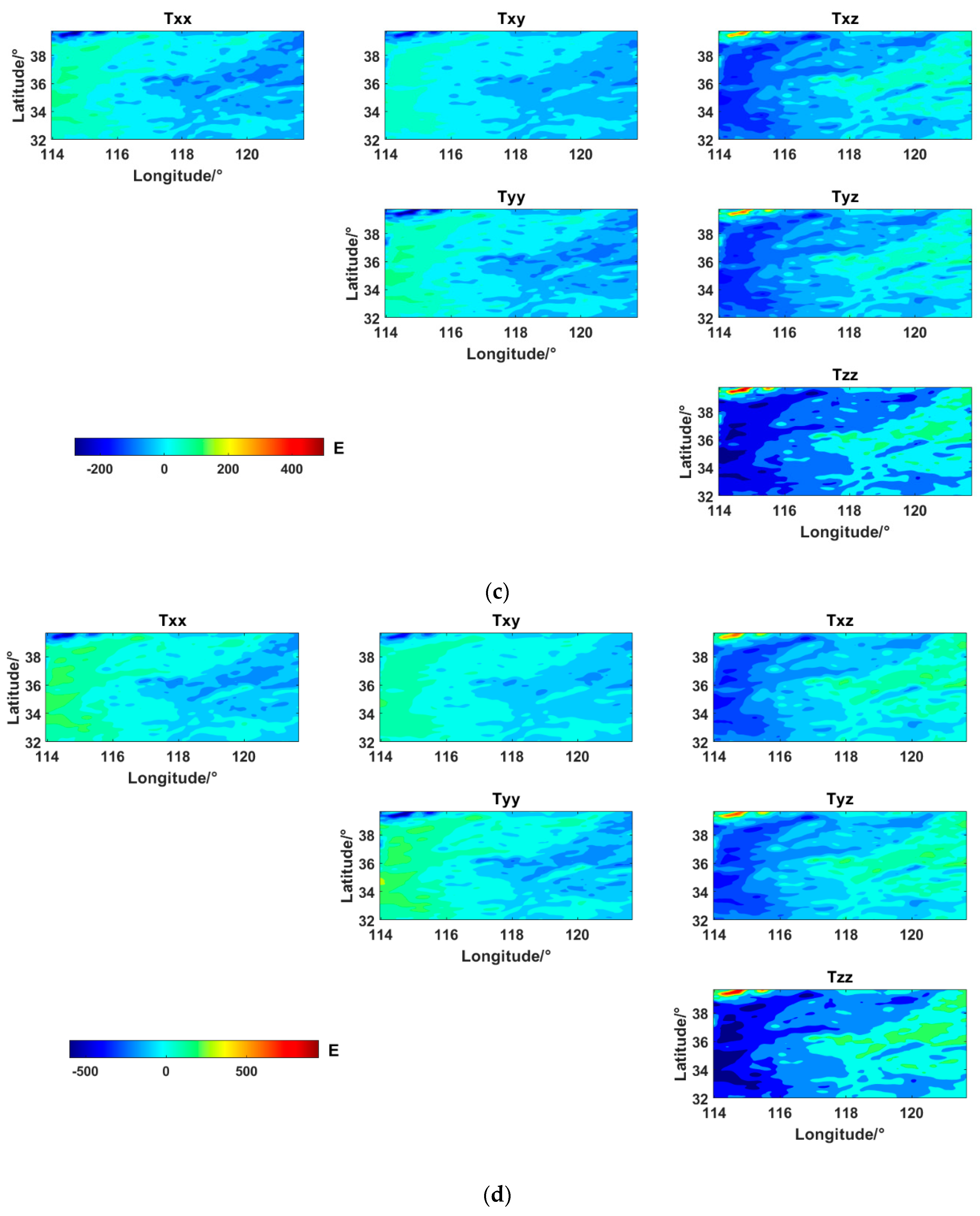
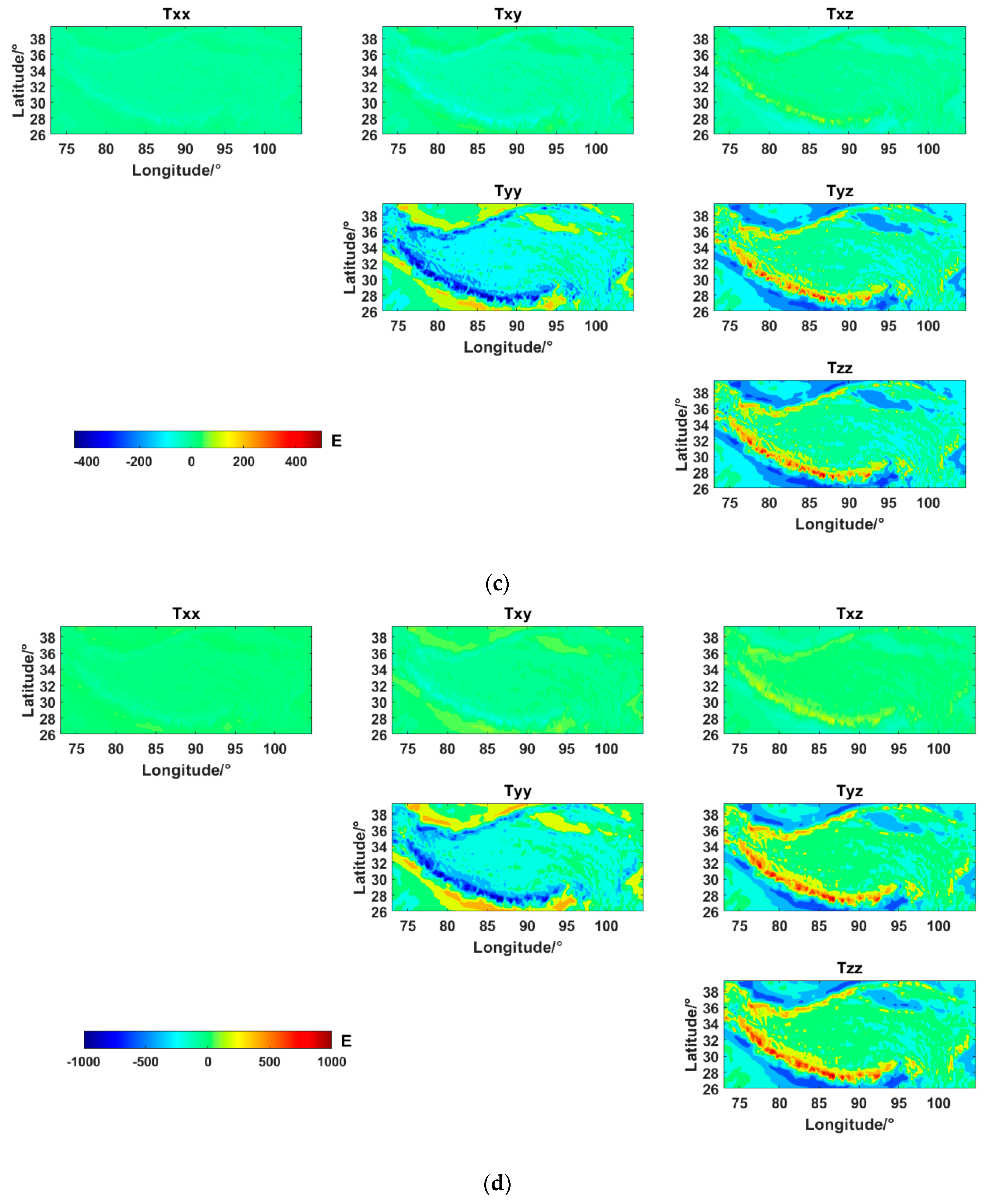
Global gravity anomaly data released by UCSD are used to verify Equations (17)–(22). The precision of the global gravity field data provided by UCSD is better than 1 mGal. The data provided by UCSD can be used to minimize the error increase in the gravity gradient results typically due to inaccurate data sources, which will improve the precision of the results. Based on the experimental data, Fourier series expressions with different truncation orders are calculated for Equations (17)–(22). The experimental results are shown in Figure 3 and Figure 4 and Table 3, Table 4 and Table 5.
Figure 3 and Table 3 show the gravity gradient tensors of the North China Plain based on different truncation orders. According to Figure 3 and Table 3, the minimum of the gravity gradient is in the gxx, and the maximum of the gravity gradient is in the gzz, regardless of the truncation order changes. With the increase in the truncation order, the value of the inversion gravity gradient increases proportionally, and the increased proportion is positively correlated with the increased proportion of the truncation order.
Figure 1 and Figure 3 show that the distribution of the gravity gradient is consistent with topography, and the gravity gradient changes more than the terrain, which contains more geological information.
Figure 4 and Table 4 show the gravity gradient tensors of the Qinghai–Tibetan Plateau based on different truncation orders. According to Figure 4 and Table 4, the minimum of the gravity gradient is in the gyy, and the maximum of the gravity gradient is in the gzz, regardless of the truncation order changes, and the distribution of the gravity gradient is also consistent with the topography of the Qinghai–Tibetan Plateau.
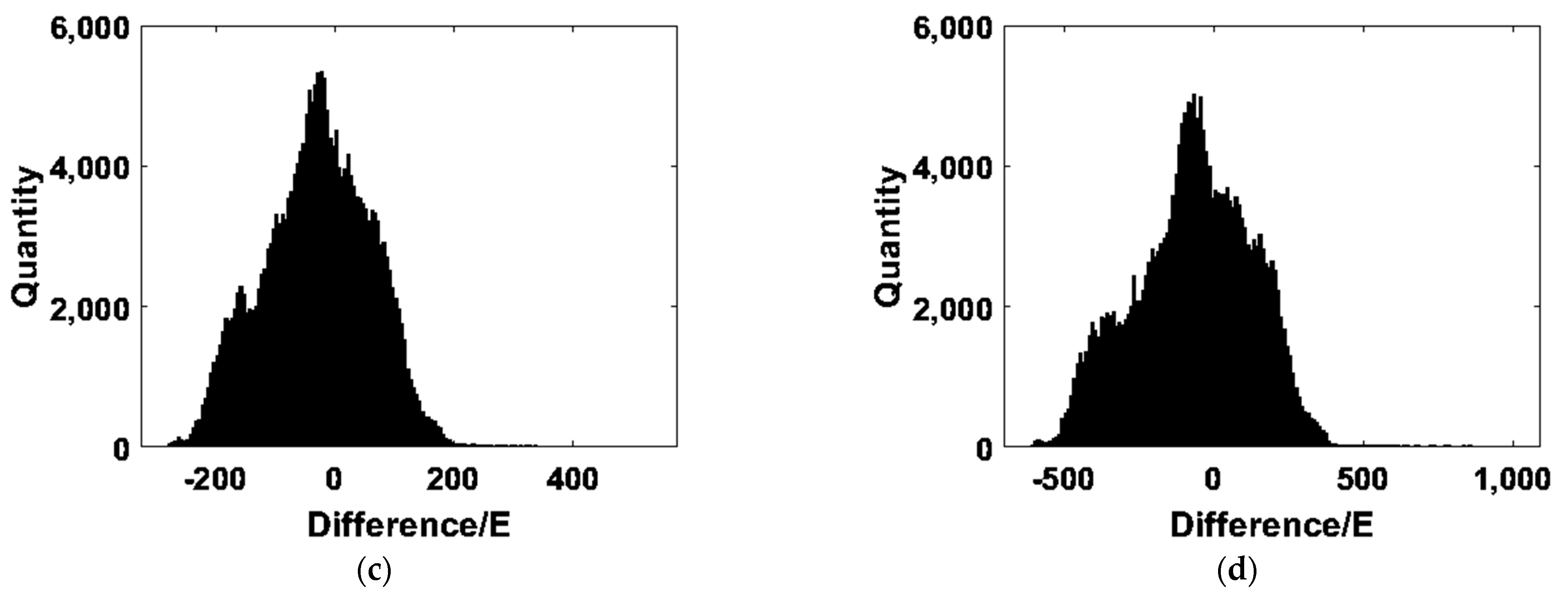
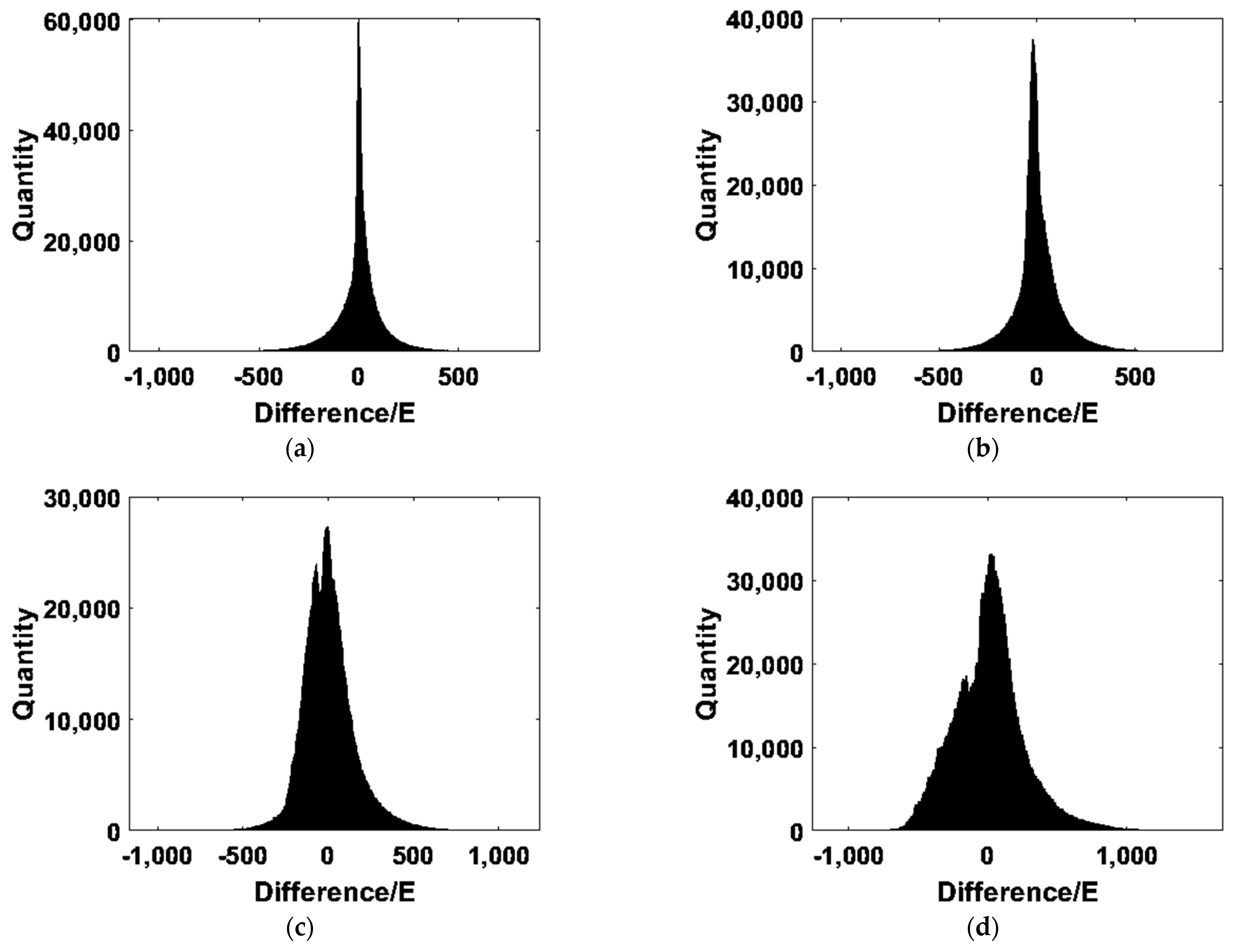
Figure 5 and Figure 6 show the histograms of difference between the vertical gravity gradient calculated by the model and that of the UCSD in the experimental areas. Table 5 shows the difference between the vertical gravity gradient calculated by the model and the gravity gradient provided by UCSD. It can be seen from Figure 5 and Figure 6 that the error is normally distributed, mainly concentrated near zero.
As shown in Figure 3 and Figure 4, increasing the truncation order leads to a decrease in the display ability of the gravity gradient details obtained by inversion. However, it can be seen from Table 3 and Table 4 that, as the truncation order increases, the inversion results will gradually approach the true value, and the inversion result increases. It can be seen from Table 3 and Table 4 that, with the increase in the inversion area, the truncation order also needs to be increased accordingly so that the inversion results converge with the true value.

4.2. The Efficiency of the Calculations

Based on the experimental data, the efficiency of Fourier series expressions with different truncation orders is calculated for Equations (17)–(22) in this section. The statistical results are shown in Table 6.
Table 6 shows that time increases with the increase in the truncation order and the experimental area, and the increase is a multiple of the truncation order and the experimental area. For instance, the multiple of the time increase is approximately equal to the multiple of the truncation order increase in the two experimental areas. The calculation time of the Qinghai–Tibetan Plateau area is about the same as the multiple of that of the North China Plain area, which is equal to the multiple of the data size of the Qinghai Tibet Plateau area compared with that of the North China Plain area.

5. Conclusions

As one of the most important physical characteristics of the Earth, establishing an accurate gravity gradient field is of great importance. This work presented an analytical approach for gravity gradient inversion based on the Fourier series expansion method. The Fourier series offers fast calculation speeds and high accuracies, and it can produce a continuous model. The Fourier series expansion method can be used for the calculation of both discrete fields and continuous fields. Based on the characteristics of a Fourier series, gravity gradient component inversion models were derived as Equations (17)–(22). Then, the global gravity anomaly released by UCSD was used to verify the accuracy and applicability of Equations (17)–(22). The experimental results show that Equations (17)–(22), derived in this paper, are strongly applicable and adaptable in the field of gravity gradient inversion. According to the formulas derived in this paper, the inversion results show the variation details of each component of the gravity gradient. The formulas derived in this paper have good computational efficiency in the inversion of regional gravity gradient.

Author Contributions

Conceptualization, B.L. and S.B.; methodology, B.L.; software, R.Z. and P.X.; validation, R.Z. and P.X.; formal analysis, B.L.; investigation, B.J.; resources, B.J.; writing—original draft preparation, B.L.; writing—review and editing, S.W. and C.C. All authors have read and agreed to the published version of the manuscript.

Funding

This research was funded by the National Natural Science Foundation of China (41874091 and 41971416), the National Science Foundation for Outstanding Young Scholars (No. 42122025), and the National Science Fund for Young Scholars (No. 42104004). The research was also funded by the Guangxi Key Laboratory of Spatial Information and Geomatics (19-185-10-02).

Data Availability Statement

Publicly available datasets were analyzed in this study. These data can be found here: ftp://topex.ucsd.edu/pub/global_grav_1min/ (accessed on 26 July 2022).

Acknowledgments

The gravity data and gravity gradient data were provided by SIO. The authors are indebted to the anonymous reviewers for helping to improve the manuscript.

Conflicts of Interest

The authors declare no conflict of interest. The funders had no role in the design of the study; in the collection, analyses, or interpretation of the data; in the writing of the manuscript; or in the decision to publish the results.

References

  1. Huang, M.; Zhai, G.; Guan, Z. The Determination and Application of Marine Gravity Field; Surveying and Mapping Press: Beijing, China, 2005. [Google Scholar]
  2. Chen, S. The Data Processing, Analysis and Application of Marine Gravity; China Ocean Press: Beijing, China, 1991. [Google Scholar]
  3. Liu, J.; Liu, L.; Liang, X.; Ye, Z. Comparison of methods to model gravity gradient field using gravity anomaly data. Geomat. Inf. Sci. Wuhan Univ. 2015, 40, 1677–1682. [Google Scholar] [CrossRef]
  4. Lu, B.; Barthelmes, F.; Li, M.; Förste, C.; Ince, E.S.; Petrovic, S.; Flechtner, F.; Schwabe, J.; Luo, Z.; Zhong, B.; et al. Shipborne gravimetry in the Baltic sea: Data processing strategies, crucial findings and preliminary geoid determination tests. J. Geod. 2019, 93, 1059–1071. [Google Scholar] [CrossRef]
  5. Xian, P.; Ji, B.; Bian, S.; Liu, B. Influence of sea level anomaly on underwater gravity gradient measurements. Sensors 2022, 22, 5758. [Google Scholar] [CrossRef] [PubMed]
  6. Talukder, A.R.; Bialas, J.; Klaeschen, D.; Buerk, D.; Brueckmann, W.; Reston, T.; Breitzke, M. High-resolution, deep tow, multichannel seismic and sidescan sonar survey of the submarine mounds and associated BSR off Nicaragua pacific margin. Mar. Geol. 2007, 241, 33–43. [Google Scholar] [CrossRef] [Green Version]
  7. Zhang, C.J.; Bian, S.F.; Zhou, X.H.; Fang, J.; Hao, X.G.; Zhang, W.M. Determination of gravity vertical gradient and its application potential. Prog. Geophys. 2007, 22, 1686–1691. [Google Scholar]
  8. Barngrover, C.; Kastner, R.; Belongie, S. Semisynthetic versus real-world sonar training data for the classification of mine-like objects. IEEE J. Ocean. Eng. 2015, 40, 48–56. [Google Scholar] [CrossRef] [Green Version]
  9. Yan, Z.; Ma, J.; Tian, J.; Liu, H.; Yu, J.; Zhang, Y. A gravity gradient differential ratio method for underwater object detection. IEEE Geosci. Remote Sens. Lett. 2014, 11, 833–837. [Google Scholar] [CrossRef]
  10. Gerber, M.A. Gravity gradiometry-something new in inertial navigation. Astronaut. Aeronaut. 1978, 16, 18–26. [Google Scholar]
  11. Chan, H.A.; Moody, M.V.; Paik, H.J. Superconducting gravity gradiometer for sensitive gravity measurements. II. Experiment. Phys. Rev. D 1987, 35, 3572–3597. [Google Scholar] [CrossRef]
  12. Jiang, T.; Hu, C.; Liu, J.; Wu, W. Error analysis of rotating MEMS accelerometer airborne gravity gradiometer under the action of multiple physical fields. J. Huazhong Univ. Sci. Technol. 2022, 50, 83–89. [Google Scholar]
  13. Yu, M. Error Compensation and Signal Processing of a Rotating Accelerometer Gravity Gradiometer; Southeast University: Nanjing, China, 2019. [Google Scholar]
  14. Douch, K.; Panet, I.; Pajot-Métivier, G.; Christophe, B.; Foulon, B.; Lequentrec-Lalancette, M.F.; Diament, M. Error analysis of a new planar electrostatic gravity gradiometer for airborne surveys. J. Geod. 2015, 89, 1217–1231. [Google Scholar] [CrossRef]
  15. Song, H. Precise Measurement of Gravity Gradient Based on the Cold Atom Interferometer; Huazhong University of Science & Technology: Wuhan, China, 2017. [Google Scholar]
  16. Wu, Q.; Teng, Y.T.; Zhang, B.; Zhang, T. The research situation of the gradiometer in the world. Geophys. Geochem. Explor. 2013, 37, 761–768. [Google Scholar]
  17. Forsberg, R. A Study of Terrain Reductions, Density Anomalies and Geophysical Inversion Methods in Gravity Field Modeling; Ohio State Univ Columbus Department of Geodetic Science and Surveying: Columbus, OH, USA, 1984. [Google Scholar]
  18. Jahandari, H.; Farquharson, C.G. Forward modeling of gravity data using finite-volume and finite-element methods on unstructured grids. Geophysics 2013, 78, G69–G80. [Google Scholar] [CrossRef]
  19. Heck, B.; Seitz, K. A comparison of the tesseroid, prism and point-mass approaches for mass reductions in gravity field modelling. J. Geod. 2007, 81, 121–136. [Google Scholar] [CrossRef]
  20. Wild-Pfeiffer, F. A comparison of different mass elements for use in gravity gradiometry. J. Geod. 2008, 82, 637–653. [Google Scholar] [CrossRef]
  21. Li, X.; Chouteau, M. Three-dimensional gravity modeling in all space. Surv. Geophys. 1998, 19, 339–368. [Google Scholar] [CrossRef]
  22. Wang, X. Comparison of Forward Methods of Gravity and Gravity Gradient; China University of Geosciences: Beijing, China, 2018. [Google Scholar]
  23. Bian, S.F. Numerical Solution for Geodetic Boundary Value Problem and the Earth’s Gravity Field Approximation; Wuhan Technical University of Surveying and Mapping: Wuhan, China, 1992. [Google Scholar]
  24. Xiao, S.H.; Bian, S.F. Research on regional model of continuous Fourier series of marine magnetic anomaly field using for the geomagnetic navigation. In Proceedings of the 2nd International Conference on Industrial and Information Systems, IEEE, Dalian, China, 10–11 July 2010; pp. 437–440. [Google Scholar]
  25. Liu, F.M.; Zhang, Y.F.; Jing, X. Gravity gradient Parker’s forward method and application using cosine transform. Acta Geod. Gartogr. Sin. 2013, 42, 177–183. [Google Scholar]
  26. Liu, J.Z.; Liang, X.H.; Ye, Z.R.; Liu, Z.K.; Lang, J.J.; Wang, G.C.; Liu, L.T. Combining multi-source data to construct full tensor of regional airborne gravity gradient disturbance. Chin. J. Geophys. 2020, 63, 3131–3143. [Google Scholar] [CrossRef]
  27. Liu, J.Z. Using gravity gradient component and their combination to interpret the geological structures in the eastern Tianshan mountains. Geophys. J. Int. 2022, 228, 982–998. [Google Scholar] [CrossRef]
  28. Wu, L.; Chen, L.; Wu, B.; Cheng, B.; Lin, Q. Improved Fourier modeling of gravity fields caused by polyhedral bodies: With applications to asteroid Bennu and comet 67P/Churyumov–Gerasimenko. J. Geod. 2019, 93, 1963–1984. [Google Scholar] [CrossRef]
  29. Gunn, P.J. Linear transformations of gravity and magnetic fields. Geophys. Prospect. 1975, 23, 300–312. [Google Scholar] [CrossRef]
  30. Zhao, W.; Sneeuw, N. Discussion on a Fourier expression suited for local gravity field modeling. Sci. Surv. Mapp. 2014, 39, 20–25. [Google Scholar] [CrossRef]
  31. Harrison, J.C.; Dickinson, M. Fourier transform methods in local gravity modeling. Bull. Géod. 1989, 63, 149–166. [Google Scholar] [CrossRef]
  32. Ghobadi-Far, K.; Sharifi, M.A.; Sneeuw, N. 2D Fourier series representation of gravitational functionals in spherical coordinates. J. Geod. 2016, 90, 871–881. [Google Scholar] [CrossRef]
  33. Nagy, D.; Papp, G.; Benedek, J. The gravitational potential and its derivatives for the prism. J. Geod. 2000, 74, 552–560. [Google Scholar] [CrossRef]
  34. Tziavos, I.N.; Sideris, M.G.; Forsberg, R.; Schwarz, K.P. The effect of the terrain on airborne gravity and gradiometry. J. Geophys. Res. Solid Earth 1988, 93, 9173–9186. [Google Scholar] [CrossRef]
  35. Dransfield, M.; Zeng, Y. Airborne gravity gradiometry: Terrain corrections and elevation error. Geophysics 2009, 74, I37–I42. [Google Scholar] [CrossRef]
  36. Wallenstein, M. Manipulation of gravity anomaly data using Fourier series. In Proceedings of the IEEE 1971 Conference on Engineering in the Ocean Environment, San Diego, CA, USA, 21–24 September 1971; pp. 280–285. [Google Scholar] [CrossRef]
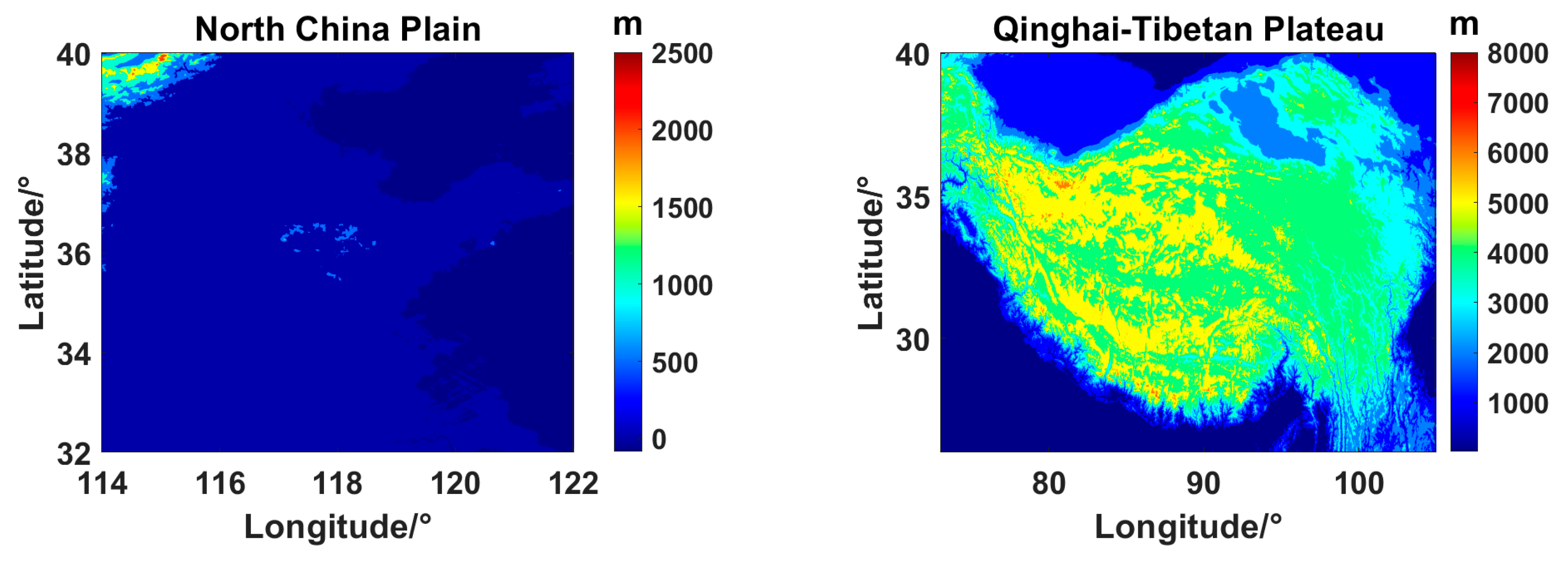
Figure 1. Topography maps.
Remotesensing 15 00230 g001
Figure 2. Gravity field data from the UCSD: (a) gravity; (b) gravity gradient.
Remotesensing 15 00230 g002aRemotesensing 15 00230 g002b
Figure 3. Diagram of inversion results from the North China Plain: (a) 5 × 5 truncation order, (b) 10 × 10 truncation order, (c) 15 × 15 truncation order, (d) 20 × 20 truncation order.
Remotesensing 15 00230 g003aRemotesensing 15 00230 g003b
Figure 4. Diagram of inversion results from the Qinghai–Tibetan Plateau: (a) 5 × 10 truncation order, (b) 10 × 20 truncation order, (c) 15 × 30 truncation order, (d) 20 × 40 truncation order.
Remotesensing 15 00230 g004aRemotesensing 15 00230 g004b
Figure 5. Diagram of the difference between the vertical gravity gradient calculated by the model and that of the UCSD in the North China Plain: (a) 5 × 5 truncation order, (b) 10 × 10 truncation order, (c) 15 × 15 truncation order, (d) 20 × 20 truncation order.
Remotesensing 15 00230 g005aRemotesensing 15 00230 g005b
Figure 6. Diagram of the difference between the vertical gravity gradient calculated by the model and that of the UCSD in Qinghai–Tibetan Plateau: (a) 5 × 10 truncation order, (b) 10 × 20 truncation order, (c) 15 × 30 truncation order, (d) 20 × 40 truncation order.
Remotesensing 15 00230 g006
Table 1. Statistics of the UCSD gravity data. Unit: mGal.
Experimental AreaMinMaxMeanSTD
North China Plain−57.53157.39−4.5416.98
Qinghai-Tibetan Plateau−342.69638.270.5193.53
Table 2. Statistics of the UCSD vertical gravity gradient unit: E (Eötvös).
Experimental AreaMinMaxMeanSTD
North China Plain−252.77276.10−0.5015.18
Qinghai–Tibetan Plateau−806.441070.06−0.06115.95
Table 3. Statistical table of experimental results from the North China Plain. Unit: E (Eötvös).
Truncation OrderGravity GradientMinMaxMeanSTD
5 × 5gxx−20.146.710.642.32
gxy−14.564.820.461.66
gxz−8.7526.11−0.843.02
gyy−18.316.060.582.09
gyz−8.0824.27−0.772.79
gzz−12.7437.36−1.224.39
10 × 10gxx−110.8945.554.4315.25
gxy−82.9433.033.2311.20
gxz−59.60140.69−5.8219.97
gyy−110.8043.754.3114.90
gyz−57.51141.39−5.6619.54
gzz−88.71203.01−8.7429.87
15 × 15gxx−284.16138.0813.9145.77
gxy−210.15102.2110.2834.18
gxz−181.70358.19−18.3760.21
gyy−277.83139.7414.2246.92
gyz−181.97364.88−18.5160.88
gzz−276.28530.98−28.1391.48
20 × 20gxx−528.64299.0630.9197.94
gxy−408.84224.7023.2774.58
gxz−396.98672.29−41.11129.65
gyy−528.64317.0033.24105.04
gyz−409.91710.83−42.85135.07
gzz−615.70995.12−64.15199.89
Table 4. Statistical table of experimental results from the Qinghai–Tibetan Plateau. Unit: E (Eötvös).
Truncation OrderGravity GradientMinMaxMeanSTD
5 × 10gxx−2.751.33−0.010.42
gxy−6.002.96−0.010.94
gxz−3.446.970.011.09
gyy−27.5913.56−0.054.27
gyz−14.0428.520.064.42
gzz−14.7829.860.064.66
10 × 20gxx−16.828.60−0.072.76
gxy−36.5018.81−0.146.22
gxz−21.7242.350.177.17
gyy−174.8089.26−0.6629.95
gyz−91.67180.630.6830.96
gzz−94.72189.160.7332.45
15 × 30gxx−49.3123.89−0.308.43
gxy−110.6252.57−0.6519.10
gxz−60.51125.950.7621.93
gyy−532.21258.01−3.1293.93
gyz−266.92548.633.2497.02
gzz−280.00570.683.42101.47
20 × 40gxx−99.7450.75−0.8818.64
gxy−223.71118.77−1.9742.41
gxz−136.07247.122.2948.59
gyy−1122.91592.25−9.70211.31
gyz−612.011150.6610.05218.10
gzz−640.831182.6910.58227.78
Table 5. The difference between the vertical gravity gradient calculated by the model and that of the UCSD. Unit: E (Eötvös).
Truncation OrderMinMaxMeanSTD
North China Plain5 × 5−275.22244.53−0.7213.85
10 × 10−284.20222.49−8.1929.93
15 × 15−324.73569.58−27.5789.96
20 × 20−606.081033.57−63.54198.27
Qinghai–Tibetan Plateau5 × 10−1058.32814.500.07116.39
10 × 20−1052.27854.470.62120.20
15 × 30−1057.011132.263.21152.25
20 × 40−1127.591553.1010.32253.07
Table 6. The different truncation order times. Unit: s.
Truncation Orders5 × 510 × 1015 × 1520 × 20
North China Plain9.830.161.5103.1
Data size479 × 477
Truncation orders5 × 1010 × 2015 × 3020 × 40
Qinghai–Tibetan Plateau118.3401.8841.51389.5
Data size1917 × 831
Disclaimer/Publisher’s Note: The statements, opinions and data contained in all publications are solely those of the individual author(s) and contributor(s) and not of MDPI and/or the editor(s). MDPI and/or the editor(s) disclaim responsibility for any injury to people or property resulting from any ideas, methods, instructions or products referred to in the content.