Quantifying the Reliability and Uncertainty of Satellite, Reanalysis, and Merged Precipitation Products in Hydrological Simulations over the Topographically Diverse Basin in Southwest China

Abstract

With the continuous emergence of remote sensing technologies and atmospheric models, multi-source precipitation products (MSPs) are increasingly applied in hydrometeorological research, especially in ungauged or data-scarce regions. This study comprehensively evaluates the reliability of MSPs and quantifies the uncertainty of sources in streamflow simulation. Firstly, the performance of seven state-of-the-art MSPs is assessed using rain gauges and the Block-wise use of the TOPMODEL (BTOP) hydrological model under two calibration schemes over Jialing River Basin, China. Then, a variance decomposition approach (Analysis of variance, ANOVA) is employed to quantify the uncertainty contribution of precipitation products, model parameters, and their interaction in streamflow simulation. The MSPs include five satellite-based (GSMaP, IMERG, PERCDR, CHIRPS, CMORPH), one reanalysis (ERA5L), and one ensembled product (PXGB2). The results of precipitation evaluation show that the MSPs have temporal and spatial variability and PXGB2 has the best performance. The hydrologic utility of MSPs is different under different calibration methods. When using gauge-based calibration parameters, the PXGB2-based simulation performs best, whereas CHIRPS, PERCDR, and ERA5L show relatively poor performance. In comparison, the model recalibrated by individual MSPs significantly improves the simulation accuracy of most MSPs, with GSMaP having the best performance. The ANOVA results reveal that the contribution of precipitation products to the streamflow uncertainty is larger than model parameters and their interaction. The impact of interaction suggests that a better simulation attributes to an optimal combination of precipitation products and model parameters rather than solely relying on the best MSPs. These new findings are valuable for improving the suitability of MSPs in hydrologic applications.

1. Introduction

Accurate and reliable precipitation information is desirable for understanding hydrological processes at regional and basin scales [1,2]. Traditionally, precipitation can be monitored through rain gauge networks. However, its regional representation is affected by topography, strong spatial heterogeneity, and the irregular distribution of gauge networks [3,4]. Meanwhile, obtaining adequate or real-time gauge observations is challenging for data confidentiality (e.g., transboundary regions) and technical reasons.

Quickly developing satellite technologies and atmospheric models provide an unprecedented opportunity for hydrological applications of precipitation estimates [5,6]. Multi-source precipitation products (MSPs) such as the Remotely Sensed Information using Artificial Neural Networks (PERSIANN) [7], Integrated MultisatellitE Retrievals for GPM (IMERG) [8], Global Satellite Mapping of Precipitation (GSMaP) [9], Climate Hazards Group InfraRed Precipitation with Station data (CHIRPS) [10], and Global Land Data Assimilation System (GLDAS) precipitation products [11], are extensively used for hydrological simulation and disaster monitoring (e.g., floods, droughts, debris flows) because of their high spatiotemporal resolutions and free availability. Nevertheless, MSPs are subject to various spatial and temporal uncertainties. For instance, satellite-based precipitation products are susceptible to data sources, retrieval algorithms, and sampling frequencies. Reanalysis products are affected by atmospheric conditions and model structure. These biases could be propagated in streamflow simulations, resulting in unreliable guidance for designers and decision-makers. Therefore, it is essential to evaluate the accuracy of MSPs to describe precipitation characteristics [12].

The mainstream approaches to assessing MSPs and their hydrological utilities could be summarized in three ways: (1) Comparing MSPs with gauge observations by using various statistical metrics, which is the most typical and efficient approach. For instance, Lei et al. [13] evaluated six satellite products based on rain gauges and demonstrated that GSMaP and IMERG generally have better performance than others over China. Xu et al. [14] explored the difference between the latest reanalysis products (the latest fifth generation of European ReAnalysis (ERA5) and ERA5-Land) and satellite products (GSMaP and IMERG) using 2200 rain gauges over China. The results showed that satellite products outperform reanalysis products, but the latter perform better than the former in winter and in high latitude areas. Multitudinous similar studies have also been carried out in Bhutan [15], the Adige Basin (Italy) [16], Malaysia [17], South Korea [18], and Canada [19]. These studies reveal a common phenomenon that no single product consistently best represents precipitation distribution across all regions and seasons. (2) Assessing the spatially continuous errors of three or more independent MSPs based on the triple collocation method (TC) without needing “ground truth” [20,21]. It is an essential complement to the gauge-based evaluation approach and is especially suitable for complex areas with inadequate data, such as the accuracy analysis over the Tibetan plateau carried out by Wu et al., Lei et al., and Li et al. [22,23,24]. Wild et al. [25,26] also employed the TC method to evaluate the precipitation error of multiple products over Australia and the Southwest Pacific Region. These results demonstrate that precipitation products have obvious errors in space. (3) Taking multiple MSPs as the forcing data of hydrological models and comparing the impact of precipitation uncertainty on streamflow. In this way, Jiang and Bauer-Gottwein [27] investigated the hydrological utility of IMERG products for 300 basins over China. The results showed that the IMERG Early run is more suitable for flood prediction while the Final run performs better for hydrological modeling in ungauged basins. Su et al. [28] found that TMPA 3B42V7 and IMERG are reliable precipitation sources to guide hydrological modeling in South China, while IMERG slightly outperforms 3B42V7. Tian et al. [29] examined the effects of six precipitation products on monthly hydrological simulation in the Mekong River Basin, discovering that APHRODITE achieved more accurate simulations than other products. From the above-described studies, the gauge-based and TC-based evaluation methods have been applied comprehensively, while the hydrologic assessment approach still has some limitations. The existing studies regarding the hydrological effects of precipitation have mainly focused on a few products (e.g., the same products with different versions, the products from the same sources), failing to consider the latest products such as GSMaP and ERA5-Land, let alone their ensembled products. An up-to-date understanding of the hydrological applications of different latest input sources is needed.

Input uncertainties induced by precipitation may be amplified or reduced by complex and nonlinear hydrological processes [30]. A precipitation product with better performance does not guarante to improve simulated streamflow, which has been reflected and demonstrated in some studies [29,31,32,33]. The uncertainty of streamflow simulation is not only related to precipitation input but also induced by the structure and parameters of hydrological models [34]. Understanding the primary sources of uncertainty is essential for improving model simulation reliability. Many uncertainty quantification frameworks have been introduced to investigate the effects of these uncertainties on streamflow simulation, including the Bayesian uncertainty framework [35,36], the generalized likelihood uncertainty estimation (GLUE), and the Monte Carlo approach [37]. However, most studies have focused on exploring one or two aspects of hydrological modeling uncertainty, which is insufficient to explain why the best precipitation product may not achieve satisfactory simulation results. The interaction between individual sources also contributes to the uncertainty of the simulation, which may be larger than the independent effect and is non-negligible in the total uncertainty [38].

In recent years, the analysis of variance method (ANOVA) [39] has been proposed and has been used in several hydrometeorological studies. It is designed to reveal the respective uncertainty contributions of different sources, especially for their interactions. For example, Mockler et al. [38] assessed the relative importance of parameters, forcing data, and their interactions in hydrological simulation over 31 catchments in Ireland. The Generalised Linear Model was applied to quantify the precipitation forcing rather than input different precipitation products. Qi et al. [31] analyzed the impacts of the six precipitation products, two hydrological models, and their interactions on streamflow uncertainties in the Biliu basin. Ma et al. [40] employed ANOVA to decompose the uncertainties that arise from three precipitation inputs (TRMM 3B42RTv7, 3B42v7, gauge-based) and two hydrological models in the Ganjiang River basin. Besides, Zhou et al. [41] investigated the uncertainties of rain gauges, models, and their interplay by designing nine input gauge levels and three hydrological models. Although some findings about uncertainty source tracing have been revealed in previous studies, to the best of our knowledge, the topic of how and to what extent the state-of-the-art MSPs (including their ensembled product) and their interactions with model parameters affect hydrological processes remains poorly studied.

The principal objectives of this study are: (1) to demonstrate the reliability of seven precipitation products by comparing them with gauge observations in the largest tributary of the Yangtze River; (2) to investigate the hydrological utility of MSPs using the hydrological model through two calibration schemes; (3) to quantify the contribution of MSPs, model parameters, and their interactions to streamflow simulation uncertainty employing the ANOVA method.

2. Data and Methods

2.1. Study Area

The Jialing River (JLR) basin (Figure 1), located in southwest China, is the largest tributary of the Yangtze River basin. It is a vital source of sediment and flood for the Three Gorges Reservoir. The length of the JLR is 1119 km, with an area of 160,000 km². The JLR originates in the Qinling Mountains and flows through Shaanxi, Gansu, Sichuan, and Chongqing provinces. Its elevation decreases significantly from northwest to south, varying from 5211 m to 174 m. The terrain is characterized by mountains in the upstream regions and plains in the lower reaches. The JLR is dominated by a temperate climate. The average annual precipitation and temperature are about 900 mm and 17 °C, respectively. The interannual distribution of precipitation is uneven and mainly concentrated from May to September. Frequent heavy rain in summer is the main contribution to flood disasters in the middle reaches of the Yangtze River. In addition, the streamflow of the JLR is greatly influenced by dams and reservoirs.

2.2. Data

2.2.1. Rain Gauge Precipitation and Streamflow Data

The daily precipitation of 61 rain gauges in the JLR provided by the China Meteorological Administration (CMA) is collected in this study, which has undergone strict quality control and time zone conversion (from Beijing time to UTM time). Most gauges are distributed along the river network (Figure 1), and the average control area of a single gauge is around 2600 km². In addition, the observed daily streamflow of the Beibei hydrological station from 2001 to 2006 is obtained from the Hydrological Bureau of the Ministry of Water Resources in China.

2.2.2. Precipitation Products

Seven precipitation products retrieved by different sources and algorithms are used to investigate their reliability and hydrological utility. The detailed information on precipitation products is presented in

Table 1. The information of precipitation products used in this study.

Products	Resolution	Temporal Span	Reference	Retrieval Algorithm
GSMaP	1 h; 0.1°	2000–present	Kubota et al. [9]	Kalman filtering technique
IMERG	0.5 h; 0.1°	2000–present	Huffman et al. [8]	Goddard profiling algorithm
PERCDR	3 h; 0.25°	1983–2021	Hsu et al. [7]	Adaptive ANN
CHIRPS	daily; 0.05°	1981–present	Funk et al. [10]	‘Smart’ interpolation techniques
CMORPH	3 h; 0.25°	1998–2019	Joyce et al. [42]	Morphing technique
ERA5L	1 h; 0.1°	1950–present	Hersbach et al. [43]	IFS Cy41r2 4D-Var
PXGB2	daily; 0.1°	2000–2017	Lei et al. [44]	XGBoost regression and classification

.

The GSMaP [9] is a high spatial and temporal resolution product developed by the Japan Aerospace Exploration Agency (JAXA) and Japan Science and Technology Agency, which incorporates infrared (IR) satellite observations and passive microwave (PMW) to obtain precipitation estimates. The GSMaP_Gauge product used in this study is a gauge-adjusted product of the GSMaP using Climate Prediction Center (CPC) gauge data analysis. IMERG [8] is the level 3 product of the Global Precipitation Measurement (GPM) algorithm, which is the successor of TMPA. Compared with TMPA, IMERG has made great improvements in capturing rainfall and snowfall, temporal resolution, and spatial coverage. The post real-time “Final run” (IMERG_F) product is chosen in this study. IMERG_F is gauged-adjusted by GPCC monthly rain gauge analysis. PERSIANN-CDR (herein PERCDR) [7] is a long period product covering near forty years (from 1983 to 2021). It incorporates IR information from multi-sensors and gauge data from GPCC but does not include MW signals. The version 2 CHIRPS product [10] has a higher resolution than other products. It combines IR, gauge, and reanalysis information and is suitable for long-term series hydrometeorological research. In addition, the Climate Prediction Center MORPHing technique (CMORPH) [40] bias-corrected (CRT) dataset (herein CMORPH) is employed in this study.

The ERA5-Land (herein ERA5L) product [43] is an enhanced land atmospheric reanalysis product of ERA5. It has higher spatial resolution compared with ERA5 and the older ERA-Interim. The latest ERA5L has been evaluated and proved to have good application potential over China [14]. The PXGB2 product is a multi-source precipitation merged product prepared by Lei et al. [44] based on a two-step merging strategy. This merging strategy employs the extreme gradient boosting (XGBoost) classification and regression models to combine relatively dense gauges, reanalysis, and satellite precipitation data. The spatial coverage of PXGB2 is mainland China (15–56°N, 70–140°N). For more detailed information about PXGB2, refer to Lei et al. [44].

2.2.3. Hydrological Model Input Datasets

In addition to precipitation, input data for the hydrological model mainly include DEM, leaf area vegetation index (LAI), interception loss (PET), potential evapotranspiration (EP), soil, and land use data.

The DEM is downloaded from Shuttle Radar Topography Mission (SRTM) with 30 m spatial resolution. Due to temporal coverage, only LAI from 2002 to 2006 is obtained from MODIS LAI Version 6 products MCD15A2H with a resolution of 500 m. The LAI in 2001 is collected from GLOBALBNU (https://globalchange.bnu.edu.cn/research/, accessed on 1 March 2022) [45] with monthly and 0.05° resolutions. The Climatic Research Unit (CRU) (http://www.cru.uea.ac.uk/, accessed on 1 March 2022) provides monthly PET with a resolution of 0.5°. The EP comes from the Global Land Evaporation Amsterdam Model (GLEAM) [46] with 0.25° resolutions. Soil data are from Food and Agriculture Organization (FAO). The MCD12Q1 V6 product provides yearly global land cover types with a 500 m resolution. The IGBP classification system of MCD12Q1 is selected in this study.

Considering the computation cost for such a large basin, the spatial resolution of the hydrological model is set at 3 km. All input data are resampled to the same resolution using the nearest neighbor method. This resolution can describe the spatial characteristics of the basin. Meanwhile, the spatial resolution of precipitation products used in this is between 5 km and 25 km. Downscaling the product to a too fine resolution cannot provide more detailed precipitation features and may introduce additional errors.

2.3. Methods

Limited by streamflow data, the precipitation evaluation and hydrological modeling are restricted to the period of 2001 to 2006. Although JLR is influenced by dams and reservoirs, the impacts became more pronounced after the major large hydropower stations were built, such as Zilanba, Tingzikou, and Caojie stations. The streamflow from 2001 to 2006 is less affected by these projects. In addition, despite the relatively short study period, it can reflect the reliability of the latest precipitation products in hydrological modeling. The reason is that the state-of-art precipitation products not only refer to the continuous update of their date, but also represents these products are estimated using better retrieval algorithms over the entire time span. The performance of each product at different periods is relatively stable, and the precipitation assessment in the early years could represent the overall level to some extent.

2.3.1. Statistical Metrics

The statistical validation of this study includes precipitation products and streamflow simulations. The performances of precipitation products are assessed at the grid and basin scales. For the grid scale, the values of each product with original resolutions are extracted at the corresponding gauge coordinates by the nearest neighbor method and compared with gauge observations. For the basin scale, the areal distribution of gauge observations is obtained by the Kriging interpolation method and then used to verify the spatial consistency and discrepancy between MSPs. The spatial resolution of all precipitation products is resampled to 0.1° in basin scale evaluation. Since the hydrological model inputs areal precipitation, this method can provide some interpretation basis for the subsequent hydrological simulation.

A series of continuous and categorical metrics are selected to quantitatively evaluate the overall performance of MSPs (

Table 2. The descriptions of statistical metrics used in this study for precipitation product and hydrological validation.

Statistical Metrics	Equation	Perfect Value
Pearson correlation coefficient (CC)	$CC=\frac{{\sum }_{i=1}^n\left(P_{oi}-\overline{P_o}\right)\left(P_{mi}-\overline{P_m}\right)}{\sqrt{{\sum }_{i=1}^n{\left(P_{oi}-\overline{P_o}\right)}^2·}\sqrt{{\sum }_{i=1}^n{\left(P_{mi}-\overline{P_m}\right)}^2}}$	1
Coefficient of Determination (R2)	$R^2=\frac{[{\sum }_{i=1}^n\left(P_{oi}-\overline{P_o}\right)\left(P_{mi}-\overline{P_m}\right){]}^2}{{\sum }_{i=1}^n{\left(P_{oi}-\overline{P_o}\right)}^2·{\sum }_{i=1}^n{\left(P_{mi}-\overline{P_m}\right)}^2}$	1
Root mean square error (RMSE)	$RMSE=\sqrt{\frac{1}{n}{\displaystyle \sum }_{i=1}^n{\left(P_{mi}-P_{oi}\right)}^2}$	0
Probability of detection (POD)	$POD=\frac{H}{H+M}$	1
False alarm ratio (FAR)	$FAR=\frac{F}{H+F}$	0
Critical success index (CSI)	$CSI=\frac{H}{H+M+F}$	1
Relative bias (BIAS)	$BIAS=\frac{{\sum }_{i=1}^n(P_{mi}-P_{oi})}{{\sum }_{i=1}^n{P}_{oi}}·100\%$	0
Nash–Sutcliffe coefficient of efficiency (NSE)	$NSE=1-\frac{{\sum }_{i=1}^n{(P_{mi}-P_{oi})}^2}{{\sum }_{i=1}^n{(P_{oi}-\overline{P_o})}^2}$	1

Notation: N is the number of samples; P_o is the observed values, P_m represents the estimated values. μ_o and μ_m are the mean values of observed and estimated value, respectively. SD means the standard deviation value. H is the hit events simultaneously observed and estimated, M is the missed events observed but not estimated, F is false alarm events estimated but not detected.

). For hydrological validation, KGE, Coefficient of Determination (R²), the relative bias (BIAS), and Nash–Sutcliffe coefficient of efficiency (NSE) are used to evaluate the simulated streamflow. The equations of these metrics and their perfect value are shown in Table 2.

2.3.2. Hydrological Model and Calibration Schemes

A semi-distributed hydrological model, the Block-wise use of the TOPMODEL (BTOP) model, is selected for hydrological modeling in this study. The BTOP is a grid-based model developed by the University of Yamanashi [47,48,49] based on the well-known TOPMODEL [50], which employs a block-wise concept to enhance the robustness of TOPMODEL simulations. The main feature of BTOP is that the whole basin is divided into a number of natural subbasins or blocks according to topographic heterogeneity; each of them may consist of several hillslopes. The structure of BTOP mainly includes topographical analysis, rainfall-runoff generation based on TOPMODEL, flow routing carried out in the modified Muskingum–Cunge method [51], the evapotranspiration model computed using the Shuttleworth–Wallace (S-W) equation [52,53], snow accumulation and its melting processes simulated by a modified degree-day method [54], and the dem/reservoir operation model. The parameters of BTOP are relatively few and all have physical significance, markedly reducing the interactions and uncertainties between parameters. The seven parameters of BTOP and their descriptions are summarized in

Table 3. The summary of parameter information for the BTOP model.

Zone	Parameter (Unit)	Description	Value Range
Channel	n0 (s/m1/3)	Block average Manning’s coefficient	0.0001–0.8
Root	α	Drying function parameter	−10–10
Unsaturated/saturated	m (m)	Decay factor of lateral transmissivity	0.01–0.1
Unsaturated	SDbar (m)	Block-average saturation deficit	0.001–0.9
Saturated	D0clay (m/Δt)	Coefficients of dischargeability for clay, sand, and silt	0.01–2.0
	D0sand (m/Δt)		0.01–2.0
	D0silt (m/Δt)		0.01–2.0

. The α, m, SDbar, and D₀ parameters are mainly related to the flow generation process, while n₀ controls the channel flow routing process. What should be highlighted here is that BTOP parameters are not spatially uniformly distributed in the entire basin. Most parameters (except D₀) are calibrated for each sub-basin. In this study, the JLJ basin is divided into five blocks. Therefore, the number of the parameters to be optimized is 3 + 4n (i.e., 3 + 4 ∗ 5 = 23). The parameters can better represent the diversity of the complex climate and terrain relative to some other models.

In this study, model parameters are automatically calibrated using a shuffled complex evolution optimization algorithm (SCE-UA) developed at the University of Arizona [55]. This method can avoid the unreliable parameters caused by precipitation input errors that deteriorate the model prediction capability [56]. To better investigate the impact of different precipitation inputs on hydrological simulations, two different calibration scenarios are designed to optimize model parameters based on SCE-UA. In this study, the calibration and validation periods are January 2001 to December 2004 and January 2005 to December 2006, respectively. In scenario I (gauge-calibrated parameters), model parameters are calibrated by the benchmark precipitation from 61 rain gauges in the calibration period. The calibrated model is then forced by seven MSPs in both calibration and validation periods, respectively. This scheme focuses on straightforwardly investigating the hydrological effects of MSPs. Meanwhile, the number of rain gauges is relatively sufficient; it is considered that the gauge-based parameters can better describe the actual hydrological processes. The parameters could be obtained even in data-sparse basins by transferring from a catchment with sufficient rain gauges and similar geographical characteristics [57]. In scenario II (product-calibrated parameters), the model is recalibrated individually by different precipitation products in the calibration period, and then the performance of each product is verified in the validation period. That is, each product corresponds to a set of optimal parameters. This is an effective alternative strategy for the ungauged basin where only MSPs may be available and has been adopted for a lot of research [5,57,58,59].

2.3.3. Analysis of Variance (ANOVA) Method

The ANOVA method [39] is a variance decomposition approach that can quantitatively estimate the contribution of uncertainties from different sources. The principle of ANOVA is to decompose the total uncertainties into the uncertainty of individual factors and their interactions. This method has been widely used to explore the impact of climate models [60], gauge density [41], and model structure on hydrological simulation [31]. In this study, the ANOVA focuses on describing the uncertainty of precipitation products, parameters, and their interactions in hydrological modeling in the JLR basin, which has not been well explored in previous studies. The variance is used to represent the total uncertainty (Z) of streamflow. To identify the contribution of each variable to Z, the superscripts k, j are used in Z^j,k, with k and j representing the different precipitation products (A) and model parameter sets (B), respectively:

$$Z^{j,k}=A^j+B^k+A{B}^{j,k}$$

(1)

where A is the jth precipitation product; B is the kth parameter set; AB is the interaction uncertainty. In this study, the number of precipitation products is eight, including seven MSPs and gauge observations. Meanwhile, 1000 parameter sets are generated from the Latin Hypercube sampling (LHS) technique according to standard ranges outlined in Table 3. To reduce the impact of outliers on the results, with NSE as the evaluation criterion, the 100 results with the best performance are selected based on the simulations driven by rain gauges. The corresponding 100 parameters are taken as the perturbation parameter sets to analyze the uncertainties of model parameters. Considering the relatively fewer parameters in BTOP model, the 100 results could well represent the general performance of precipitation products.

In ANOVA, the total error variance (SST) is adopted to qualify the total uncertainties (Z) in simulated streamflow, which is the sum of individual variables and can be expressed as follows:

$$SST=SSA+SSB+SSI$$

(2)

where SSA and SSB are the variance contribution of precipitation products and model parameters, respectively. SSI is the variance contribution of their interaction.

Each term can be estimated using the following expressions:

$$SST={\sum }_{j=1}^J{\sum }_{k=1}^K{(Y^{j,k}-Y^{o,o})}^2$$

(3)

$$SSA=K·{\sum }_{j=1}^J{\left(Y^{j,o}-Y^{o,o}\right)}^2$$

(4)

$$SSB=J·{\sum }_{k=1}^K{\left(Y^{o,k}-Y^{o,o}\right)}^2$$

(5)

$$SSI={\sum }_{j=1}^J{\sum }_{k=1}^K{(Y^{j,k}-Y^{j,o}-Y^{o,k}+Y^{o,o})}^2$$

(6)

where Y is the simulated streamflow; K is the number of parameter sets; J is the number of precipitation products. The symbol o represents the mean value over a particular index. The variation contribution (η²) of each component to the total variation is derived as follows:

$${\eta }_{precipitation}{}^2=\frac{SSA}{SST}·100\%$$

(7)

$${\eta }_{parameter}{}^2=\frac{SSB}{SST}·100\%$$

(8)

$${\eta }_{interaction}{}^2=\frac{SSI}{SST}·100\%$$

(9)

η² ranges between 0% and 100%, which represents the contribution ratio of different sources to the total uncertainty, respectively.

3. Results

3.1. Precipitation Assessment

3.1.1. Grid Scale

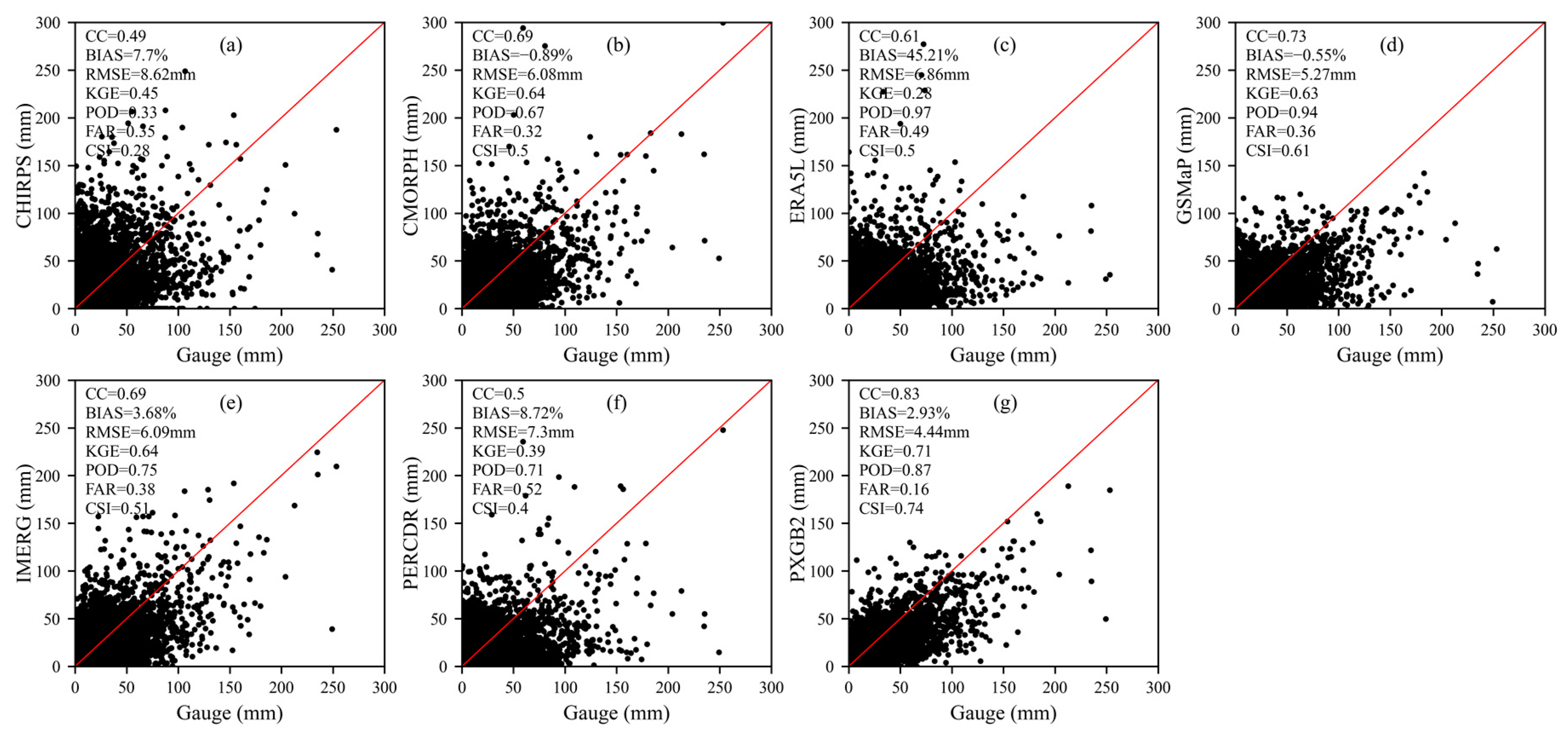
The daily precipitation extracted from multiple MSPs is compared with rain gauges. Figure 2 shows the scatterplots of seven products and their statistical metrics. The statistical metrics are obtained from the average of all rain gauges. The results show that the overall performance of PXGB2 is the best, while CHIRPS and PERCDR exhibit relatively poor performance. The outperformance of PXGB2 is attributed to its combination of the strengths of various precipitation products. However, the inferiority of CHIRPS and PERCDR may be that they incorporate only IR signals and not MW signals [13].

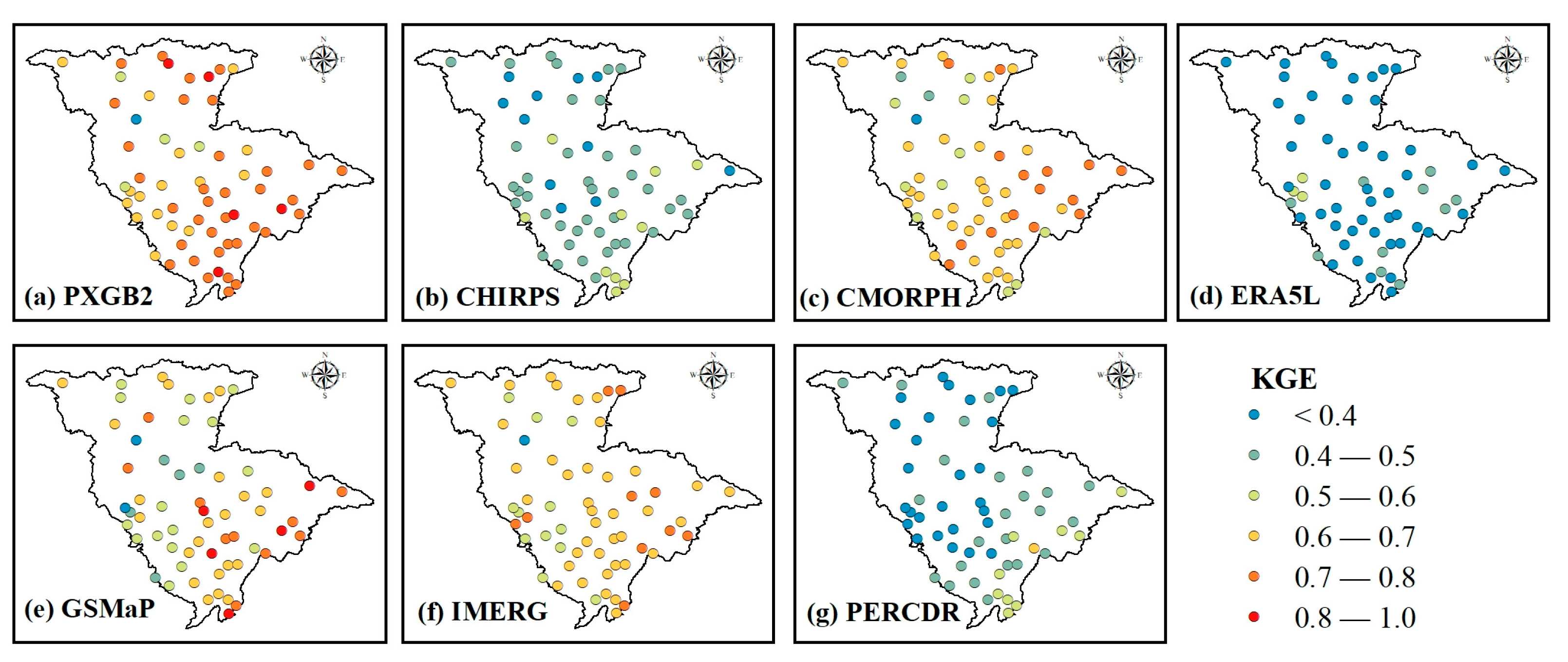
For continuous metrics, PXGB2 (Figure 2g) has a strong correlation (i.e., CC > 0.8) with gauge observations (CC = 0.83), followed by GSMaP (CC = 0.73). CHIRPS (Figure 2a) and PERCDR (Figure 2f) are more discrete and deviate from the reference line, with a CC of 0.49 and 0.5, respectively. Most MSPs overestimate the precipitation amounts, among which ERA5L has the largest overestimation by 45.21%. GSMaP and CMORPH show negligible underestimation, with BIAS of −0.55% and −0.89%, respectively. Regarding KGE and RMSE, PXGB2 has the highest KGE (0.71) and lowest RMSE (4.44 mm). GSMaP achieves the better RMSE (5.27 mm) with second ranking. IMERG and CMORPH have the same KGE (0.64). Figure 3 shows the spatial distribution of KGE for MSPs; it exhibits that there is a spatial variation in precipitation products. The KGE in the northwest part of the basin is worse than that in the southeast part of the basin, partly because the topography in the upper part of the basin is more complex.

For precipitation detection efficiency, except for CHIRPS, other products can capture precipitation occurrence well. The POD of MSPs ranges between 0.33 and 0.97. ERA5L (0.97) (Figure 2c) has the highest POD, followed by GSMaP (0.94) and PXGB2 (0.87). In terms of FAR, PXGB2 and PERCDR exhibit the best (0.16) and worst (0.52) values, respectively, indicating that the degree of false positives about precipitation is acceptable for most products. The CSI of each product has similar performance rankings to that of FAR. Although ERA5L performs better in POD, it has a poor FAR value (0.49). This implies many precipitation events have been falsely reported by ERA5L, which is also the main reason for its significant overestimation of precipitation amounts.

To facilitate the subsequent analysis of the impact of precipitation accuracy on hydrological simulation, the evaluation results of the MSPs in calibration (2001–2004) and validation (2005–2006) periods are summarized in

Table 4. The evaluation metrics of MSPs in calibration (2001–2004) and validation (2005–2006) periods. The unit of RMSE is mm.

Period	Metrics	CHIRPS	CMORPH	ERA5L	GSMaP	IMERG	PERCDR	PXGB2
Calibration	CC	0.48	0.69	0.63	0.74	0.68	0.49	0.83
	BIAS (%)	8.74	−0.31	51.05	1.53	5.17	10.54	4.20
	RMSE	8.74	6.09	6.89	5.20	6.16	7.42	4.40
	KGE	0.43	0.64	0.25	0.64	0.64	0.38	0.72
Validation	CC	0.50	0.70	0.60	0.72	0.70	0.53	0.83
	BIAS (%)	6.63	−1.49	34.84	−3.81	1.31	6.17	1.14
	RMSE	8.30	5.99	6.75	5.31	5.91	7.00	4.47
	KGE	0.46	0.64	0.32	0.59	0.64	0.39	0.69

. The general quality of MSPs is relatively stable in the calibration and validation periods. The daily CC and KGE of each product range between 0–0.04 and 0–0.07, respectively. Among all MSPs, ERA5L has the most significant accuracy variation between the two periods. For example, in calibration and validation periods, the BIAS of ERA5L is 51.05% and 34.84%, respectively. To sum up, most MSPs have similar performance in different years, which provides stable inputs for the streamflow simulation of hydrological models and avoids additional errors caused by data accuracy fluctuation.

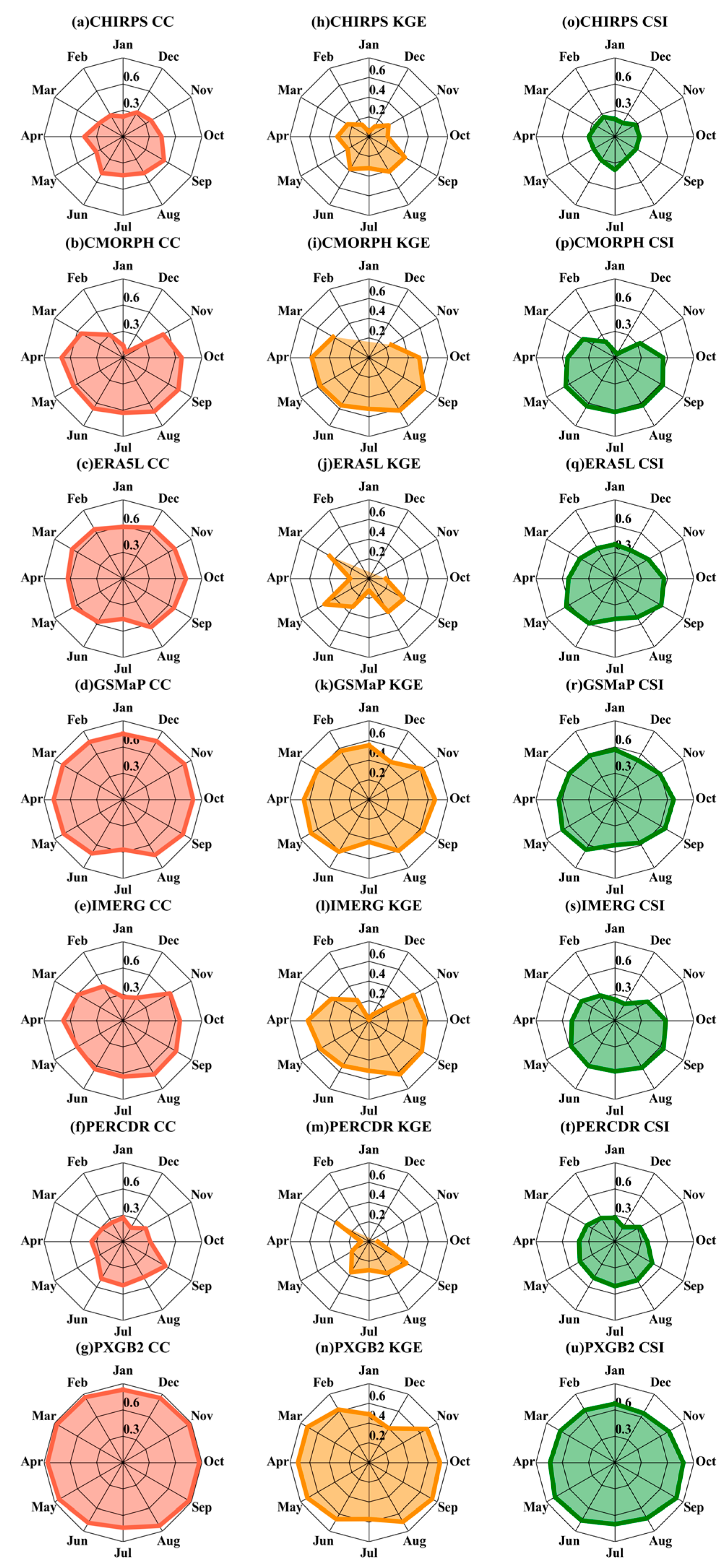
Figure 4 illustrates the CC, KGE, and CSI of MSPs in twelve months for analyzing their intra-annual distribution characteristics. In Figure 4, a month without border lines indicates a negative metric in that month, for example, the KGE of CMORPH (Figure 4i) in January, February, and December. It can be seen intuitively that PXGB2 and GSMaP occupy a larger area of the circle, which means they perform better each month and have relatively small accuracy fluctuations within the year. However, most MSPs have an unbalanced accuracy distribution throughout the year. For CC (Figure 4a–g), CHIRPS, CMORPH, IMERG, and PERCDR have poor performance in winter, while the poorest value of the other three products is discovered in July. CMORPH (Figure 4b) has the largest amplitude of fluctuation, with CC ranging from 0.07 (Dec) to 0.73 (Sep), followed by IMERG (0.27–0.71) (Figure 4e). In terms of KGE (Figure 4h–n), all products perform worst in winter than in spring and summer, especially the case for CMORPH, ERA5L, and PERCDR, whose KGE is negative throughout the winter. The CSI (Figure 4o–u) shows a similar trend to CC. The CSI of PXGB2 is the highest and is between 0.65 to 0.81. GSMaP (0.52–0.69) and ERA5L (0.37–0.64) take the second and third places, respectively. However, the variation of CHIRPS (0.18–0.38) and CMORPH (0.05–0.63) between each month is significant.

3.1.2. Basin Scale

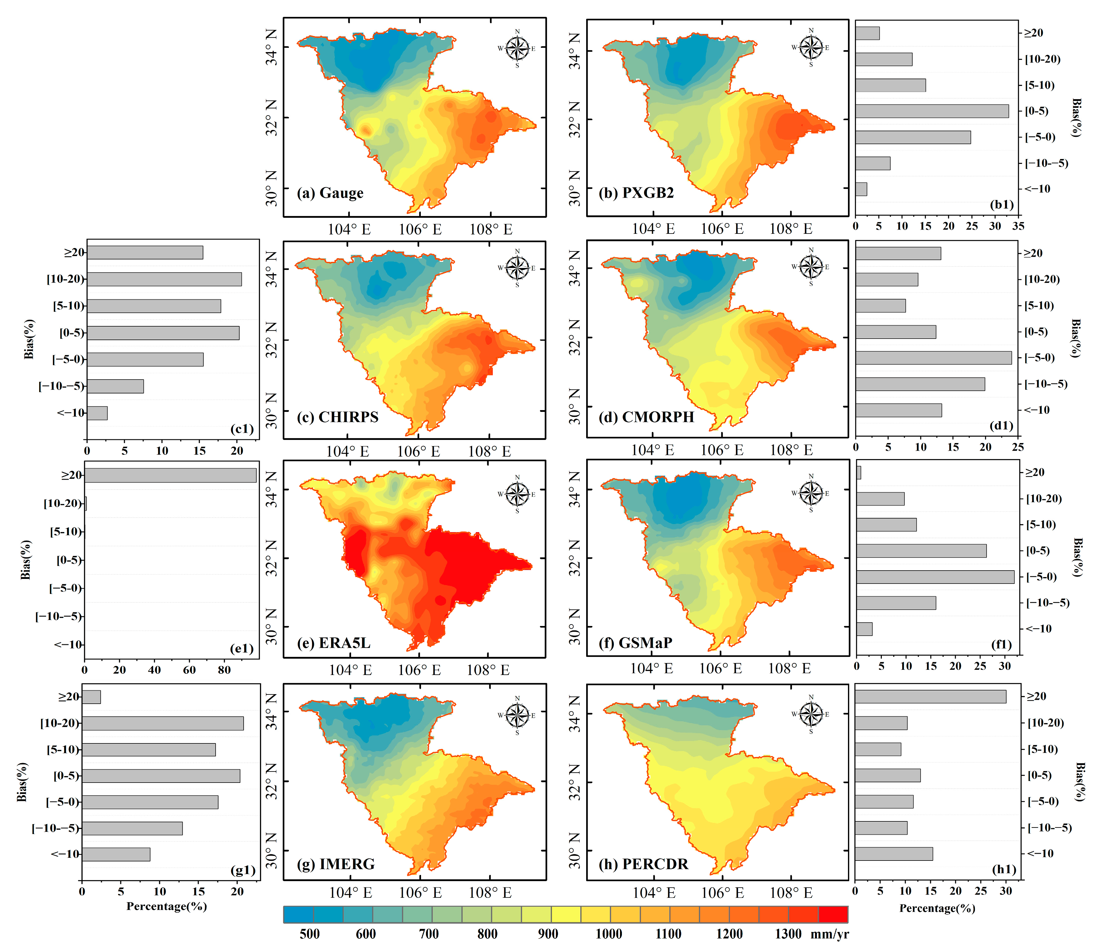
The spatial and bias distribution characteristics of precipitation products from 2001 to 2006 at the basin scale are analyzed by comparing the MSPs with the areal gauge observations (Figure 5). All the MSPs (Figure 5b–h) show a similar spatial pattern, with the precipitation increasing from the northwest to the southeast of the JLR basin, which agrees with gauge observations (Figure 5a). In terms of the average annual precipitation, ERA5L (1280.9 mm) considerably overestimates the precipitation of the entire basin, with 98.3% of grids overestimating by more than 20% (Figure 5e,(e1)). In addition, the bias of CHIRPS (Figure 5(c1)) and PERCDR (Figure 5(h1)) is mainly distributed to large positive values. The precipitation amounts of CMORPH (842.4 mm) and GSMaP (837.8 mm) are closer to gauge observations (838.5 mm), followed by IMERG (850.1 mm) and PXGB2 (858.7 mm). However, through the detailed analysis of precipitation distribution, CMORPH (Figure 5d) and IMERG (Figure 5e) overestimate the precipitation of the northwest part of the basin while underestimating the middle part of the basin. The proportion of grids with biases within ±5% is 37.9% for IMERG (Figure 5(g1)), 36.4% for CMORPH (Figure 5(d1)), 58.1% for GSMaP (Figure 5(f1)), and 57.7% for PXGB2 (Figure 5(b1)). Therefore, their better precipitation amount may be because the positive and negative biases are cancelled out in the spatial average of the entire basin. By comparison, GSMaP and PXGB2 more resemble gauge observations with relatively minor biases.

The annual precipitation of the MSPs for each year is also examined in

Table 5. The annual precipitation (mm) of gauge observations and MSPs from 2001 to 2006 at the basin scale.

Period	Gauge	CHIRPS	CMORPH	ERA5L	GSMaP	IMERG	PERCDR	PXGB2
Average annual	838.5	889.8	842.4	1280.9	837.8	850.1	886.7	858.7
2001	765.2	806.8	747.7	1297.4	743.7	776.9	817.8	778.9
2002	753.1	844.2	810.9	1198.9	768.8	792.5	875.0	797.8
2003	958.8	1038.1	961.4	1498.5	985.3	973.3	999.4	989.2
2004	854.1	870.6	835.8	1294.1	881.7	888.4	884.5	886.4
2005	963.3	948.7	966.0	1343.9	930.9	934.8	928.0	970.1
2006	736.4	830.4	732.7	1052.7	716.6	734.5	815.5	729.9

to investigate the inter-annual variability of precipitation. The annual precipitation ranges from 736.4 mm to 963.3 mm; the lowest and largest values appear in 2002 and 2005, respectively. All the MSPs can reproduce the interannual precipitation pattern from 2001 to 2006. The MSPs perform steadily each year and are characterized by little variability. However, the precipitation of ERA5L in 2001 is significantly overestimated by 70%, far more than 40% in 2005, which may be further reflected in the hydrological simulation.

3.2. Evaluation and Comparison Streamflow Simulation

3.2.1. Streamflow Simulation under Scenario I: Gauge-Based Calibration Parameters

In Scenario I, the streamflow of all the precipitation products in the calibration and validation periods is simulated using the gauge-calibrated parameters.

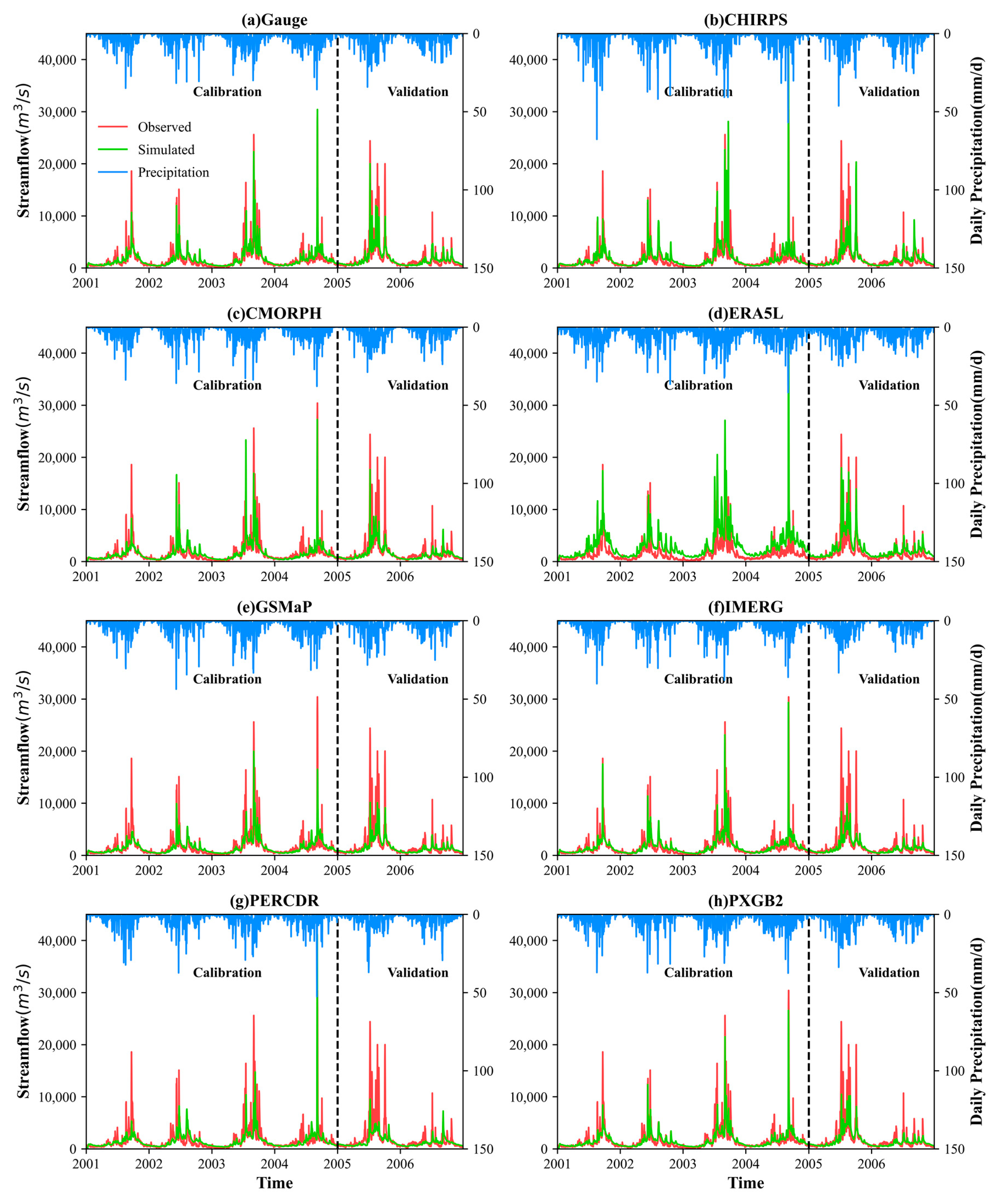
Figure 6 depicts the observed and simulated daily streamflow based on different precipitation products in the JLR basin.

Table 6. Performance of streamflow simulation rain gauges and seven MSPs under scenario I.

Metrics	Gauge	CHIRPS	CMORPH	IMERG	GSMaP	ERA5L	PERCDR	PXGB2
Calibration period (2001–2004)
R2	0.80	0.55	0.63	0.65	0.68	0.75	0.46	0.75
NSE	0.79	0.44	0.63	0.65	0.65	0.13	0.46	0.73
KGE	0.78	0.73	0.72	0.70	0.64	0.10	0.62	0.70
BIAS (%)	−0.02	7.28	−4.99	−0.97	−7.49	85.81	−9.37	−3.14
Validation period (2005–2006)
R2	0.82	0.66	0.65	0.61	0.66	0.76	0.55	0.71
NSE	0.77	0.64	0.58	0.51	0.54	0.72	0.42	0.61
KGE	0.72	0.68	0.59	0.52	0.53	0.52	0.43	0.60
BIAS (%)	−7.65	−7.65	−19.18	−20.18	−20.62	30.66	−25.79	−17.08
Entire period (2001–2006)
R2	0.80	0.56	0.62	0.61	0.66	0.70	0.45	0.73
NSE	0.79	0.52	0.61	0.60	0.61	0.35	0.44	0.69
KGE	0.76	0.74	0.68	0.65	0.61	0.27	0.56	0.67
BIAS (%)	−2.75	1.93	−10.07	−7.85	−12.19	66.07	−15.21	−8.13

summarizes the statistical results of the simulated streamflow in the calibration, validation, and entire periods. In general, the simulation could capture the characteristics of streamflow variation intra- and inter-annually. The streamflow simulated by gauge observations (Figure 6a) exhibits the best performance. It has the highest R² (0.8 and 0.82), NSE (0.79 and 0.77), KGE (0.78 and 0.72), and smaller BIAS (−0.02% and −7.65%) for the calibration and validation periods. Although some peak flows (Figure 6a) are underestimated, their occurrence timing and pattern can be well reproduced by the gauge-based simulated streamflow. The results indicate that the BTOP model is reliable and robust in the JLR basin and is suitable for studying the hydrological utility of different products.

As for the seven MSPs, in the calibration period, the simulation of PXGB2 achieves the best performance compared with other MSPs, with the largest R² of 0.75, NSE of 0.73, and a relatively satisfactory KGE of 0.70. GSMaP and IMERG have comparable NSE values (both are 0.65), while IMERG has a higher KGE (0.7) and the smallest BIAS (−0.97%). CMORPH has the acceptance performance with a better KGE (0.72). Although CHIRPS-based simulated streamflow has relatively lower R² (0.55) and NSE (0.44), it obtains the highest KGE (0.73). A similar situation is more pronounced in ERA5L. ERA5L has the best R² (0.75) and the worst NSE (0.13) and KGE (0.10). This suggests that only using a single diagnostic metric cannot sufficiently reflect the capability of streamflow simulation. Multiple hydrological metrics with different purposes should be used for evaluation. Moreover, ERA5L (Figure 6d) significantly overvalues the streamflow, especially in spring and autumn. Apart from ERA5L and CHIRPS, other MSPs cause the underestimation of the simulated streamflow, with the magnitude ranging from −9.37% to −0.97%. For the validation period, the reliability of the simulated streamflow is generally inferior to that of the calibration period, except for ERA5L with the highest NSE (0.72) and R² (0.76). This may be caused by the accuracy difference of ERA5L between the two periods (Table 4). Regarding NSE, the simulation performance of the MSPs is PXGB2 (0.61), CMORPH (0.58), GSMaP (0.54), IMERG (0.51), and PERCDR (0.42) in descending order. Throughout the entire period, PXGB2 maintains the best streamflow simulation performance, followed by GSMaP and CMORPH. The results demonstrate that the model calibrated based on gauge observations can be directly driven by other suitable precipitation sources to obtain reliable streamflow.

The exceedance probability (Figure 7) is employed to examine the ability of MSPs to capture the flow of different magnitudes. The flow duration curve (FDC) is divided into three segments, including the high-flow segment (probabilities lower than 5%), midsegment (probabilities between 20% and 70%), and low-flow segment (probabilities larger than 70%) [61,62]. Overall, the FDC (Figure 7a) from all the simulated results matches well with the observed curve in the entire probability except for a considerable overestimation of ERA5L. In high-flow (Figure 7b), ERA5L is more in line with the observed streamflow when frequencies are less than 2%. Other MSPs underestimate the high flow, of which PERCDR-based simulations yield the most significant underestimation magnitude. The higher accuracy is mainly concentrated in the midsegment, and GSMaP, IMERG, and CMORPH perform better in this segment. In low-flow, the overestimation gradually increases when probabilities are larger than 85% and the streamflow simulated by CMORPH presents the best performance. It can be concluded that the biases in streamflow simulation mainly come from high-flow and low-flow. The high-flow represents the basin’s response to heavy precipitation events. The low-flow is related to the long-term sustainability of the streamflow and is affected by the baseflow and evapotranspiration during dry periods [57], which is also associated with the soil properties and temperature of the basin. The capture ability of hydrological signatures is not only dependent on precipitation but is also affected by other environmental information.

3.2.2. Streamflow Simulation under Scenario II: Product-Specific Calibration Parameters

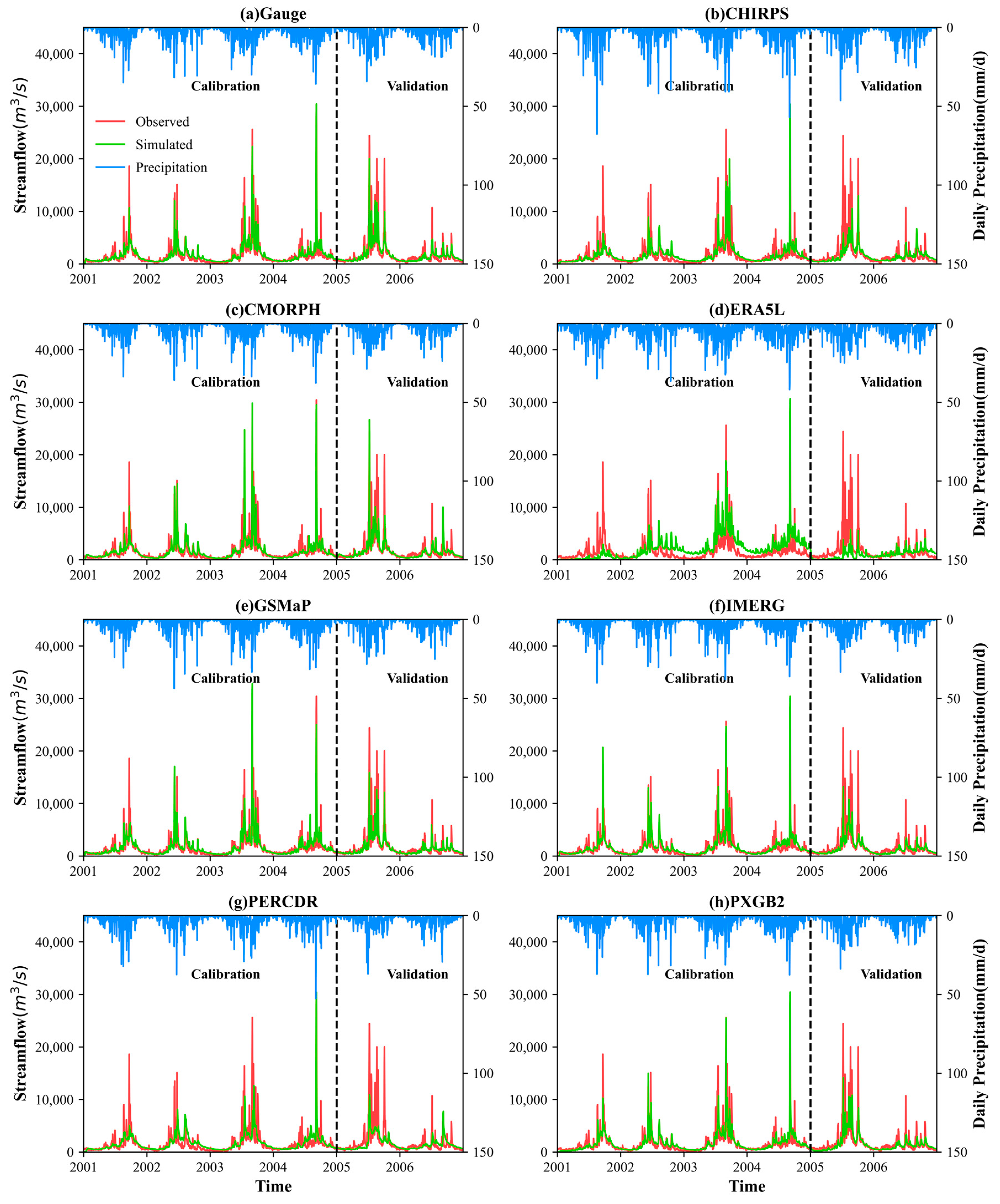
In Scenario II, the BTOP model is separately recalibrated and validated by each MSP.

Table 7. Performance of daily streamflow simulations of seven MSPs under scenario II.

Metrics	CHIRPS	CMORPH	IMERG	GSMaP	ERA5L	PERCDR	PXGB2
Calibration period (2001–2004)
R2	0.58	0.67	0.71	0.77	0.52	0.50	0.75
NSE	0.58	0.66	0.70	0.77	0.43	0.50	0.75
KGE	0.68	0.80	0.80	0.83	0.49	0.60	0.79
BIAS (%)	0.01	−0.03	0.00	−0.01	31.20	0.00	0.03
Validation period (2005–2006)
R2	0.55	0.61	0.61	0.81	0.25	0.48	0.69
NSE	0.50	0.60	0.54	0.72	0.13	0.43	0.63
KGE	0.53	0.70	0.58	0.68	0.20	0.47	0.66
BIAS (%)	−14.00	−11.29	−19.78	−16.96	−43.20	−18.50	−17.30
Entire period (2001–2006)
R2	0.55	0.64	0.65	0.76	0.36	0.48	0.71
NSE	0.55	0.64	0.64	0.75	0.32	0.47	0.71
KGE	0.63	0.77	0.74	0.79	0.53	0.56	0.75
BIAS (%)	−5.01	−4.06	−7.08	−6.08	4.56	−6.62	−6.18

and Figure 8 illustrate the streamflow of MSPs simulated using product-specific calibration parameters. The results show that the general performance of the simulations under Scenario II is significantly improved compared with Scenario I, especially for GSMaP, CHIRPS, and ERA5L. The results suggest that the model calibration plays an essential role in hydrological modeling, which can reduce the influence of precipitation error on hydrological simulation to a certain extent. The simulated streamflow well reflects the rising and falling trend of the observed streamflow. For the calibration period, GSMaP performs best with the highest R² (0.77), NSE (0.77), KGE (0.83), and lower BIAS (−0.01%). Although PXGB2 is the best product in precipitation evaluation, the PXGB2-based streamflow ranks second and has the better R² (0.75), NSE (0.75), and KGE (0.79). Similar results also occur between CHIRPS and PERCDR (Figure 2). This phenomenon reveals that the products with best performance do not necessarily produce the best-simulated streamflow. After recalibration, the bias of the simulated streamflow is largely narrowed. Except for 31.2% of ERA5L, the BIAS of the other MSPs could be negligible. For the validation period, the performance ranking of all the MSPs is slightly different from the calibration period. CMORPH has the highest KGE (0.7) and the lowest BIAS (−11.29%). The streamflow forced by IMERG (NSE = 0.54) is inferior to CMORPH (NSE = 0.6), which is contrary to the calibration period. Moreover, the accuracy deterioration of ERA5L is significant, with NSE dropping from 0.43 to 0.13. The significant discrepancy may be caused by the precision differences of ERA5L between the calibration and validation periods. Moreover, all MSPs underestimate the streamflow with BIAS ranging from −43.20% to −11.29%, which is larger than the calibration period. This is mainly because the mean observed streamflow in the calibration period is 1614.62 m³/s, whereas it is 1832.72 m³/s in the validation period, about 13.5% higher than the former. The transferability of the model parameters is related to the nonstationary climatic conditions. In other words, the model calibrated in relatively drier climate conditions may suffer from some uncertainties when applied in wetter periods. For the entire period, the R², NSE, and KGE of GSMaP and PXGB2 are larger than 0.7, implying that their performance is relatively balanced in all the aspects of streamflow simulation.

The exceedance probabilities (Figure 9a) of the simulated streamflow under scenario II are closer to the observed curve than under scenario I. All the MSP-based simulations underestimate the high-flow (Figure 9b) and overestimate the mid-flow when probabilities are between 20% and 50% (Figure 9c). CMORPH can better capture the flood peak with probabilities lower than 1%, mainly reflected in 2002 and 2004 (Figure 7c). There is considerable underestimation in ERA5L when probabilities are larger than 75%, contributing most to the overall streamflow bias. In low-flow, CHIRPS and PERCDR always overestimate streamflow while other MSPs overvalue when probabilities are less than 85%. The results reveal that each product has different capacities for various flow characteristics, and no one product can well capture the details of all moments. Therefore, suitable precipitation products should be selected according to specific needs, such as long-term streamflow or flood simulation.

3.3. Uncertainty Analysis of Hydrological Simulation

The relative importance of precipitation products, model parameters, and their interaction in hydrological simulation is qualified using the ANOVA method. In this study, due to the influence of the initial conditions of the model, the simulated streamflow in the initial period is unstable, especially in the case of a single simulation without parameter optimization. Therefore, the results of variance decomposition are based on the daily streamflow from 2002 to 2006 under different combinations of parameters and precipitation products to ensure the reliability of the analysis results.

Figure 10 displays the contribution ratio of the three sources to the total uncertainty of the streamflow simulation, respectively. The results show that the average contribution of precipitation products is the largest, with the ratio of 59%, indicating that precipitation products have the greatest impact on streamflow in this study. The effects of model parameters and their interaction account for 25% and 16%, respectively. In addition, the intra-annual distribution of their contribution has obvious characteristics. The interaction exhibits a higher contribution in June to September, which even exceeds the contribution of precipitation products in some flood events. However, it occupies a smaller contribution in winter (December to February), which is consistent with the pattern of streamflow (Figure 6). Moreover, the model parameters contribute the most from June to September. For example, from July to September 2002, their contribution ratio is significantly higher than that of the precipitation products. This reveals that the distribution characteristics of the three uncertainties are also affected by the period. In comparison, the effect of the precipitation product on streamflow presents the opposite trend; it is more significant in spring and winter than in summer and autumn.

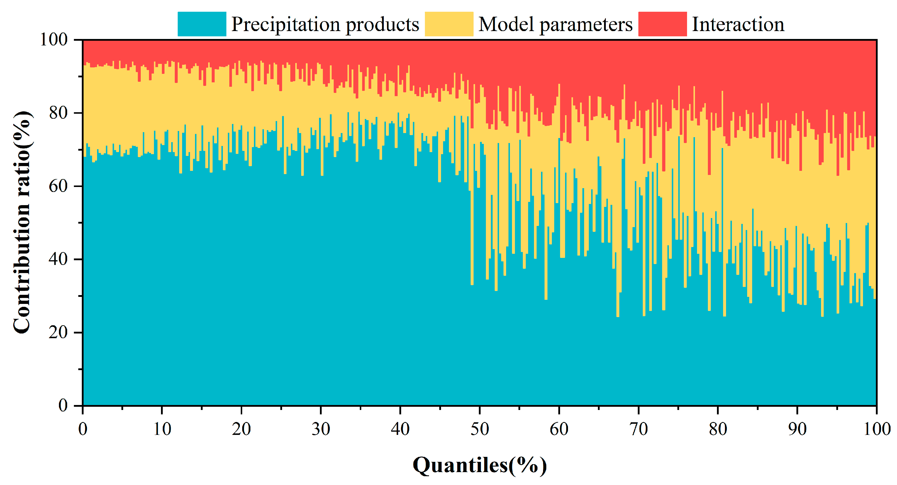
Figure 11 shows their contribution in different quantiles. It ranks the daily streamflow values in descending order. According to the exceedance probabilities in Section 4.2, the low, medium, and high flows correspond to the streamflow below the 30%, 30−95%, and above the 95% quantiles, respectively. In low flow, precipitation products, parameters, and their interaction contribute 71%, 21%, and 8% to the total uncertainty. The low flow mainly occurs in winter and early spring and is dominated by baseflow. Therefore, the variation tendency in low flow is relatively stable. In medium flow, the importance of model parameters and their interaction gradually increases with the streamflow value, accounting for 26% and 19% of the total uncertainties, respectively. The medium flow concentrates in spring and late autumn. Its hydrological processes are relatively complex, and it can be largely disturbed by model parameters and their interaction. Moreover, in high flow, the model parameters (37%) contribute more than precipitation products (36%) to streamflow, becoming the most important source of uncertainties. The interaction effect (27%) has also enlarged. The high-flow of streamflow usually appears in summer and early autumn, which is largely affected by extreme precipitation. The results reveal that the uncertainty in heavy precipitation can be compensated by model parameters and their interactions.

Overall, the relative importance of precipitation products, model parameters, and their interaction to streamflow varies with season and magnitude. They affect streamflow simulation together, and a single factor cannot completely determine the accuracy of the hydrological simulation. In other words, the influence of each factor on streamflow is limited. The interaction factor cannot unlimitedly reduce or amplify the differences between precipitation products. For example, the streamflow of GSMaP and PXGB2 always outperforms PERCDR and ERA5L. Anyhow, considering the interaction between precipitation products and model parameters helps us better understand the errors in hydrological modeling. If the interaction is not considered, the uncertainty contribution of precipitation products and model parameters will be overestimated.

4. Discussion

4.1. Evaluation of MSPs and Its Uncertainties

In this study, the quality of precipitation products is evaluated against gauge observations at the grid and basin scales. Affected by the topography and climate [63], the accuracy of the same product varies significantly in different areas. In this study, the general quality of CMORPH is superior to PERCDR and CHIRPS. The poor performances of PERCDR and CHIRPS can be attributed to their data sources and retrieval processes. The primary information used in creating CHIRPS is satellite-based IR information and gauge observations from various sources [64]. The IR channel measures cloud top temperature, cirrus clouds, or decaying rainfall complexes with cold, but nonprecipitating systems can easily be mistaken for precipitation systems if the IR data alone are used. On the contrary, precipitation is not necessarily associated only with cold clouds [42]. Therefore, it is necessary to combine IR and PMW to improve precipitation detection. Moreover, the accuracy discrepancy of each precipitation product relates to whether it has undergone error correction. For example, GSMaP and CMORPH use the daily gauge-based data, and IMERG is based on monthly GPCC data. However, only a tiny fraction of the number of China’s International Exchange Stations is used in GPCC [44], and more available rain gauge observations are desirable for improving the performance of these products. Focusing on this study again, PXGB2 has alleviated the drawbacks of various precipitation products and exhibits excellent quality in all aspects.

The precipitation evaluation is also affected by many factors. The gauge observations as the benchmark are subject to multitudinous sources of uncertainty, including wind-induced bias, evaporation loss, and wetting loss [65,66]. Rain gauges likely underestimate the actual precipitation in different regions by varying degrees, and this underestimation is certainly not negligible. How to effectively reduce the error of rain gauges is a key problem to be considered in future research. In addition, precipitation products represent the average characteristic within a grid cell (e.g., 5 km × 5 km), while rain gauges describe the precipitation at a point scale. The spatial scale inconsistencies between them will bring additional uncertainties to comparison, especially in regions with complex topography [67]. Therefore, alternative methods, such as the hydrological model, can overcome the spatial scale discrepancy and can be employed to evaluate the applicability of precipitation products from another angle.

4.2. Hydrological Evaluation and Its Uncertainties

In the hydrological simulation, the forcing data, the model structure, and model parameters codetermine and affect the simulation results [68,69]. For forcing data, the relationship between precipitation accuracy and hydrological simulation is not straightforward. A poor precipitation product does not necessarily cause inferior simulated streamflow [31,32]. For example, in this study, CHIRPS with poor daily performance performs better in hydrological simulation during the validation period (Table 6). One possible reason is that the bias in CHIRPS is compensated for by the coalition of the model structure and calibrated parameters. Traditionally, the model parameters are calibrated based on rain gauges (i.e., scenario I) because such parameters can better characterize the natural hydrological characteristics of the basin [28]. The results in scenario I (Table 6, Figure 6) demonstrate that precipitation products incorporating more rain gauges could bring more benefits for streamflow simulation. In comparison, the model calibrated by specific products (i.e., Scenario II) could partially offset the streamflow biases caused by the precipitation product. However, parameters calibrated by biased precipitation may not sufficiently represent the basin’s features.

Despite the extensive work on MSPs and their hydrological uncertainties that has been performed in this study, some deficiencies still need to be improved. The study mainly focuses on the influence of precipitation products and model parameters on hydrological simulation but does not take model structure into account. Different hydrological models have diverse responses to the quality of precipitation products [27,40,41]. More hydrological models with different structures (including lumped, semi-distributed, and distributed models) should be employed and compared in future studies. In addition, the forcing data of the BTOP model are not limited to precipitation but also evapotranspiration, temperature, soil moisture, etc., which could affect hydrological processes (e.g., baseflow) to varying degrees [30,70,71]. Moreover, the short period is also another limitation of this study. Since long-term streamflow data are unavailable and the hydrological dynamics in recent years have been greatly influenced by human activities, only six years of a hydrological station are used for hydrological assessments. Finally, it should be emphasized that the findings of this study are solely based on a single basin hydrological station; further efforts should be made to collect the data of different climatic conditions in more regions for comparison.

5. Conclusions

This study evaluates seven precipitation products based on the gauge-based statistical method and the BTOP hydrological model over the JLR basin. Subsequently, the ANOVA method is used to disaggregate the uncertainty sources of streamflow simulation into precipitation products, model parameters, and their interaction. The main conclusions of this study are summarized as follows:

• Compared to gauge observations, ensembled and satellite-based products reflect better precipitation capture ability and precipitation intensity than the reanalysis products used in this study. They have a similar spatial variation trend to the observations and have significant accuracy differences within the year. Generally, PXGB2 presents the best performance with the highest CC of 0.83, KGE of 0.71, and CSI of 0.74, followed by GSMaP and IMERG.
• The simulation results using gauge-calibrated parameters show that the simulation forced by observation precipitation performs best in both calibration and validation periods due to the robustness of the model and the relatively dense rain gauges in the JLR basin. Among the seven MSPs, PXGB2 presents better simulation with the highest R² (0.73) and NSE (0.69), indicating that incorporating various precipitation information can effectively reduce the error caused by single sources. Generally, GSMaP, IMERG, and CMORPH show better hydrological performance than CHIRPS, PERCDR, and ERA5L.
• The model parameters calibrated based on individual products significantly enhance the simulation performance of most MSPs, suggesting that model calibration can mitigate the impact of precipitation errors on streamflow simulation. The simulations can better capture the variation trends of streamflow in both timing and magnitude. This improvement is most remarkable in GSMaP, with the largest R² (0.76), NSE (0.75), and KGE (0.79). The most suitable performance rankings of MSPs are GSMaP, PXGB2, CMORPH, IMERG, CHIRPS, PERCDR, and ERA5L, which are slightly different from the gauge-calibrated simulation results.
• The results based on the ANOVA method show that the precipitation products contribute most to the total uncertainty of streamflow simulation. The contribution ratio of precipitation products, model parameters, and their interactions is 59%, 25%, and 16% in this study, respectively, which is influenced by seasons and the magnitude of streamflow. Under the influence of interaction, it is easier to understand why good products may produce unsatisfactory results. The result demonstrates that an appropriate combination of precipitation products and model parameters is essential to produce a good streamflow simulation.

This study reveals new insights into the quality of precipitation products and their uncertainty in simulating streamflow in the JLR basin. It is beneficial for obtaining efficient hydrological simulation and could provide a scientific guideline for relevant studies. Meanwhile, the uncertainty assessment framework can also be applied to other areas.

References

1. Behrangi, A.; Khakbaz, B.; Jaw, T.C.; AghaKouchak, A.; Hsu, K.; Sorooshian, S. Hydrologic evaluation of satellite precipitation products over a mid-size basin. J. Hydrol. 2011, 397, 225–237. [Google Scholar] [CrossRef] [Green Version]
2. Ma, D.; Xu, Y.P.; Gu, H.; Zhu, Q.; Sun, Z.; Xuan, W. Role of satellite and reanalysis precipitation products in streamflow and sediment modeling over a typical alpine and gorge region in Southwest China. Sci. Total Environ. 2019, 685, 934–950. [Google Scholar] [CrossRef] [PubMed]
3. Awange, J.; Hu, K.; Khaki, M. The newly merged satellite remotely sensed, gauge and reanalysis-based Multi-Source Weighted-Ensemble Precipitation: Evaluation over Australia and Africa (1981–2016). Sci. Total Environ. 2019, 670, 448–465. [Google Scholar] [CrossRef] [PubMed]
4. Ma, Y.; Sun, X.; Chen, H.; Hong, Y.; Zhang, Y. A two-stage blending approach for merging multiple satellite precipitation estimates and rain gauge observations: An experiment in the northeastern Tibetan Plateau. Hydrol. Earth Syst. Sci. 2021, 25, 359–374. [Google Scholar] [CrossRef]
5. Sun, R.; Yuan, H.; Liu, X.; Jiang, X. Evaluation of the latest satellite–gauge precipitation products and their hydrologic applications over the Huaihe River basin. J. Hydrol. 2016, 536, 302–319. [Google Scholar] [CrossRef]
6. Gao, Z.; Huang, B.; Ma, Z.; Chen, X.; Qiu, J.; Liu, D. Comprehensive comparisons of state-of-the-art gridded precipitation estimates for hydrological applications over southern China. Remote Sens. 2020, 12, 3997. [Google Scholar] [CrossRef]
7. Hsu, K.L.; Gao, X.; Sorooshian, S.; Gupta, H. Precipitation Estimation from Remotely Sensed Information Using Artificial Neural Networks. J. Appl. Meteorol. 1997, 36, 1176–1190. [Google Scholar] [CrossRef]
8. Huffman, G.J.; Bolvin, D.T.; Nelkin, E.J.; Tan, J.K. Integrated Multi-satellite Retrievals for GPM (IMERG) Technical Documentation, NASA. 2019. Available online: https://gpm1.gesdisc.eosdis.nasa.gov/data/GPM_L3/GPM_3IMERGDF.06/ (accessed on 12 June 2022).
9. Kubota, T.; Shige, S.; Hashizume, H.; Aonashi, K.; Takahashi, N.; Seto, S.; Hirose, M.; Takayabu, Y.N.; Ushio, T.; Nakagawa, K.; et al. Global precipitation 30 map using satellite-borne microwave radiometers by the GSMaP project: Production and validation. IEEE Trans. Geosci. Remote 2007, 45, 2259–2275. [Google Scholar] [CrossRef]
10. Funk, C.; Peterson, P.; Landsfeld, M.; Pedreros, D.; Verdin, J.; Shukla, S.; Husak, G.; Rowland, J.; Harrison, L.; Hoell, A.; et al. The climate hazards infrared precipitation with stations–a new environmental record for monitoring extremes. Sci. Data 2015, 2, 150066. [Google Scholar] [CrossRef] [Green Version]
11. Rodell, M.; Houser, P.R.; Jambor, U.; Gottschalck, J.; Mitchell, K.; Meng, C.-J.; Arsenault, K.; Cosgrove, B.; Radakovich, J.; Bosilovich, M.; et al. The Global Land Data Assimilation System. Am. Meteorol. Soc. 2004, 85, 381–394. [Google Scholar] [CrossRef]
12. Wang, X.; Li, B.; Chen, Y.; Guo, H.; Wang, Y.; Lian, L. Applicability Evaluation of Multisource Satellite Precipitation Data for Hydrological Research in Arid Mountainous Areas. Remote Sens. 2020, 12, 2886. [Google Scholar] [CrossRef]
13. Lei, H.; Zhao, H.; Ao, T. Ground validation and error decomposition for six state-of-the-art satellite precipitation products over mainland China. Atmos. Res. 2022, 269, 106017. [Google Scholar] [CrossRef]
14. Xu, J.; Ma, Z.; Yan, S.; Peng, J. Do ERA5 and ERA5-land precipitation estimates outperform satellite-based precipitation products? A comprehensive comparison between state-of-the-art model-based and satellite-based precipitation products over mainland China. J. Hydrol. 2022, 605, 127353. [Google Scholar] [CrossRef]
15. Khandu; Awange, J.L.; Forootan, E. An evaluation of high-resolution gridded precipitation products over Bhutan (1998–2012). Int. J. Climatol. 2016, 36, 1067–1087. [Google Scholar] [CrossRef]
16. Duan, Z.; Liu, J.; Tuo, Y.; Chiogna, G.; Disse, M. Evaluation of eight high spatial resolution gridded precipitation products in Adige Basin (Italy) at multiple temporal and spatial scales. Sci. Total Environ. 2016, 573, 1536–1553. [Google Scholar] [CrossRef] [PubMed] [Green Version]
17. Tan, M.L.; Santo, H. Comparison of GPM IMERG, TMPA 3B42 and PERSIANN-CDR satellite precipitation products over Malaysia. Atmos. Res. 2018, 202, 63–76. [Google Scholar] [CrossRef]
18. Kim, J.; Han, H. Evaluation of the CMORPH high-resolution precipitation product for hydrological applications over South Korea. Atmos. Res. 2021, 258, 105650. [Google Scholar] [CrossRef]
19. Moazami, S.; Najafi, M.R. A comprehensive evaluation of GPM-IMERG V06 and MRMS with hourly ground-based precipitation observations across Canada. J. Hydrol. 2021, 594, 125929. [Google Scholar] [CrossRef]
20. Alemohammad, S.H.; McColl, K.A.; Konings, A.G.; Entekhabi, D.; Stoffelen, A. Characterization of precipitation product errors across the United States using multiplicative triple collocation. Hydrol. Earth Syst. Sci. 2015, 19, 3489–3503. [Google Scholar] [CrossRef] [Green Version]
21. Massari, C.; Crow, W.; Brocca, L. An assessment of the performance of global rainfall estimates without ground-based observations. Hydrol. Earth Syst. Sci. 2017, 21, 4347–4361. [Google Scholar] [CrossRef]
22. Wu, Y.; Guo, L.; Zheng, H.; Zhang, B.; Li, M. Hydroclimate assessment of gridded precipitation products for the Tibetan Plateau. Sci. Total Environ. 2019, 660, 1555–1564. [Google Scholar] [CrossRef] [PubMed]
23. Lei, H.; Li, H.; Zhao, H.; Ao, T.; Li, X. Comprehensive evaluation of satellite and reanalysis precipitation products over the eastern Tibetan plateau characterized by ahigh diversity of topographies. Atmos. Res. 2021, 259, 105661. [Google Scholar] [CrossRef]
24. Li, K.; Tian, F.; Khan, M.Y.A.; Xu, R.; He, Z.; Yang, L.; Lu, H.; Ma, Y. A high-accuracy rainfall dataset by merging multiple satellites and dense gauges over the southern Tibetan Plateau for 2014–2019 warm seasons. Earth Syst. Sci. Data 2021, 13, 5455–5467. [Google Scholar] [CrossRef]
25. Wild, A.; Chua, Z.-W.; Kuleshov, Y. Evaluating accuracy of satellite precipitation estimates over the South West Pacific. Remote Sens. 2021, 13, 3929. [Google Scholar] [CrossRef]
26. Wild, A.; Chua, Z.-W.; Kuleshov, Y. Triple Collocation Analysis of Satellite Precipitation Estimates over Australia. Remote Sens. 2022, 14, 2724. [Google Scholar] [CrossRef]
27. Jiang, L.; Bauer-Gottwein, P. How do GPM IMERG precipitation estimates perform as hydrological model forcing? Evaluation for 300 catchments across Mainland China. J. Hydrol. 2019, 572, 486–500. [Google Scholar] [CrossRef]
28. Su, J.; Li, X.; Ren, W.; Lü, H.; Zheng, D. How reliable are the satellite-based precipitation estimations in guiding hydrological modelling in South China? J. Hydrol. 2021, 602, 126705. [Google Scholar] [CrossRef]
29. Tian, W.; Liu, X.; Wang, K.; Bai, P.; Liang, K.; Liu, C. Evaluation of six precipitation products in the Mekong River Basin. Atmos. Res. 2021, 255, 105539. [Google Scholar] [CrossRef]
30. Dembélé, M.; Schaefli, B.; Van De Giesen, N.; Mariéthoz, G. Suitability of 17 gridded rainfall and temperature datasets for large-scale hydrological modelling in West Africa. Hydrol. Earth Syst. Sci. 2020, 24, 5379–5406. [Google Scholar] [CrossRef]
31. Qi, W.; Zhang, C.; Fu, G.; Sweetapple, C.; Zhou, H. Evaluation of global fine-resolution precipitation products and their uncertainty quantification in ensemble discharge simulations. Hydrol. Earth Syst. Sci. 2016, 20, 903–920. [Google Scholar] [CrossRef]
32. Baez-Villanueva, O.M.; Zambrano-Bigiarini, M.; Mendoza, P.A.; McNamara, I.; Beck, H.E.; Thurner, J.; Nauditt, A.; Ribbe, L.; Thinh, N.X. On the selection of precipitation products for the regionalisation of hydrological model parameters. Hydrol. Earth Syst. Sci. 2021, 25, 5805–5837. [Google Scholar] [CrossRef]
33. Satgé, F.; Pillot, B.; Roig, H.; Bonnet, M.P. Are gridded precipitation datasets a good option for streamflow simulation across the juruá river basin, amazon? J. Hydrol. 2021, 602, 126773. [Google Scholar] [CrossRef]
34. Renard, B.; Kavetski, D.; Kuczera, G.; Thyer, M.; Franks, S.W. Understanding predictive uncertainty in hydrologic modeling: The challenge of identifying input and structural errors. Water Resour. Res. 2010, 46, W05521. [Google Scholar] [CrossRef]
35. Huard, D.; Mailhot, A. A Bayesian perspective on input uncertainty in model calibration: Application to hydrological model “abc”. Water Resour. Res. 2006, 42, W07416. [Google Scholar] [CrossRef] [Green Version]
36. Sun, R.; Yuan, H.; Yang, Y. Using multiple satellite-gauge merged precipitation products ensemble for hydrologic uncertainty analysis over the Huaihe River basin. J. Hydrol. 2018, 566, 406–420. [Google Scholar] [CrossRef] [Green Version]
37. Hong, Y.; Hsu, K.L.; Moradkhani, H.; Sorooshian, S. Uncertainty quantification of satellite precipitation estimation and Monte Carlo assessment of the error propagation into hydrologic response. Water Resour. Res. 2006, 42, W08421. [Google Scholar] [CrossRef] [Green Version]
38. Mockler, E.M.; Chun, K.P.; Sapriza-Azuri, G.; Bruen, M.; Wheater, H.S. Assessing the relative importance of parameter and forcing uncertainty and their interactions in conceptual hydrological model simulations. Adv. Water Resour. 2016, 97, 299–313. [Google Scholar] [CrossRef]
39. Bosshard, T.; Carambia, M.; Goergen, K.; Kotlarski, S.; Krahe, P.; Zappa, M.; Schär, C. Quantifying uncertainty sources in an ensemble of hydrological climate-impact projections. Water Resour. Res. 2013, 49, 1523–1536. [Google Scholar] [CrossRef] [Green Version]
40. Ma, Q.; Xiong, L.; Liu, D.; Xu, C.Y.; Guo, S. Evaluating the temporal dynamics of uncertainty contribution from satellite precipitation input in rainfall-runoff modeling using the variance decomposition method. Remote Sens. 2018, 10, 1876. [Google Scholar] [CrossRef] [Green Version]
41. Zhou, S.; Wang, Y.; Li, Z.; Chang, J.; Guo, A. Quantifying the uncertainty interaction between the model input and structure on hydrological processes. Water Resour. Res. 2021, 35, 3915–3935. [Google Scholar] [CrossRef]
42. Joyce, R.; Janowiak, J.; Arkin, P.; Xie, P. CMORPH: A method that produces global precipitation estimates from passive microwave and infrared data at high spatial and temporal resolution. J. Hydrometeorol. 2004, 5, 487–503. [Google Scholar] [CrossRef]
43. Hersbach, H.; Bell, B.; Berrisford, P.; Hirahara, S.; Horányi, A.; Muñoz-Sabater, J.; Nicolas, J.; Peubey, C.; Radu, R.; Schepers, D.; et al. The ERA5 global reanalysis. Q. J. Roy Meteorol. Soc. 2020, 146, 1999–2049. [Google Scholar] [CrossRef]
44. Lei, H.; Zhao, H.; Ao, T. A two-step merging strategy for incorporating multi-source precipitation products and gauge observations using machine learning classification and regression over China. Hydrol. Earth Syst. Sci. 2022, 26, 2969–2995. [Google Scholar] [CrossRef]
45. Yuan, H.; Dai, Y.; Xiao, Z.; Ji, D.; Shangguan, W. Reprocessing the MODIS Leaf Area Index Products for Land Surface and Climate Modelling. Remote Sens. Environ. 2011, 115, 1171–1187. [Google Scholar] [CrossRef]
46. Martens, B.; Gonzalez Miralles, D.; Lievens, H.; Van Der Schalie, R.; De Jeu, R.A.M.; Fernández-Prieto, D.; Beck, H.E.; Dorigo, W.A.; Verhoest, N.E.C. GLEAM v3: Satellite-based land evaporation and root-zone soil moisture. Geosci. Model Dev. 2017, 10, 1903–1925. [Google Scholar] [CrossRef] [Green Version]
47. Takeuchi, K.; Ao, T.; Ishidaira, H. Introduction of block-wise use of TOPMODEL and Muskingum-Cunge method for the hydroenvironmental simulation of a large ungauged basin. Hydrol. Sci. J. 1999, 44, 633–646. [Google Scholar] [CrossRef]
48. Takeuchi, K.; Hapuarachchi, P.; Zhou, M.; Ishidaira, H.; Magome, J. A BTOP model to extend TOPMODEL for distributed hydrological simulation of large basins. Hydrol. Process. 2008, 22, 3236–3251. [Google Scholar] [CrossRef]
49. Ao, T.; Ishidaira, H.; Takeuchi, K. Study of distributed runoff simulation model based on block type TOPMODEL and Muskingum-Cunge method. Proc. Hydraulic Eng. 1999, 43, 7–12. [Google Scholar] [CrossRef]
50. Beven, K.J.; Kirkby, M.J. A physically based, variable contributing area model of basin hydrology. Hydrol. Sci. Bull. 1979, 24, 43–69. [Google Scholar] [CrossRef] [Green Version]
51. Masutani, K.; Magome, J. An Application of Modified Muskingum-Cunge Routing Method with Water Conservation Condition to a Distributed Runoff Model. J. Jpn. Soc. Hydrol. Water Res. 2009, 22, 294–300. [Google Scholar] [CrossRef] [Green Version]
52. Shuttleworth, W.J.; Wallace, J.S. Evaporation from sparse crops—An energy combination theory. Q. J. Roy Meteor Soc. 1985, 111, 839–855. [Google Scholar] [CrossRef]
53. Zhou, M.C.; Ishidaira, H.; Hapuarachchi, H.P.; Magome, J.; Kiem, A.S.; Takeuchi, K. Estimating potential evapotranspiration using the Shuttleworth-Wallace model and NOAA-AVHRR NDVI to feed the hydrological modeling over the Mekong River Basin. J. Hydrol. 2006, 327, 151–173. [Google Scholar] [CrossRef]
54. Georgievsky, M.; Ishidaira, H.; Takeuchi, K. Development of a distributed snow model coupled with a new method of degree-day factors estimation. Ann. J. Hydraul. Eng. JSCE 2006, 50, 49–54. [Google Scholar] [CrossRef]
55. Duan, Q.; Soroosh, S.; Vijai, G. Effective and efficient global optimization for conceptual rainfall-runoff models. Water Resour. Res. 1992, 28, 1015–1031. [Google Scholar] [CrossRef]
56. Yuan, F.; Wang, B.; Shi, C.; Cui, W.; Zhao, C.; Liu, Y.; Ren, L.; Zhang, L.; Zhu, Y.; Chen, T.; et al. Evaluation of hydrological utility of IMERG Final run V05 and TMPA 3B42V7 satellite precipitation products in the Yellow River source region, China. J. Hydrol. 2018, 567, 696–711. [Google Scholar] [CrossRef]
57. Bitew, M.M.; Gebremichael, M. Evaluation of satellite rainfall products through hydrologic simulation in a fully distributed hydrologic model. Water Resour. Res. 2011, 47. [Google Scholar] [CrossRef]
58. Tang, G.; Zeng, Z.; Long, D.; Guo, X.; Yong, B.; Zhang, W.; Hong, Y. Statistical and hydrological comparisons between TRMM and GPM level-3 products over a midlatitude basin: Is day-1 IMERG a good successor for TMPA 3B42V7? J. Hydrometeorol. 2016, 17, 121–137. [Google Scholar] [CrossRef]
59. Gao, Z.; Long, D.; Tang, G.; Zeng, C.; Huang, J.; Hong, Y. Assessing the potential of satellite-based precipitation estimates for flood frequency analysis in ungauged or poorly gauged tributaries of China’s Yangtze River basin. J. Hydrol. 2017, 550, 478–496. [Google Scholar] [CrossRef]
60. Senatore, A.; Fuoco, D.; Maiolo, M.; Mendicino, G.; Smiatek, G.; Kunstmann, H. Evaluating the uncertainty of climate model structure and bias correction on the hydrological impact of projected climate change in a Mediterranean catchment. J. Hydro-Reg. Stud. 2022, 42, 101120. [Google Scholar] [CrossRef]
61. Yilmaz, K.K.; Gupta, H.V.; Wagener, T. A process-based diagnostic approach to model evaluation: Application to the NWS distributed hydrologic model. Water Resour. Res. 2008, 44, W09417. [Google Scholar] [CrossRef]
62. Sahraei, S.; Asadzadeh, M.; Unduche, F. Signature-based multi-modelling and multi-objective calibration of hydrologic models: Application in flood forecasting for Canadian Prairies. J. Hydrol. 2020, 588, 125095. [Google Scholar] [CrossRef]
63. Xie, P.; Yatagai, A.; Chen, M.; Hayasaka, T.; Fukushima, Y.; Liu, C.; Yang, S. A Gauge-based analysis of daily precipitation over East Asia. J. Hydrometeorol. 2007, 8, 607–626. [Google Scholar] [CrossRef]
64. Funk, C.C.; Peterson, P.J.; Landsfeld, M.F.; Pedreros, D.H.; Verdin, J.P.; Rowland, J.D.; Romero, B.E.; Husak, G.J.; Michaelsen, J.C.; Verdin, A.P. A quasi-global precipitation time series for drought monitoring. U.S. Geol. Survey Data Ser. 2014, 832, 4p. [Google Scholar] [CrossRef] [Green Version]
65. Ye, B.; Yang, D.; Ding, Y.; Han, T.; Koike, T. A bias-corrected precipitation climatology for China. J. Hydrometeorol. 2004, 5, 1147–1160. [Google Scholar] [CrossRef]
66. Ma, J.; Li, H.; Wang, J.; Hao, X.; Shao, D.; Lei, H. Reducing the statistical distribution error in gridded precipitation data for the Tibetan Plateau. J. Hydrometeorol. 2020, 21, 2641–2654. [Google Scholar] [CrossRef]
67. Hong, Z.; Han, X.; Li, D.; Long, G.; Tang, J. Wang. Generation of an improved precipitation dataset from multi-source information over the Tibetan Plateau. J. Hydrometeor. 2021, 22, 1275–1295. [Google Scholar] [CrossRef]
68. Wang, Q.; Xia, J.; She, D.; Zhang, X.; Liu, J.; Zhang, Y. Assessment of four latest long-term satellite-based precipitation products in capturing the extreme precipitation and streamflow across a humid region of southern China. Atmos. Res. 2021, 257, 105554. [Google Scholar] [CrossRef]
69. Liu, Y.; Zheng, Y.; Li, W.; Zhou, T. Evaluating the performance of satellite-based precipitation products using gauge measurement and hydrological modeling: A case study in a dry basin of Northwest China. J. Hydrometeorol. 2022, 23, 541–559. [Google Scholar] [CrossRef]
70. Kunnath-Poovakka, A.; Ryu, D.; Renzullo, L.J.; George, B. The efficacy of calibrating hydrologic model using remotely sensed evapotranspiration and soil moisture for streamflow prediction. J. Hydrol. 2016, 535, 509–524. [Google Scholar] [CrossRef]
71. Dile, Y.T.; Ayana, E.K.; Worqlul, A.W.; Xie, H.; Srinivasan, R.; Lefore, N.; You, L.; Clarke, N. Evaluating satellite-based evapotranspiration estimates for hydrological applications in data-scarce regions: A case in Ethiopia. Sci. Total Environ. 2020, 743, 140702. [Google Scholar] [CrossRef]
Figure 1. The location and topography of the study area. (a) is the JLJ basin, (b) is the location of the JLJ basin in Yangtze River Basin, (c) is the location of the Yangtze River Basin in China.
Remotesensing 15 00213 g001
Figure 2. Scatterplots of the daily precipitation between Gauge and seven products at the grid scale. The red line is the 1:1 reference line. (a) is CHIRPS, (b) is CMORPH, (c) is ERA5L, (d) is GSMaP, (e) is IMEGR, (f) is PERCDR, (g) is PXGB2.
Remotesensing 15 00213 g002
Figure 3. The spatial distribution of KGE for precipitation products compared with rain gauges.
Remotesensing 15 00213 g003
Figure 4. The CC (ag), KGE (hn), and CSI (ou) for each month of MSPs from 2001 to 2006 in JLR basin. The range of KGE is (−∞, 1), and the negative value of KGE is not shown in the figure.
Remotesensing 15 00213 g004
Figure 5. The spatial distribution (ah) of annual precipitation for gauge observations and MSPs, and the bias distribution (b1h1) of MSPs.
Remotesensing 15 00213 g005
Figure 6. Comparison of observed and BTOP simulated daily streamflow using gauge observations and seven MSPs in calibration and validation periods under scenario I.
Remotesensing 15 00213 g006
Figure 7. Comparison of the exceedance probabilities of the observed and simulated daily streamflow during the whole period under scenario I. (a) all frequencies; (b) frequencies below 5%; (c) frequencies between 20% and 70%; (d) frequencies exceeding 70%.
Remotesensing 15 00213 g007
Figure 8. Comparison of observed and BTOP simulated daily streamflow using gauge observations and seven MSPs in calibration and validation periods under scenario II.
Remotesensing 15 00213 g008
Figure 9. Comparison of the exceedance probabilities of the observed and simulated daily streamflow during the whole period under scenario II.
Remotesensing 15 00213 g009
Figure 10. The contribution ratio (%) of the precipitation products, model parameters, and their interaction to the total uncertainty of the streamflow simulation at the daily scale.
Remotesensing 15 00213 g010
Figure 11. The contribution ratio (%) of the precipitation products, model parameters, and their interaction to the total uncertainty of the streamflow simulation at different quantiles.
Remotesensing 15 00213 g011