Automatic Segmentation of Bulk Material Heaps Using Color, Texture, and Topography from Aerial Data and Deep Learning-Based Computer Vision

Abstract

This article proposes a novel approach to segment instances of bulk material heaps in aerial data using deep learning-based computer vision and transfer learning to automate material inventory procedures in the construction-, mining-, and material-handling industry. The proposed method uses information about color, texture, and surface topography as input features for a supervised computer vision algorithm. The approach neither relies on hand-crafted assumptions on the general shape of heaps, nor does it solely rely on surface material type recognition. Therefore, the method is able to (1) segment heaps with “atypical” shapes, (2) segment heaps that stand on a surface made of the same material as the heap itself, (3) segment individual heaps of the same material type that border each other, and (4) differentiate between artificial heaps and other objects of similar shape like natural hills. To utilize well-established segmentation algorithms for raster-grid-based data structures, this study proposes a pre-processing step to remove all overhanging occlusions from a 3D surface scan and convert it into a 2.5D raster format. Preliminary results demonstrate the general feasibility of the approach. The average F1 score computed on the test set was 0.70 regarding object detection and 0.90 regarding the pixelwise segmentation.

1. Introduction

Monitoring bulk material quantities is an essential task in several industries including the construction-, mining-, waste-, and construction material industry. Material of a loose consistency like sand, gravel, or gangue is usually stored in the form of heaps. The volumes of those heaps are important parameters for process and inventory control (compare, e.g., [1,2,3,4,5]).

Traditionally, bulk material amounts are either measured in terms of weight [5] or the volumes are calculated when the material is transported in containers with known capacities (“truckload-and-bucket-count” [6]). On construction sites and construction material plant sites, in quarries or in open pit mines, bulk material is usually stored in the form of heaps, also referred to as stockpiles. While all those heaps are created essentially by pouring bulk material on the ground, the appearance and properties of both the heaps and their surroundings vary greatly. Heaps can either be placed with space in between them, border each other, or even overlap. The surrounding ground surface can either consist of the same material as some of the heaps or of a different material. It can be flat, tilted, even or uneven. Figure 1 shows point clouds of two construction material industry sites that contain bulk material heaps of various shapes, sizes, materials, and surroundings.

Several traditional methods exist to measure or estimate the volumes of bulk material heaps directly on site. A relatively inaccurate method estimates the volume of a stockpile based on a few reference measurements in combination with personal experience (“eyeballing method” [6]). Less error-prone, but also much more time-consuming, is the calculation of stockpile volumes based on point-wise measurements of the stockpile’s surfaces [5]. This, however, requires (1) a surveyor to walk on top of the material heap and (2) only allows for a rough approximation of the surface geometry, since a detailed measurement of the surface topography using a dense grid of sample points would be too time-consuming and therefore inefficient.

1.1. Using Remote Sensing Data for Bulk Material Volume Computation

Modern Sensor Technologies like LiDAR, data processing techniques like Structure from Motion (SfM), and flexible sensor platforms like unmanned aerial vehicles (UAV) offer more efficient ways to acquire detailed data about both the geometry and the visual appearance of the scanned surfaces (compare, e.g., [7,8]).

In the construction-, mining-, and material-handling industry, aerial data gathered via UAV and visual sensors is already widely used for a variety of planning and monitoring tasks. It is an increasingly common practice to compute properties like length, area, or volume from the acquired surface scan data instead of measuring or counting the objects or areas of interest directly on site (compare, e.g., [9,10,11]). Several studies specifically discuss the usage of those technologies to monitor bulk material volumes.

Kovanič et al. [4] compared stockpile volume computation based on aerial photogrammetry with results based on terrestrial laser scan (TSL) and confirmed that aerial photogrammetry is efficient, accurate, and fast.

Son et al. [6] proposed a method that integrates UAV-based laser scan data and TLS data. Their goal is to derive an optimal waste stockpile volume computation by fusing the two technologies. They also compared the suitability and accuracy of point clouds generated (1) via UAV-based laser scan, (2) TLS, and (3) a method that fused two technologies. They concluded that all three methods were suitable and produced similar results regarding the volume computation.

Alsayed et al. [12] discussed whether UAVs are suitable for bulk material volume estimation in confined spaces. The study was conducted in the context of an asphalt industry plant, where manual measurements of stockpiles in confined spaces pose a danger to the plant workers. They show that this approach allows for an increase in both measurement accuracy and safety.

A study that monitors volumes and changes in volumes in a slightly different context is presented by Park et al. [9]. The study presents a UAV-based earthwork management system in the context of high-rise building construction. It is concluded that UAV-based photogrammetry is a suitable and accurate method to monitor cut-and-fill volume and height difference between different points in time.

1.2. Bottleneck: Manual Data Processing Steps

While the acquisition of aerial surface scan data for monitoring and inventory purposes has proven to be valid in several studies and is already common practice in many industries, processing the acquired data usually involves manual tasks. One of the most fundamental tasks consists of “giving meaning” to the acquired surface scan data, e.g., by marking certain areas as being part of a certain object or category. This is usually performed manually by viewing and annotating the surface scan data in suitable GIS-, CAD-, or Point Cloud Viewer software.

To calculate the volumes of individual bulk material heaps based on digital surface models, the heaps must first be identified and isolated from the rest of the surface to allow for the computation of the enclosed volume. Tucci et al. [1] described in detail how this can be done manually using GIS and Point Cloud Processing software. The process includes two essential manual steps: (1) the removal of points that belong to “overhanging” objects like trees or cranes and (2) the segmentation of the individual stockpiles from the rest of the digital surface model by means of manually drawing polygons that mark the outlines of individual stockpiles. The necessity of those manual annotation steps so far stands in the way of a complete automation of bulk material inventories based on remote sensing data.

1.3. Proposed Method and Objective

This study proposes a novel approach to automate the segmentation of individual stockpiles using both color and surface geometry from aerial data as input features for a supervised computer vision algorithm. To enable the usage of well-established instance segmentation algorithms for image-like raster data, we proposed an additional pre-processing step that automatically removes overhanging points and converts the point cloud data into a 2.5D raster format. To achieve useful results despite the limited amount of available training data, the proposed method leverages a pre-trained neural network for transfer learning.

The goal of this study is to develop a stockpile segmentation method that neither relies on hand-crafted assumptions about the general shape of heaps nor on surface material recognition alone. The method should be able to (1) segment heaps with “atypical” shapes, (2) segment heaps that stand on a surface made of the same material as the heap itself, (3) segment individual heaps of the same material type that border each other, and (4) differentiate between artificial heaps and other objects of similar shape like natural hills. Figure 2 illustrates how the proposed method could constitute a central component of an automated bulk material inventory system.

The objective of this paper is to introduce the approach conceptually and to validate its feasibility via a demonstrator and real-world test data. The proposed method is put into context of existing methods and compared to them qualitatively. It is not within the scope of this paper to present comparative quantitative analysis of different settings and hyperparameters of the individual components of the proposed method. This is subject to further research.

1.4. Existing Approaches to Automate Stockpile Segmentation in Remote Sensing Data

Several approaches exist to automatically segment heaps of bulk material from remote sensing data like Point Clouds, DEMs, or Orthomosaics. Two categories of existing approaches are identified in the context of this study. Into category 1 fall methods that first perform semantic segmentation by assigning a categorical label to each pixel or point, optionally followed by a separate spatial clustering step to group individual heaps based on spatial distance. Those methods usually rely primarily on surface material recognition. Into category 2 fall methods that directly perform instance segmentation, meaning they detect individual heap instances and segment each heap “pixel/point-perfect” based on the input features without having to rely on spatial clustering to identify individual heaps.

While those approaches appear to yield good results for their respective specialized domain and/or environment, the following qualitative limitations appear to prevent them from being applicable for heap instance segmentation in other domains and/or for differently shaped heaps and environments. None of the approaches use information about both the visual surface appearance and the explicit surface topography as input features for their respective segmentation step. Methods that use only visual features appear to be unable to detect heaps that border each other or stand on a ground made of the same material as the heaps. The approach that uses only geometrical features, on the other hand, seems to depend on the heaps displaying a somewhat “typical”, predictable shape. Additionally, this approach may be prone to falsely detect other heap-like shaped objects.

The next two sections discuss the existing approaches. The first section lists approaches that first segment regions semantically based on the apparent surface material (in some cases followed by a clustering step); the second section discusses approaches that directly segment individual instances of bulk material heaps.

1.4.1. Approaches Based on Surface Material Recognition

Semantic segmentation of orthomosaics via deep learning was used by Jiang et al. [13] to detect piles of demolition debris (see Figure 3). The segmentation component itself assigns a binary label to each pixel in the orthomosaics to denote whether the pixel is part of demolition debris or not. The approach is reported to be relatively accurate with an Intersection-over-Union (IoU) score of 0.9. Consecutive/adjacent pixels that belong to the category “debris” are grouped together. Therefore, the method can identify individual heaps/agglomerations of debris if there is a large enough spatial distance between the areas that are occluded with debris.

However, based on the fact that the segmentation algorithm (1) does not take into account relative height as a feature and (2) individual heaps are grouped by means of spatial distance between areas that are covered with the same material type, it is assumed that the method would neither be able to detect individual bulk material heaps that consist of the same material and directly border each other, nor could it segment heaps that stand on a ground which is covered with the same material as the heaps themselves. The study also proposes to compute a DEM and Orthomosaics representation of a 3D point cloud. However, it does not include information derived from the DEM as features for the segmentation process. Additionally, it does not mention a step to remove possible occlusions like trees or cranes that might block the birds-eye view on potential stockpile areas.

Sivitskis et al. [14] detected slag material in satellite imagery using Mixed Tuned Match Filtering (MTMF) on multispectral image data. It was concluded that the proposed method shows an overall accuracy of 90%. Since this method is also primarily aimed to identify areas that are covered with material of a certain type and not to identify individual material heaps, it is expected to have the same limitations regarding heap instance segmentation as Jiang et al. [13].

An approach to recognize material heaps on RGB images in the context of a recycling plant by computing the amount of edges at a specific region of the image was proposed by Finkbeiner [15]. The approach follows from the claim that the recycling material displays many different and randomly distributed colors and shapes, and therefore a dense net of edges is apparent on the parts of the image that show the surface of the bulk material. Those edges are computed using the Canny Edge Detection algorithm [16], and consecutive regions of bulk material are identified using further image transformation and clustering steps. In principle, the method is analogous to semantic segmentation of regions based on the surface material followed by a spatial clustering step, thus it is expected to have the same limitations regarding stockpile instances segmentation as [13] and [14]. Additionally, it seems likely that the approach would not work in an environment where other surfaces also display “a lot of edges”, like, for example, vegetation or stony ground.

1.4.2. Approaches Based on Direct Segmentation of Individual Heap Instances

The following two studies propose methods to directly segment individual heap instances. The first study uses local geometric features of a point cloud representation, and the second study performs instance segmentation on individual RGB images directly on a drone-mounted edge device.

Yang et al. [5] proposed a method that extracts individual instances of stockpiles from 3D point cloud data based on Multi-Scale Directional Curvature (see Figure 4). The study is conducted in the context of coal stockpiles in mines, ports, and powerplants. The proposed algorithm extracts stockpiles by (1) identifying individual crests and (2) using a competitive growing strategy to locate the points that belong to the slope regions of the individual stockpiles. The average IoU score regarding the stockpile extraction is reported to be 93.5%, and the average precision of volume is 93.7%. While the method appears to be quite promising for areas where regular-shaped stockpiles stand free on a relatively even ground, it stands to reason that the method may perform less well in “less predictable” environments, where other objects or even parts of the ground also display a “heap-like” shape.

Kumar et al. [17] used deep learning-based instance segmentation together with a stereo camera and depth estimation on an edge device to calculate material volumes “on the fly”. The method was developed and tested to detect material heaps in open pit mines. Stockpiles were segmented on the instance level from 2D images. The depth detection was used to estimate the 3D shape of the segmented areas by computing a 3D point cloud of the scene captured in a single image based on estimated Euclidean distance and angle of response. The depth estimation therefore functions as a substitute for common distance measurement like LiDAR or methods that compute the 3D surface geometry based on multiple overlapping images from various angles like Structure from Motion (SfM); it is not used as input features to the segmentation algorithm. The method aims at scenarios where the volume computation task must be accomplished in a short time or in risk areas. While the authors conclude that the method is relatively fast and efficient, they also conclude that it is not very accurate in its current state and thus allows for quick volume estimation rather than for precise volume calculation.

1.4.3. Related Tasks

On a closely related topic, several studies aim not to segment individual stockpile instances, but individual grains of the bulk material, in order to classify the material and to compute properties like the grading curve. Further research could address approaches to combine such methods with the heap–instance–segmentation approach presented in this article.

A study that aims to automatically compute the gradation of rockfill material based on instance segmentation was presented by Fan et al. [18]. The proposed method segments individual grains (see Figure 5), and then computes the gradation based on the dimensions of those grains. The reported Average Prediction (AP) score was 0.934 and the IoU value was 0.879. They reported that the particle gradation detected by their proposed method had a good overall fitting effect with the actual gradation parameters.

Fan et al. [19] present a study that uses 3D point cloud segmentation to separate and extract individual riprap rocks from stockpiles to characterize their shape and size. The method is reported to yield accurate results, with a Mean Percentage Error of 2% regarding the predicted grain volumes.

2. Materials and Methods

2.1. Data Source and Industrial Context

In the scope of this study, the proposed method was developed and tested for bulk material heaps in the context of asphalt mixing plants, quarries, and construction material recycling- and storage-sites.

The sites used as test and training data are operated by subsidiaries of the VINCI group. On those sites, material inventories have been performed periodically over the last years using UAVs and Photogrammetry to acquire surface scan data. Stockpile volumes were computed based on those scans by (1) manually drawing boundary polygons around the stockpiles and (2) evaluating the volume using established approximation methods which use the interpolated heights from two DEMs, one representing the stockpile’s surfaces and the other one representing the ground on which the stockpiles rest. Those inventories “labelled” training data as a side-effect, since the georeferenced boundary polygons can be automatically converted into instance segmentation masks. In total, 18 sites were chosen in the scope of this study, 15 were used to train the instance segmentation model, and three were reserved to test the performance of the trained model on previously unseen sites. The proposed method is also expected to be applicable to other industries like open pit mining due to the similarity regarding the respective bulk materials and the general appearance of the surrounding.

The current implementation of the prototype does not distinguish between different types of bulk materials. This information was not part of the pre-labeled data created by the former inventory operations. This functionality, however, could be added in principle by differentiating between multiple stockpile classes during instance segmentation, or it could be added in form of a separate subsequent component that classifies detected heaps as a whole.

2.2. Methodology

“A million grains of sand is a heap of sand.

A heap of sand minus a grain is still a heap.

Thus 999,999 grains of sand are a heap.

A heap of sand minus a grain is still a heap.

Thus…

…

… a grain of sand is a heap.”

Based on “Sorites Paradox” [20]

Unlike a common interpretation of this “paradox”, in the context of this study, it is not stated to question the existence of heaps, but to illustrate that it is not that clear what exactly a “heap of bulk material” refers to. Just like there is no general definition for the minimum required number of grains in a heap, there is also no objective distinct border that separates, for instance, two heaps from one heap with two tips, or an irrelevant aggregation of loose material from a relevant stockpile. Unlike cars or sheep, a heap often does not have a clear distinct border or outline, especially if it stands on a ground that is occluded with the same material that constitutes the heap. These boundaries are fluid and always, to some extent, subjective. While it is possible to draw this boundary using hand-crafted thresholds for properties like volume, height, change in curvature, or a complex combination of those, the approach presented in this study aims to learn these boundaries from labeled examples, thus trying to replicate the intuition of a human on that subject.

For this purpose, a supervised deep learning-based computer vision algorithm was leveraged. The data presented to the algorithm contains information on both the surface appearance and the general shape of areas with potential stockpiles, therefore allowing to find “decision boundaries” based on any combination of those features.

2.2.1. Segmentation of 2.5D Raster- vs. 3D Set-Based Data Structures

The approach proposed in this article presents the surface scan data in a 2.5-dimensional raster grid format. This approach was chosen for the following reasons.

With regard to the use of deep learning algorithms for automatic segmentation of surface scan data, it makes a big difference whether the data is represented as an ordered grid, like in the case of digital images, or whether the data is represented as an unordered set, like it is commonly used to store 3D point clouds (compare, e.g., [21,22,23]). Well-established computer vision algorithms for image data, Convolutional Neural Networks (CNN), make use of the ordered raster grid structure. The spatial relation of local features in an image are vital for convolution operations in CNNs.

Set-based data structures are, by definition, permutation-invariant [22], meaning that the order of the points in the set does not matter. This makes feature extraction challenging for established deep learning models [24]. Addressing this challenge is still subject to ongoing research. Some approaches convert the point cloud data into a 3D raster grid-like format, like, e.g., a voxel grid, and others aim to operate on the set-based data structure directly [25]. Most of the latter approaches are based on the PointNet architecture presented by [22].

Apart from the matureness of the deep learning model itself, the amount of labelled open-source training data available for pretraining and the efficiency of the labelling process for new domain-specific data are also a relevant factor. Labelling instances on 2D images for instance-segmentation can be done relatively fast by drawing 2D polygons around the respective regions. In 3D, marking each point of a complex shape, like, e.g., a tree in a forest, by either selecting all relevant points or by drawing a 3D boundary shape around them, is often much more difficult and time-consuming. It also requires more complicated navigation in a 3D environment.

Those factors, together with the claim that all bulk material heap surfaces can be fully represented as 2.5D raster data, motivate the use of established 2D image segmentation algorithms on correspondingly pre-processed data instead of a direct segmentation of 3D point clouds.

2.2.2. Implications of Transfer Learning Regarding Input Channel Dimensionality

The segmentation component of the proposed method leverages the Mask-RCNN [26] instance segmentation model with pretrained weights using transfer learning [27]. Transfer learning is a technique widely used in supervised computer vision; the idea is to have the model learn general features like edges, contrast, etc., during pre-training from a large-scale dataset of a different domain (compare, e.g., [28,29]). This dataset is usually much larger and “cheaper”/easier to access than the domain-specific dataset. The weights resulting from the pre-training are used as a “starting-point” for the training on the domain-specific data [27]. This technique often has significant advantages regarding the required amount of new domain-specific training data and regarding the required computation time needed for training. The weights of the ResNet-50 backbone of the Mask-RCNN [26] model used in this study were pretrained on the COCO dataset [30], which consists of over 100.000 three-channel RGB color images.

A potential drawback of this approach in the context of the proposed stockpile segmentation method comes from the number of channels of the data in large-scale open-source image recognition datasets like MS COCO and ImageNet. Those datasets mostly consist of 3-channel RGB images, since this is the common format for digital imagery (Even though image formats like PNG allow for a fourth channel for transparency, this channel usually does not carry useful information for image recognition).

The raster images created from the 3D point cloud, however, contain information in four separate channels: three color channels plus the height values.

There are two basic options to deal with this issue: (1) changing the input layer of the model to allow for additional channels or (2) compressing the data from four channels into three channels. Both approaches have their potential caveats.

The first approach has the potential downside that each new channel in the input data requires a corresponding new channel in the convolutional filters of the input layer of the Mask-RCNN backbone. Since those filter channels did not exist during pretraining, their weights must be initialized “from scratch”, e.g., randomly or by copying them over from another filter channel. This changes the output of the first layer (the values, not the shape), which may make the filters in the subsequent layers less effective. While this effect is expected to fade out over time given enough domain-specific training data, it stands to reason that, in case of a relatively small training set, the model may perform better when being trained on a compressed three-channel view of the domain-specific four-channel data.

An alternative option to add additional input channels could be to use two instead of one pre-trained feature-extractors in parallel as the backbone for the Mask-RCNN model, each one with its own three-channel input. The feature maps produced by the two back models would then be combined before feeding them to subsequent stages of the model. The second feature-extractor could take, for example, a heatmap view of the height values as input, while the first one would input the corresponding RGB view. While this strategy seems promising to avoid the issues regarding the possible invalidation of the pre-trained weights mentioned above, it would require substantial changes to the model architecture.

The second approach—compressing the data from four or more channels into three channels—comes with the obvious downside of losing information during data compression. How much and which information is lost depends on the concrete compression mechanism (compare Section 2.4.4.).

A theoretical third option to avoid all the aforementioned issues would be to train the entire model from scratch. Given the limited amount of domain-specific training data available for this study, this approach does not seem reasonable in the light of existing research regarding the effectiveness of transfer learning in other domains (compare, e.g., [27,28,29]).

As stated in Section 1.3, the objective of this paper is to introduce the general concept of the proposed stockpile segmentation approach and to validate its general feasibility. It is not the goal to compare and optimize the various possible variations of the proposed pipeline’s components. Therefore, one single prototype with a single set of parameters and input features was implemented and evaluated in the current phase of the research. For this prototype, we decided to follow the strictly data-centric approach and chose the second option to adjust the input data instead of the model structure. Evaluating whether the information-loss during data compression outweighs the potential “damage” that might be done to the validity of the pre-trained weights is subject to further research. It is expected that this depends on the amount of available domain-specific training data, the information content of the additional channel, and the concrete implementation changes made to the model.

2.3. Proposed Pipeline

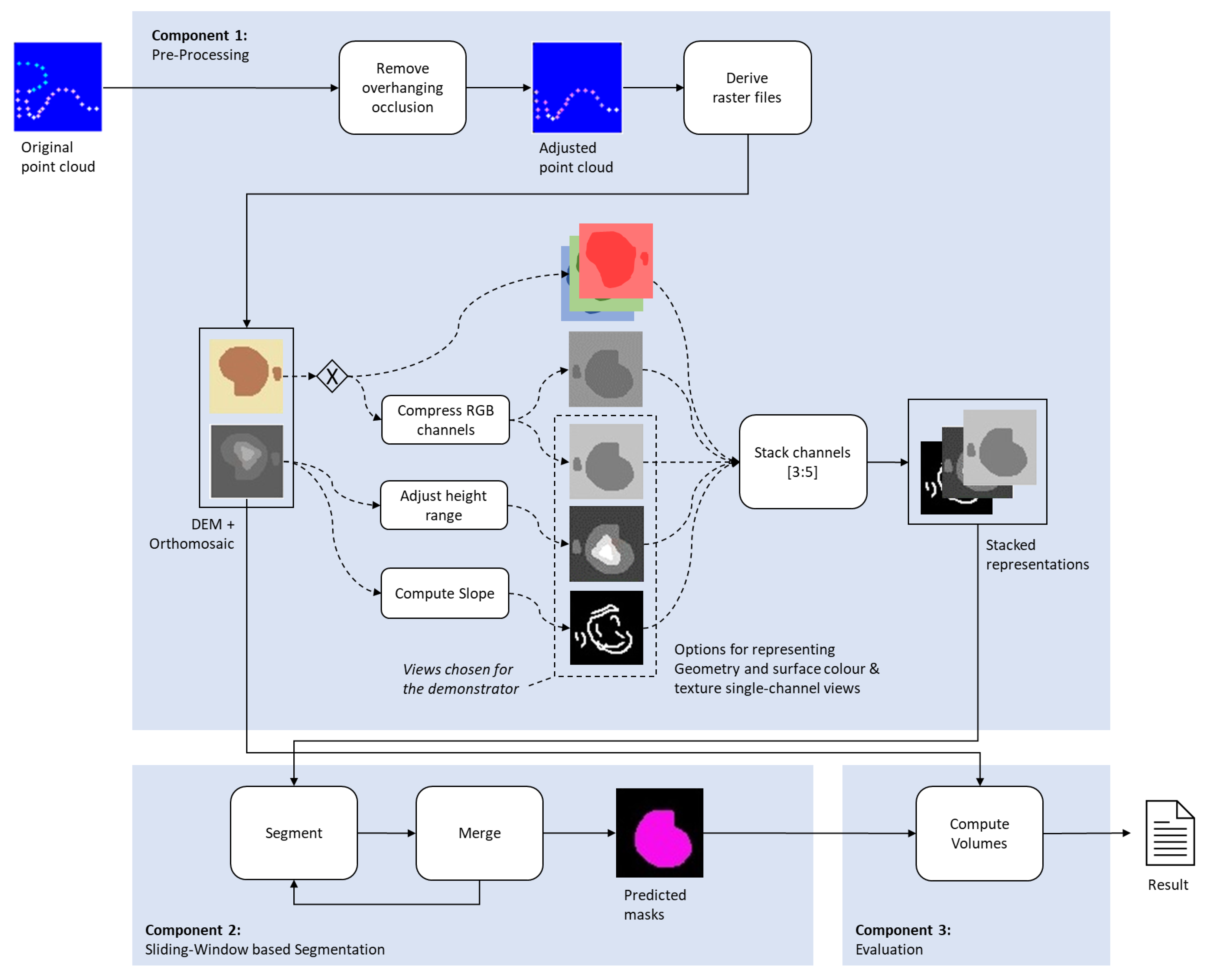
The stockpile segmentation approach proposed in this paper can be described as a pipeline of three components. The first component handles the necessary pre-processing steps. The first step of this component is to convert the 3D point cloud into a 2.5D raster format, creating the equivalent of a DEM and an Orthomosaic. This step is followed by optional feature transformation steps that compress information or highlight presumably valuable features. The final pre-processing step combines the resulting single channel views into a multi-channel input array. The second component performs the actual instance segmentation step using a sliding window-based approach. The third and final component computes the volumes per segmented stockpile based on the instance masks and the DEM.

Figure 6 illustrates this pipeline schematically. The small icons represent the data input and output of the individual processing steps. The first two blue icons show a sketch of a vertical cross-section through a 3D point cloud. The first scene shows a heap that stands next to a tree and partially under it. The second icon shows the same scene, but with all overhanging points removed. All following icons show the same scene, but as an idealized raster representation and from birds-eye view. Arrows with dashed lines symbolize alternative options for compressing and combining the information regarding color, height, and slope. Depending on the concrete implementation, different channels can be derived from the DEM and the Orthomosaic, and they can be combined in different ways (Note that not all the available combinations are sensible. The color information should either be provided using the original three-channel representation or a compressed representation, not both).

The combination chosen by the prototypical implementation of the demonstrator uses a greyscale view of the RGB image, an adjusted view of the heights and the pre-computed local slope (as is indicated by the dashed box around the respective channel icons) and combines them into a three-channel input array.

2.4. Component 1: Pre-Processing

2.4.1. Removing “Overhanging” Vertical Occlusions

The initial input of the pipeline proposed in this study is a three-dimensional RGB-point cloud which can be generated either via photogrammetry from overlapping aerial images or via LiDAR scan. An essential claim of this paper is that bulk material heaps themselves do not produce overhangs. Therefore their surface geometry can always be fully represented in the form of a digital elevation map.

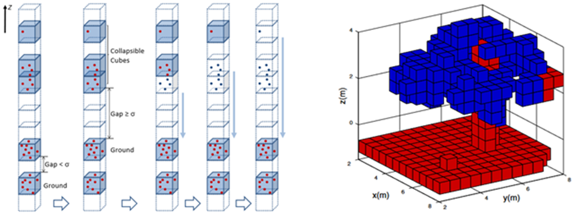
The goal of the first pre-processing step thus is to convert the 3D point cloud into a two-and-a-half-dimensional raster format that still fully represents the geometry and colors of all potential stockpile surfaces. To accomplish this, the first step is to remove all overhanging points by a rule-based algorithm that operates on a voxelized representation of the original point cloud. The algorithm is similar to a procedure called Collapsible Cubes proposed by [31]. The method divides the space occupied by the point cloud into a grid of regular cubes that are aligned with the local cartesian coordinate systems, commonly referred to as a voxel grid. Each vertical stack of cubes is traversed bottom to top. The first cube that contains points is considered as “ground”. If the next cube (the one on top) also contains points, those areas are also considered ground points. If, however, one or more cubes (the exact distance in terms of cubes is a parameter) that are empty follow a “ground” cube, any non-empty cubes above those are considered “overhang” (see Figure 7).

An expected limitation of this approach is the rare scenario where (1) bulk material is stored on top of an existing “overhanging” structure, like e.g., on top of a bridge, and (2) the ground under the bridge above which the bulk material is placed is sufficiently captured by the UAV-born surface scan. In most scenarios, however, this could be avoided by choosing flight path and sensor settings for the UAV in such a way that the ground beneath the bridge is not captured.

2.4.2. Converting the Adjusted Point Cloud to 2.5D Raster Format

Once all overhanging points are removed, the remaining points can be converted to (1) a true-color-orthomosaic and (2) a digital elevation model. This can be performed using e.g., the las2dem method [32] from the open source library and toolset LAStools [33]. This method converts a 3D point cloud in an intermediate step to a Triangulated Irregular Network [TIN] format and then creates a 2D raster representation from the TIN. The raster file can either contain information about RGB, elevation, slope, intensity, or various other information (if present in the original point cloud). Those raster files can subsequently be treated like regular image data.

This first component of the pipeline was not yet implemented in the current phase of the project and is thus only described theoretically in this paper. The results presented in [31], however, suggest that the described method provides a feasible solution. All subsequent components were implemented as described in Section 2.8. To test those components and to evaluate the result, the input for the second component was generated directly from a DEM and an Orthomosaic in TIFF file format. The respective surface scans of the test data contained almost no vertical occlusions, and thus the generated raster files served as a viable proxy for the expected output of component number one.

2.4.3. Compressing the RGB Color Information into Less than Three Channels (Optional)

To add geometrical features from the height map to the input array without changing the input channel dimension of the pre-trained model (compare Section 2.2.2), the original three-channel RGB orthomosaic must be compressed into less than three channels. There are several options to compress the RGB information:

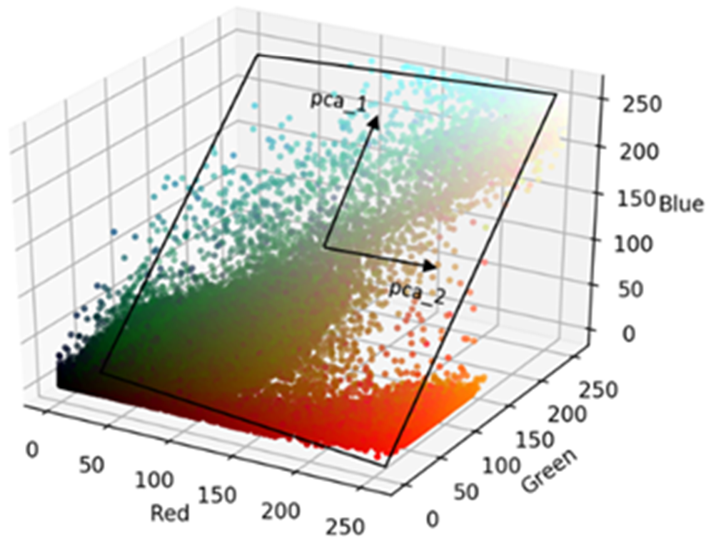
A simple method to compress all three channels into a single one is to compute a greyscale view as a weighted sum for each pixel over all three channels [34]. This method was chosen for the prototypical baseline implementation, which was used as a demonstrator in this study. An alternative approach is to convert the whole RGB image array into another color-space, e.g., Hue-Saturation-Value (HSV) [34], and then select one or two of the new channels to represent the color information. A third option is to utilize dimensionality reduction methods like Principal Component Analysis (PCA) [35] (p. 213–220) to project the information from a 3-dimensional color-space onto a lower-dimensional space, e.g., a 2-dimensional plane while minimizing information loss (see illustration in Figure 8).

A fourth option to reduce the amount of “space” to represent color information is known as color quantization [37]. In contrast to the methods above, this method would not reduce the dimensionality of the color information but rather its resolution. 8-bit color, for example, can encode 256 color values, including various shades of green, blue, red, magenta, orange, and yellow, while the subjective brightness varies from pure black to pure white. Evaluating which of the above-mentioned methods leads to the best results is subject to further research.

2.4.4. Increasing the Contrast of the Elevation Map (Optional)

The pixel values of the images in the COCO dataset on which the model was pretrained ranged from 0 to 255 for each channel. Therefore, the weights learned during pretraining were optimized to detect features in data of a similar range. In contrast to this, the relative height in the DEM usually only varies by less than thirty meters. To make the range of the new pixel values more similar to the range of the pixel values in the pretraining data, this preprocessing step “stretches” the relative heights in given DEM so that they range from 0 to 255. This is the equivalent of increasing the contrast of a greyscale image.

2.4.5. Computing the Local Slope (Optional)

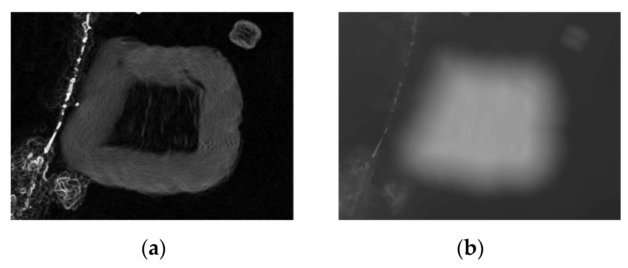
We propose a feature engineering step that computes the local slope and encodes it as a greyscale image (compare Figure 9). While a CNN, in principle, is able to figure out relevant patterns like a sudden change in slope given only a height map, the goal of this step is to help the model to perform better given the limited amount of domain-specific training data. Boundaries of objects in RGB images appear to be much more commonly indicated by sharp lines and/or sudden changes in brightness than by the beginning of a smooth transition from a darker to a brighter region. Therefore, the pre-trained model is more likely to infer object boundaries based on those features.

Pre-computing the slope as greyscale values is expected to enable the model to use basic contrast-related features learned during pre-training to infer heap boundaries, instead of having to figure out the local gradient of the height representation as a relevant feature for heap boundaries by itself.

2.4.6. Stacking the Individual Views

Once the three individual greyscale representations are created based on the original true color and elevation information, those 2D arrays are stacked along a third “channel-dimension” to create a new multi-channel array. For the prototypical implementation of the demonstrator we chose a combination of (1) a greyscale view of the RGB channels, (2) the height map with adjusted relative heights to increase the contrast, and (3) a greyscale representation of the local slope (see Figure 10).

2.5. Component 2: Sliding Window-Based Segmentation

2.5.1. Instance Segmentation Core

In contrast to semantic segmentation, which solely assigns a categorical label to each “atomic” element in the input data (e.g., a pixel in an image or a point in a point cloud), instance segmentation assigns two types of information: (1) the information to which class the element belongs and (2) the information to which individual object of this class the pixel belongs. This way, pixels that belong to the same object are directly grouped together.

Specialized model architectures exist to perform instance segmentation directly. In the case of 2D image instance segmentation, the model architecture Mask-RCNN [26] is reported to be among the best performing model architectures on large-scale open source datasets [38]. This model architecture was chosen as the segmentation algorithm for the current implementation of the proposed pipeline.

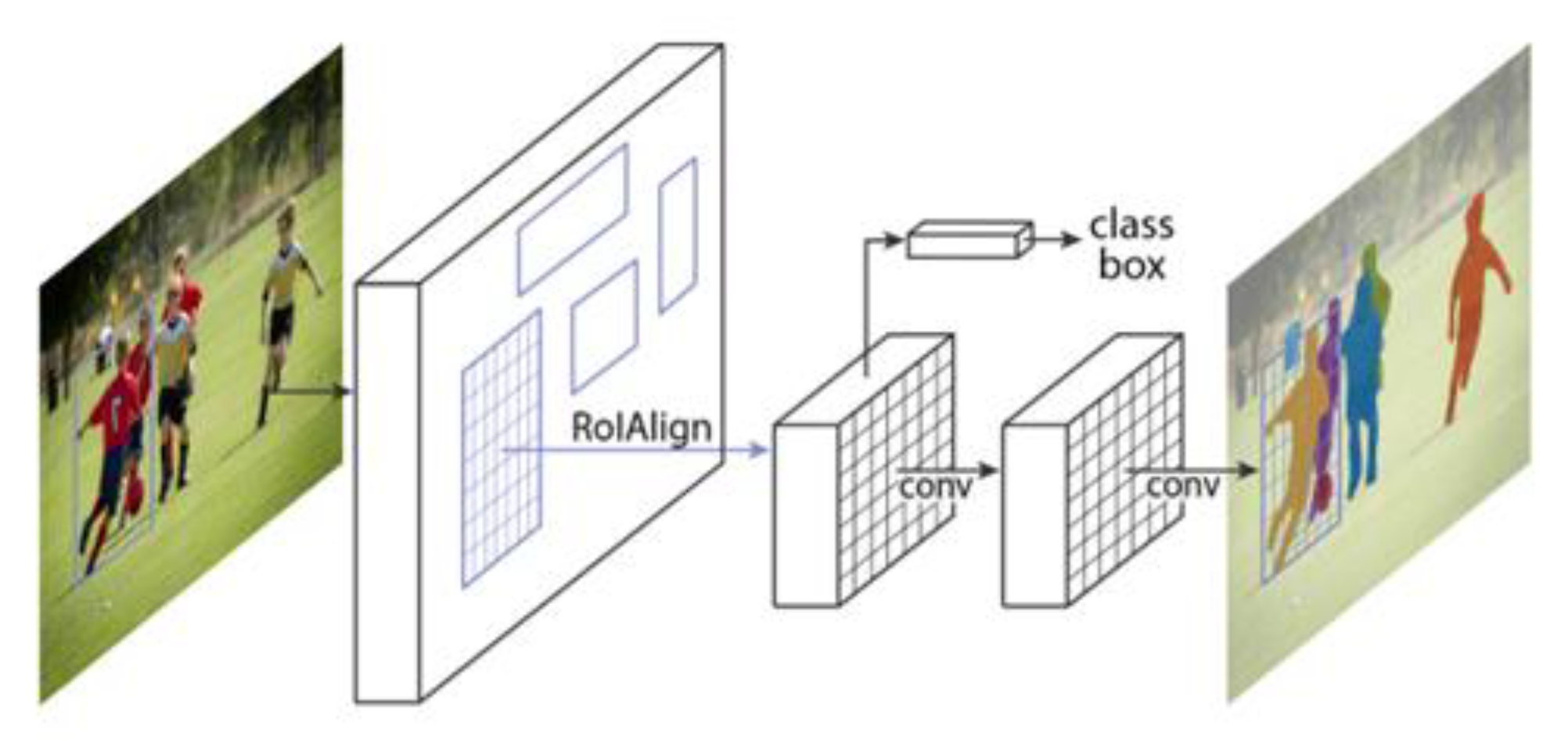
The Mask-RCNN model is based on top of Fast-RCNN [39] and consists of two main parts. The first part suggests rectangular regions of potential objects in the input image together with corresponding class scores for each region, and the second part performs a binary pixelwise segmentation in the suggested regions (see Figure 11).

While the Mask-RCNN architecture does not depend on a fixed input size (regarding the height and width of the input image), in practice there is still a limit regarding the maximum size of the input which the model can process in one go. This is mainly due to limitations regarding the available RAM (Random-Access-Memory) on the physical (or virtual) machine on which the algorithm runs.

2.5.2. Sliding Window-Based Processing of Large Sites

The method proposed in this paper addresses the issue of potentially very large input files using a sliding window-based approach to digest the input image in chunks (an input image, in this context, refers to the stacked views that were computed from the DEM and the orthomosaic, not to an actual single aerial photo). This way, the algorithm is no longer limited by the available RAM, but rather by the available disk size (since intermediate results can be stored on disk).

While this approach decouples the possible input size from the available RAM without having to sacrifice information due to, e.g., a reduction of the resolution, it creates another challenge—the instance-information is only valid within a single position of the sliding window. If the input image were simply cropped into individual tiles and then processed tile-by-tile, instances that span across two or more of those tiles would be cut into multiple independent objects. Figure 12 illustrates this problem, and the different color values represent distinct instance labels (also referred to as instance-indices). In the left sketch, instance labels are only valid within the individual tiles. To avoid this, a mechanism must be found to merge the instance-labels between adjacent positions of the sliding window in a meaningful way to produce a final result where “global” instance labels are valid across the entire scene, as illustrated in the right sketch in Figure 12.

The proposed approach addresses this problem by sliding the window in such a way that adjacent window positions overlap. The region where the two windows overlap thus gets segmented twice. Instances predicted in the two positions (hereafter also referred to as “tiles”) were then merged based on their spatial overlap in the “global” context of the large image. For each instance in “tile A”, the spatial overlap with each instance of “tile B” was computed. To quantify this overlap, the IoU score between the portion of instance n from Tile A that lies in the overlapping region and the portion of instance m from tile B that also lies in the overlapping region is computed. If the IoU score is larger than a given threshold, the two instances are “merged”, meaning they are both assigned the same global instance label. Figure 13 illustrates this concept.

An expected limitation of the sliding window-based approach is that the size of the largest heap that can be detected by this approach depends on the size of the sliding window. This is the case if a heap is of such a shape and size that part of its boundary cannot be detected by any of the of the sliding window positions. This problem, however, was not encountered for any of the heaps in the test set, where the largest heap was approximately 100 meters long and 30 meters wide (compare section “Preliminary Results”, the left-upper heap on test site B).

2.6. Component 3: Evaluation—Volume Computation

The enclosed volume per stockpile instance can be computed using the segmentation mask in combination with the DEM and, if available, a second DEM which represents the base ground on which the stockpile is located. Since the scale of the DEM is known, the area of represented surface per pixel is also known. The average height of the stockpile at each pixel is given by the respective height difference of the ground and the stockpile surface. Thus, the stockpile volume per pixel can be approximated as the volume of a column with a known base area and known height, and the total volume per stockpile can be calculated by summing the volumes of all pixels that lie inside the boundaries of a segmentation mask.

If the base surface is not available, the stockpile volume can only be estimated by making some assumptions about the shape of the stockpile’s base. Two possible options are (1) to interpolate the height of the borders of the stockpile, which is a good approximation for free-standing piles on relatively even grounds or (2) to assume a horizontal ground at the height of the lowest point of the stockpile boundary. The second assumption is more accurate if, e.g., a stockpile is piled up against a wall or in a box and rests on horizontal ground.

2.7. Evaluation Metrics

Two metrics are important to quantify the performance of an instance segmentation algorithm: (1) how well does the model perform on the object-level—how many objects are detected, missed, or falsely detected—and (2) how pixel-accurate is the segmentation among true-positive detections. Those metrics are coupled by the concept that defines whether an object as a whole is regarded as detected or not. For each individual object, the segmentation accuracy can be described using the Intersection-over-Union (IoU) score. This score is commonly used to evaluate the performance of semantic segmentation algorithms [40]. To measure the performance on the object level using precision and recall as metrics, it must first be defined what it means for a single object to be a “true-positive”. This can be done by setting a threshold for the IoU score on pixel level for each individual object. This method is commonly used to evaluate results in the context of object detection [41].

To evaluate the results of the proposed pipeline, an IoU threshold of > 0.5 was chosen since this value (a) seems to be the most intuitive of all arbitrary thresholds and (b) it is the lowest IoU score which each prediction can only share with a single ground-truth (and vice-versa). This value is also proposed in the context of panoptic segmentation by Kirillov et al. [42] for similar reasons.

The primary goal of the proposed stockpile segmentation pipeline is to allow for the automatic computation of the (approximated) volume per pile. Nevertheless, the central metric to describe the accuracy of the segmentation component was chosen to depend on the footprint area of the merged predictions, and not on the enclosed volumes, for the following reasons: (1) there is no fix relationship between the volumetric error and the footprint error, as this relationship depends on both the shape of the pile and on the “shape of the error” in relation to the pile’s true position, (2) the volumetric error can be small even though the footprint-error is large, since falsely detected areas can contain the same volume as the actual true area would have contained, and (3) the volumetric error is on average smaller than the footprint-error, thus evaluating the footprint-error gives a conservative performance estimate. The last point is due to the fact that the vast majority of pixelwise-segmentation errors occur in the outer region of a pile by segmenting either too much or too little, and not in the middle of a pile. The vast majority of stockpiles, on the other hand, are higher towards the middle and descend towards their borders. Therefore, a segmentation error on average has more impact on the IoU with regard to the footprint than on the actual volumetric error that follows from it (compare section “Preliminary Results”). However, this is only true on average, since there are segmentation errors and stockpile shapes that would lead to the opposite effect (see e.g., the sketch on the far right in Figure 14).

2.8. Prototype Implementation and Experimental Setup

A working prototype was implemented in python 3.8+ for components 2 to 4 of the proposed pipeline. The main libraries used are written in Python, C++, and CUDA. The main libraries and frameworks include the deep learning framework PyTorch [43], the computer vision library OpenCV [44], the scientific computing package NumPy [45], and the geospatial data translator library GDAL [46]. The segmentation component consists of a pretrained PyTorch implementation of the Mask-RCNN-architecture for instance-segmentation of image data. The weights were pretrained on the COCO dataset [30], which consist of 123,287 images, with a total of 886,284 instances from a large variety of classes.

The pipeline was developed and tested on an azure virtual machine of type Standard_NC6 [47]. The visualizations of the volumetric accuracy were created using the algorithmic modelling tool Grasshopper together with the 3D CAD program Rhino3D.

2.8.1. Pre-Processing

The implementation of the first two pre-processing steps, the removal of overhanging occlusions from the point cloud, and the creation of a DEM and a RGB-Orthomosaic from this point cloud, is pending. Suitable libraries for this component appear to be Open3D [48] for the voxel-based classification and removal of overhanging points and LAStools [33] for the creation of raster-files from the adjusted point cloud (compare Section 2.4.1).

The current implantation of the subsequent components directly imports the DEM and the respective Orthomosaic in TIFF file format. The DEM is transformed, cropped, and rescaled to the same location, coordinate system and context-size as the Orthomosaic using the python bindings for the GDAL library. The individual raster files are extracted as NumPy-arrays. The mapping of the actual height range to a range of 256 values, the derivation of the slope representation, and the stacking of the individual single-channel representations into one three-channel array was also performed using NumPy. The three-color channels are compressed into a single greyscale channel by computing an element-wise weighted sum across the original channels using OpenCV.

2.8.2. Model Training

The segmentation component uses a PyTorch implementation of the Mask-RCNN model with a ResNet-50 backbone with an additional Feature Pyramid Network (FPN). The model is loaded with weights pretrained on the COCO dataset. The box- and mask-predictor heads are replaced by new heads with only two output classes (“stockpile” and “background”).

The pre-trained model with the new model heads is trained on 7374 crops of a total of 15 individual training sites. Of the 5 blocks or the ResNet-50 backbone, blocks 1 and 2 were kept “frozen” during training on the domain-specific data, meaning their weights were not updated. The features used for the baseline model are height, slope and a greyscale view of the RGB Orthomosaic. The crops are generated with random positions and a randomly varied size between 500 × 500 and 1500x1500 pixel. The model was trained for 12 epochs using an initial learning rate of 1*e-4 and stepwise learning-rate decay with step-size = 5 and gamma = 0.1, meaning the learning rate is divided by a factor of 10 every 5 epochs. Training is stopped when the loss regarding the test set started to increase for three consecutive epochs. As an optimizer, a stochastic gradient descent (SGD) with momentum was chosen, with the momentum parameter set to 0.9. The only data augmentation performed on the fly during training was a random horizontal flip with a chance of 50%.

2.8.3. Inference

The sliding-window-based inference component of the pipeline uses a window size of 1000 × 1000 pixel with a stride of 400 pixel both vertically and horizontally. The ground-sample-distance of the input scene is 5cm per pixel, so the context size of each window is, on average, 50 × 50 meter. The IoU-threshold for merging instances within a single sliding window position (also referred to as “tile”) is set to 0.1, and the threshold for merging instances from two adjacent positions is set to 0.5. The minimum number of pixels per instance on tile-level is set to 5000, which would correspond to 12.5 square meters on the actual site.

The confidence thresholds on pixel and object levels are set to 0.5 and 0.05, respectively, based on the manual analysis of results for different values based on a small subset of the available test data. Regions above the object-threshold are considered predicted objects, and pixels above the respective threshold are considered as part of an object.

2.8.4. Volume Computation

The volume is computed as described in chapter 2.6 using an additional base DEM. The main libraries used were GDAL, Numpy, and OpenCV.

3. Preliminary Results

Preliminary results based on the working prototype and data from 15 training sites and 3 test sites demonstrate the general validity of the proposed method and pipeline. The results also offer a baseline for further feature combination and parameter optimization.

3.1. Footprint-Accuracy

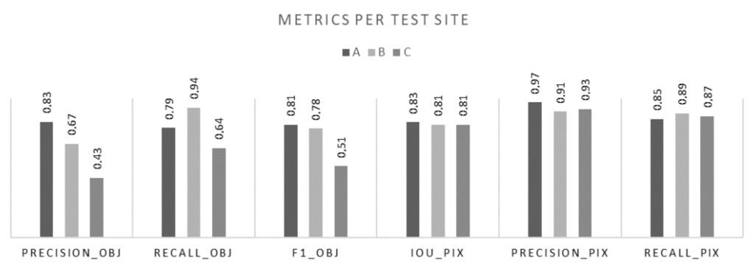
Figure 15 and

Table 1. Metrics per test site and average scores.

Test Site	Precision_Obj	Recall_Obj	F1_Obj	Iou_Pix	Precision_Pix	Recall_Pix	F1_Pix
A	0.83	0.79	0.81	0.83	0.97	0.85	0.91
B	0.67	0.94	0.78	0.81	0.91	0.89	0.90
C	0.43	0.64	0.51	0.81	0.93	0.87	0.90
Average	0.65	0.79	0.70	0.82	0.93	0.87	0.90

show the test-scores with regards to test sites A, B and C. On the object-level, the average precision across the three test sites was 0.65 and the average recall was 0.79, which results in an F1-score of 0.7. The average IoU among true-positives was 0.82, the average precision on the pixel-level was 0.93, and the average recall on the pixel-level was 0.87. This results in an F1-score on pixel level of 0.90. All results were computed using the IoU-threshold of >0.5 for true-positives (as discussed in the previous section).

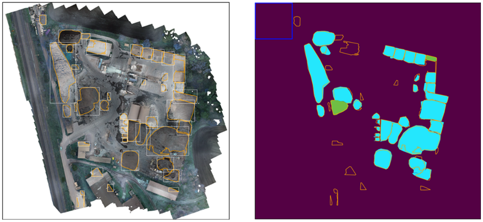
Figure 16, Figure 17 and Figure 18 present the prediction result visually. The left image shows an RGB orthomosaic of the scene with the prediction boundaries plotted on top. The orange polygons denote the boundaries of the pixel masks per instance, and the white bounding boxes highlight the individual instances. The right image plots the predictions on top of the ground truth masks. The color of the individual GT masks denotes whether a GT instance was considered to be detected on the object-level: blue masks denote true-positives, green masks denote false negatives. Orange boundary polygons with none or insufficient overlap with GT masks show false positives. The orange polygons in general denote the boundaries of the predicted pixel masks the same way as they do in the left image. The blue square in the top-left corner of the right image illustrates the size of the sliding window in context.

3.2. Volumetric Accuracy

As stated in Section 2.7, it is assumed that the volumetric accuracy is, on average, greater than the footprint accuracy. This assumption was tested using a subset of 17 piles from test site A by assessing both the IoU score and the volumetric accuracy of the predictions. The volumetric analysis was limited to piles from test site A since it was the only one with a base DEM available, and therefore the only one that allowed for accurate volume computation without introducing inaccuracies in the result-evaluation itself due to simplified ground level assumptions. To quantify the volumetric accuracy, the smaller volume of both prediction and ground-truth per pile was divided by the larger volume. The volume accuracy thus ranges from 0.0 to 1.0. To quantify the footprint-accuracy, the standard IoU measurement was chosen.

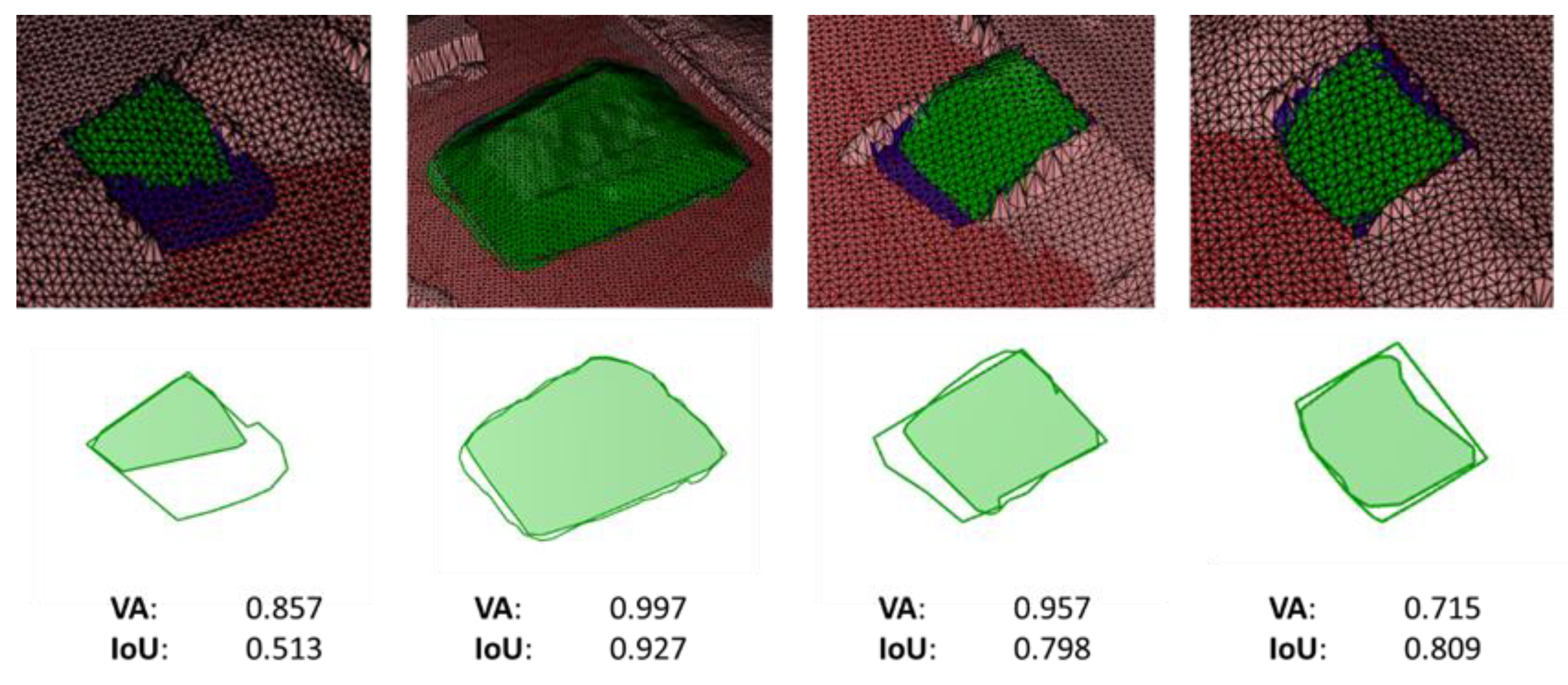
On average, the IoU score with regard to the footprints was 0.85, while the average volumetric accuracy was 0.92.

Table 2. IoU-scores regarding the footprint-areas and volumetric accuracy regarding the true and the predicted volume. The table shows the results for 17 true-positive predictions from test site A as well as the average results across all 17 piles.

Pile	1	2	3	4	5	6	7	8	9	10	11	12	13	14	15	16	17	AVG
area IoU	0.91	0.84	0.97	0.92	0.80	0.90	0.83	0.92	0.84	0.89	0.82	0.51	0.80	0.92	0.83	0.78	0.85	0.85
Volume Accuracy	0.99	0.90	0.99	0.96	0.71	0.91	0.95	0.97	0.87	0.90	0.81	0.86	0.96	0.99	0.81	0.82	0.93	0.92

shows this comparison based on 17 heaps, and Figure 19 shows four exemplary heaps to illustrate the relationship between volumetric error and footprint-error. In the 3D mesh view, the ground-truth surface area is marked purple, and the predicted area is marked green. The surface areas where prediction and ground truth overlap are also marked green. In the 2D footprint view below those images, the intersection area is marked solid green, and the false-positive and false-negative area is marked white with a green line as border.

For heap number one and three (left to right), the error consists largely of false-negative areas in the lower parts of the heaps. Since there is relatively little material in these areas, they contribute little to the overall volume, therefore the footprint-IoU is more affected by this error than the volumetric accuracy. In the case of heap number 2 (second from the left), the predicted heap is slightly larger than the actual heap. Since this false-positive area falls completely on the flat surrounding ground, it has almost no effect on the volumetric accuracy. The example on the far right shows a pile in a box where the larger part of the foot-print error falls in the region where the pile is the tallest. In this case, the error has a larger effect on the volumetric accuracy than on the footprint-IoU.

4. Discussion

The initial claim of this paper was that the proposed solution was able to detect and segment various types of piles in various surroundings. Concretely, it was stated that the method allows for (1) the segmentation of heaps with “atypical” shapes, (2) the segmentation of heaps that stand on a surface made of the same material as the heap itself, (3) segment individual heaps of the same material type that border each other, and (4) differentiate between artificial heaps and other objects of similar shape like natural hills.

Figure 20 zooms in on an area from test site B that supports claim number (1). Here, different types of piles are segmented with relative high accuracy. The area includes 4 piles in boxes, 1 pile in a corner, 1 pile piled up against a wall, 1 (mostly) free standing pile, and 2 piles of very similar (but possibly not identical) material that border each other.

Figure 21 supports claim number (2): the ability to segment individual piles that border each other and consist of the same material. It also partially supports claim number (3): the ability to segment piles that stand on ground covered with the same material that constitutes the pile. Not the entire area that is covered with this material is classified as part of a stockpile, which displays the ability of the model to distinguish between bulk material in general and bulk material heaps. However, in the given example, it is ambiguous as to what a “perfect” segmentation would look like and if not classifying parts of the area was a correct decision in this specific case.

Figure 22 is presented as an example with regard to claim number 4—the claim that the approach is able to distinguish between bulk material heaps and hills that are part of the landscape. The results in that regard are inconclusive, since there was only one hill present at the test set. Although most of this hill was correctly ignored, a small part of it was falsely marked as “heap”.

4.1. Error Analysis

4.1.1. False Positives

On average, the precision is lower than the recall (compare Figure 15). On test site A and B, most of the false positives come from relatively small objects close to the edge of the respective sliding window position. It stands to reason that this is because at the outer regions of the sliding window, there is relatively little context for any given pixel, compared to regions in the middle of the window. It is unknown how parts of potential objects in this region continue outside the current frame, which makes it more likely to misinterpret objects in those regions.

However, this effect only produces false positives and not false negatives since a false-positive must only be predicted once, whilst a false negative in most cases must be produced multiple times for the same region. This is due to the way the sliding window traverses the site with a stride of 0.4. All parts of the site, except for the outer most 400 pixels, are seen multiple times. A region that was part of the border region of one sliding window position lies close to the center when the window is at the right or lower adjacent position.

A possible solution to reduce the number of false positives due to this effect could be to only consider predictions that reach into a pre-defined inner region of the sliding window. The distance of this inner region to the window’s borders would constitute another hyperparameter during inference. The effect of such a mechanism, together with suitable values for the respective distance-parameter, is subject to further research.

Other common types of errors were (1) piles of crushed metal on a scrapyard neighboring test site C, (2) parts of roofs (compare Figure 23, panels b to c), and (3) flat surface areas that, on the RGB orthomosaic, resembled stockpiles. On test site C, 4 out of 19 false positives come from heaps of crushed metal in a neighboring scrapyard. On test site B, 5 out of 13 false positives occurred due to the model confusing parts of roofs with stockpiles.

4.1.2. False Negatives

One of the main reasons for false negatives was falsely merging two or more instances together (see Figure 24). This reason accounts for 2 out of 2 false negatives on site B and 5 out of 9 false positives on site C. The merged prediction itself was additionally counted as false positive. The remaining false positives, including all 4 from test-site A, are either due to a confidence value on the object level that was below the threshold or a predicted region on the pixel level that had an IoU score below 0.5 with the GT.

4.2. Semi-Automated Inventory System and Human-in-the-Loop

While the results demonstrate the general feasibility of the proposed method, the accuracy produced on the three test sites given the 15 training sites and the current set of features and hyperparameters appears to be insufficient for the use in a fully automatic inventory system. However, performance is expected to improve with more training data and optimized feature and parameter settings.

However, the current pipeline could be utilized in a semi-automated fashion, where the results are validated—and adjusted, if necessary—by a human supervisor before the final report is created. The system could be designed to support a human-in-the-loop workflow, where corrections made by the human supervisor are periodically used to retrain the segmentation algorithm, thus enabling the system to “learn from its mistakes”.

4.3. Outlook and Further Research

The preliminary results presented above were produced by a pipeline that used a fixed set of features and hyperparameters. Chosen features were (1) a greyscale view of the RGB orthomosaic computed as an element-wise weighted sum across the original color channels, (2) the adjusted relative heights, and (3) the slope derived from the high-resolution DEM. The parameters of the sliding window component were set to a context-size of 50 × 50 meters and a stride of 40%. The results from this setting serve as a baseline for further experiments.

A comprehensive and systematic evaluation of the influence of different feature representations and hyper-parameter settings is the primary subject of further research. Preliminary results based on a small set of 600 training tiles used for fast experimentation suggest that a model which has access to both color and geometry features performs better than models that have access to only one of those feature types.

Figure 25 shows an example where a model trained solely on relative heights (represented as RGB heat map) detects only one of two heaps in the image. A model which has access to only true-color RGB values detected none of the heaps. A third mode, which used the relative height together with the original blue and green channel, was able to detect both heaps quite accurately. Those results, however, merely show qualitative effects. A quantitative analysis using the methods and metrics described in this article is pending.

Other topics of further research are (1) the mechanism proposed in Section 4.1.1, which aims to reduce the number of false positives by only taking into account predictions that reach into a pre-defined inner region of each sliding window position and (2) the implementation and evaluation of component number 1, which removes overhanging vertical occlusions from a 3D RGB point cloud and converts the remaining points into a 2.5D raster grid representation.

Finally, the current approach, which reduces the dimensionality of the color information in order to feed additional geometric information to a pretrained model implementation with 3 input channels, is to be compared to an adjusted model implementation that supports more than three input channels.

5. Conclusions

This paper proposed a novel method to segment instances of bulk material heaps from UAV-born aerial data using a pretrained CNN for instance-segmentation and information about the surface color, texture, and topography represented in raster-grid format as input features.

The method was validated by a working prototype and tested on three previously unseen material handling sites that contained a total of 77 individual bulk material heaps. The method achieved an average object detection precision of 0.65 and a recall of 0.79. The average IoU-score on pixel-level regarding the predicted footprint-areas across all predictions that are regarded as “true-positives” is 0.82. The volumetric accuracy, which was determined on a subset of the predicted heaps, was 0.92 on average larger than the footprint-IoU-score (which was 0.85 for the same subset of heaps).

Those results present a baseline for further optimization regarding feature transformations and combinations, as well as the tuning of pipeline-specific hyperparameters like the context-size, the stride of the sliding window, and confidence thresholds regarding both object- and pixel-level. A systematic evaluation of those options is subject to further research.

Additionally, a pre-processing step was proposed, which removes all overhanging vertical occlusions from a 3D point cloud and converts the remaining points into a 2.5D raster format. This step follows from the assumption that bulk material itself will never produce overhangs and thus the lowest surface in a 3D surface scan constitutes the bulk material surface. Exceptions to this assumption are sites where the bulk material is stored on top of overhanging structures, such as on top of a bridge.

References

1. Tucci, G.; Gebbia, A.; Conti, A.; Fiorini, L.; Lubello, C. Monitoring and Computation of the Volumes of Stockpiles of Bulk Material by Means of UAV Photogrammetric Surveying. Remote Sens. 2019, 11, 1471. [Google Scholar] [CrossRef] [Green Version]
2. Thomas, H.R.; Riley, D.R.; Messner, J.I. Fundamental Principles of Site Material Management. J. Constr. Eng. Manag. 2005, 131, 808–815. [Google Scholar] [CrossRef]
3. Agboola, O.; Babatunde, D.E.; Fayomi, O.S.I.; Sadiku, E.R.; Popoola, P.; Moropeng, L.; Yahaya, A.; Mamudu, O.A. A review on the impact of mining operation: Monitoring, assessment and management. Results Eng. 2020, 8, 100181. [Google Scholar] [CrossRef]
4. Kovanič, L.; Blistan, P.; Štroner, M.; Urban, R.; Blistanova, M. Suitability of Aerial Photogrammetry for Dump Documentation and Volume Determination in Large Areas. Appl. Sci. 2021, 11, 6564. [Google Scholar] [CrossRef]
5. Yang, X.; Huang, Y.; Zhang, Q. Automatic Stockpile Extraction and Measurement Using 3D Point Cloud and Multi-Scale Directional Curvature. Remote Sens. 2020, 12, 960. [Google Scholar] [CrossRef] [Green Version]
6. Son, S.W.; Kim, D.W.; Sung, W.G.; Yu, J.J. Integrating UAV and TLS Approaches for Environmental Management: A Case Study of a Waste Stockpile Area. Remote Sens. 2020, 12, 1615. [Google Scholar] [CrossRef]
7. Liu, J.; Liu, X.; Lv, X.; Wang, B.; Lian, X. Novel Method for Monitoring Mining Subsidence Featuring Co-Registration of UAV LiDAR Data and Photogrammetry. Appl. Sci. 2022, 12, 9374. [Google Scholar] [CrossRef]
8. Godone, D.; Allasia, P.; Borrelli, L.; Gullà, G. UAV and Structure from Motion Approach to Monitor the Maierato Landslide Evolution. Remote Sens. 2020, 12, 1039. [Google Scholar] [CrossRef] [Green Version]
9. Park, H.C.; Rachmawati, T.S.N.; Kim, S. UAV-Based High-Rise Buildings Earthwork Monitoring—A Case Study. Sustainability 2022, 14, 10179. [Google Scholar] [CrossRef]
10. Carabassa, V.; Montero, P.; Alcañiz, J.M.; Padró, J.-C. Soil Erosion Monitoring in Quarry Restoration Using Drones. Minerals 2021, 11, 949. [Google Scholar] [CrossRef]
11. A Ab Rahman, A.; Maulud, K.N.A.; A Mohd, F.; Jaafar, O.; Tahar, K.N. Volumetric calculation using low cost unmanned aerial vehicle (UAV) approach. IOP Conf. Ser. Mater. Sci. Eng. 2017, 270, 012032. [Google Scholar] [CrossRef] [Green Version]
12. Alsayed, A.; Yunusa-Kaltungo, A.; Quinn, M.K.; Arvin, F.; Nabawy, M.R.A. Drone-Assisted Confined Space Inspection and Stockpile Volume Estimation. Remote Sens. 2021, 13, 3356. [Google Scholar] [CrossRef]
13. Jiang, Y.; Huang, Y.; Liu, J.; Li, D.; Li, S.; Nie, W.; Chung, I.-H. Automatic Volume Calculation and Mapping of Construction and Demolition Debris Using Drones, Deep Learning, and GIS. Drones 2022, 6, 279. [Google Scholar] [CrossRef]
14. Sivitskis, A.J.; Lehner, J.W.; Harrower, M.J.; Dumitru, I.A.; Paulsen, P.E.; Nathan, S.; Viete, D.R.; Al-Jabri, S.; Helwing, B.; Wiig, F.; et al. Detecting and Mapping Slag Heaps at Ancient Copper Production Sites in Oman. Remote Sens. 2019, 11, 3014. [Google Scholar] [CrossRef] [Green Version]
15. Finkbeiner, M.S.; Uchiyama, N.; Sawodny, O. Shape Recognition of Material Heaps in Outdoor Environments and Optimal Excavation Planning. In Proceedings of the 2019 International Electronics Symposium (IES), Surabaya, Indonesia, 27–28 September 2019; pp. 58–62. [Google Scholar] [CrossRef]
16. Canny, J. A Computational Approach to Edge Detection. IEEE Trans. Pattern Anal. Mach. Intell. 1986, 8, 679–698. [Google Scholar] [CrossRef]
17. Kumar, C.; Mathur, Y.; Jannesari, A. Efficient Volume Estimation for Dynamic Environments using Deep Learning on the Edge. In Proceedings of the 2022 IEEE International Parallel and Distributed Processing Symposium Workshops (IPDPSW), Lyon, France, 30 May–3 June 2022; pp. 995–1002. [Google Scholar] [CrossRef]
18. Fan, H.; Tian, Z.; Xu, X.; Sun, X.; Ma, Y.; Liu, H.; Lu, H. Rockfill material segmentation and gradation calculation based on deep learning. Case Stud. Constr. Mater. 2022, 17, e01216. [Google Scholar] [CrossRef]
19. Huang, H.; University of Illinois Urbana-Champaign; Tutumluer, E.; Luo, J.; Ding, K.; Qamhia, I.; Hart, J. 3D Image Analysis Using Deep Learning for Size and Shape Characterization of Stockpile Riprap Aggregates—Phase 2; Illinois Center for Transportation: Rantoul, IL, USA, 2022. [Google Scholar] [CrossRef]
20. Hyde, D.; Raffman, D. Sorites Paradox. In The Stanford Encyclopedia of Philosophy; Zalta, E.N., Ed.; Metaphysics Research Lab, Stanford University: Stanford, CA, USA, 2018; Available online: https://plato.stanford.edu/archives/sum2018/entries/sorites-paradox/ (accessed on 25 October 2022).
21. Kaijaluoto, R.; Kukko, A.; El Issaoui, A.; Hyyppä, J.; Kaartinen, H. Semantic segmentation of point cloud data using raw laser scanner measurements and deep neural networks. ISPRS Open J. Photogramm. Remote Sens. 2022, 3, 100011. [Google Scholar] [CrossRef]
22. Qi, C.R.; Su, H.; Mo, K.; Guibas, L.J. PointNet: Deep Learning on Point Sets for 3D Classification and Segmentation. In Proceedings of the IEEE Conference on Computer Vision and Pattern Recognition, Honolulu, HI, USA, 21–26 July 2017; pp. 652–660. Available online: https://openaccess.thecvf.com/content_cvpr_2017/html/Qi_PointNet_Deep_Learning_CVPR_2017_paper.html (accessed on 22 October 2022).
23. Zhao, H.; Jiang, L.; Fu, C.-W.; Jia, J. PointWeb: Enhancing Local Neighborhood Features for Point Cloud Processing. In Proceedings of the IEEE/CVF Conference on Computer Vision and Pattern Recognition (CVPR), Long Beach, CA, USA, 15–20 June 2019; pp. 5560–5568. [Google Scholar] [CrossRef]
24. Cui, Y.; Chen, R.; Chu, W.; Chen, L.; Tian, D.; Li, Y.; Cao, D. Deep Learning for Image and Point Cloud Fusion in Autonomous Driving: A Review. IEEE Trans. Intell. Transp. Syst. 2022, 23, 722–739. [Google Scholar] [CrossRef]
25. Griffiths, D.; Boehm, J. A Review on Deep Learning Techniques for 3D Sensed Data Classification. Remote Sens. 2019, 11, 1499. [Google Scholar] [CrossRef] [Green Version]
26. He, K.; Gkioxari, G.; Dollár, P.; Girshick, R. Mask R-CNN. In Proceedings of the IEEE International Conference on Computer Vision, Venice, Italy, 22–29 October 2017. [Google Scholar] [CrossRef]
27. Zhuang, F.; Qi, Z.; Duan, K.; Xi, D.; Zhu, Y.; Zhu, H.; Xiong, H.; He, Q. A Comprehensive Survey on Transfer Learning. Proc. IEEE 2021, 109, 43–76. [Google Scholar] [CrossRef]
28. Kentsch, S.; Caceres, M.L.L.; Serrano, D.; Roure, F.; Diez, Y. Computer Vision and Deep Learning Techniques for the Analysis of Drone-Acquired Forest Images, a Transfer Learning Study. Remote Sens. 2020, 12, 1287. [Google Scholar] [CrossRef] [Green Version]
29. Maqsood, M.; Nazir, F.; Khan, U.; Aadil, F.; Jamal, H.; Mehmood, I.; Song, O.-Y. Transfer Learning Assisted Classification and Detection of Alzheimer’s Disease Stages Using 3D MRI Scans. Sensors 2019, 19, 2645. [Google Scholar] [CrossRef] [PubMed] [Green Version]
30. COCO—Common Objects in Context. Available online: https://cocodataset.org/#explore (accessed on 19 October 2022).
31. Reina, A.J.; Martínez, J.L.; Mandow, A.; Morales, J.; García-Cerezo, A.; Martínez, J.L.; Morales, J. Collapsible cubes: Removing overhangs from 3D point clouds to build local navigable elevation maps. In Proceedings of the 2014 IEEE/ASME International Conference on Advanced Intelligent Mechatronics, Besançon, France, 8–11 July 2014; pp. 1012–1017. [Google Scholar] [CrossRef]
32. las2dem_README. Available online: http://www.cs.unc.edu/~isenburg/lastools/download/las2dem_README.txt (accessed on 14 October 2022).
33. LAStools. 12 October 2022. Available online: https://github.com/LAStools/LAStools (accessed on 14 October 2022).
34. OpenCV: Color Conversions. Available online: https://docs.opencv.org/3.4/de/d25/imgproc_color_conversions.html (accessed on 17 October 2022).
35. Géron, A. Hands-On Machine Learning with Scikit-Learn, Keras, and TensorFlow: Concepts, Tools, and Techniques to Build Intelligent Systems, 2nd ed.; O’Reilly Media, Inc.: Sebastopol, CA, USA, 2019. [Google Scholar]
36. Python, R. Image Segmentation Using Color Spaces in OpenCV + Python–Real Python. Available online: https://realpython.com/python-opencv-color-spaces/ (accessed on 17 October 2022).
37. Color Quantization Using K-Means. Scikit-Learn. Available online: https://scikit-learn/stable/auto_examples/cluster/plot_color_quantization.html (accessed on 22 October 2022).
38. Minaee, S.; Boykov, Y.Y.; Porikli, F.; Plaza, A.J.; Kehtarnavaz, N.; Terzopoulos, D. Image Segmentation Using Deep Learning: A Survey. IEEE Trans. Pattern Anal. Mach. Intell. 2022, 44, 3523–3542. [Google Scholar] [CrossRef] [PubMed]
39. Girshick, R. Fast R-CNN. In Proceedings of the IEEE International Conference on Computer Vision, Santiago, Chile, 7–13 December 2015; pp. 1440–1448. Available online: https://openaccess.thecvf.com/content_iccv_2015/html/Girshick_Fast_R-CNN_ICCV_2015_paper.html (accessed on 22 October 2022).
40. Thoma, M. A Survey of Semantic Segmentation. arXiv 2016, arXiv:1602.06541. [Google Scholar]
41. Padilla, R.; Netto, S.L.; da Silva, E.A.B. A Survey on Performance Metrics for Object-Detection Algorithms. In Proceedings of the 2020 International Conference on Systems, Signals and Image Processing (IWSSIP), Niteroi, Brazil, 1–3 July 2020; pp. 237–242. [Google Scholar]
42. Kirillov, A.; He, K.; Girshick, R.; Rother, C.; Dollar, P. Panoptic Segmentation. In Proceedings of the IEEE/CVF Conference on Computer Vision and Pattern Recognition, Long Beach, CA, USA, 16–20 June 2019; pp. 9404–9413. Available online: https://openaccess.thecvf.com/content_CVPR_2019/html/Kirillov_Panoptic_Segmentation_CVPR_2019_paper.html (accessed on 17 October 2022).
43. PyTorch. Available online: https://www.pytorch.org (accessed on 26 October 2022).
44. OpenCV. Available online: https://opencv.org/ (accessed on 26 October 2022).
45. NumPy. Available online: https://numpy.org/ (accessed on 15 October 2022).
46. GDAL-Geospatial Data Abstraction Library. Open Source Geospatial Foundation, 26 October 2022. Available online: https://github.com/OSGeo/gdal (accessed on 26 October 2022).
47. Azure VM Comparison. Available online: https://azureprice.net/vm/Standard_NC6 (accessed on 21 October 2022).
48. Open3D: A Modern Library for 3D Data Processing—Open3D 0.15.1 Documentation. Available online: http://www.open3d.org/docs/release/ (accessed on 15 October 2022).
Figure 1. Point clouds of two construction material industry sites.
Remotesensing 15 00211 g001
Figure 2. Context and industrial application of material heap recognition.
Remotesensing 15 00211 g002
Figure 3. Semantic segmentation of regions that contain demolition debris [13].
Remotesensing 15 00211 g003
Figure 4. Stockpile extraction from point clouds based on bi-directional curvature [5].
Remotesensing 15 00211 g004
Figure 5. Segmentation of individual grains in bulk material. (left) from 2D images [18], (right) from 3D point cloud [19].
Remotesensing 15 00211 g005
Figure 6. Proposed pipeline; schematic.
Remotesensing 15 00211 g006
Figure 7. Illustration of the “Collapsible Cubes” procedure to identify “ground” and “non-ground” points [31].
Remotesensing 15 00211 g007
Figure 8. Illustration of a plane spanned by the first two principal component vectors of a color-point-distribution in 3D RGB-Space, based on [36].
Remotesensing 15 00211 g008
Figure 9. A heap shown (a) in “slope-view” and (b) in “height-view”.
Remotesensing 15 00211 g009
Figure 10. Aerial data of a stockpile site represented as (a) RGB orthomosaic as greyscale, (b) adjusted relative heights as greyscale, (c) local gradient, and (d) all three views stacked vertically along the channel dimension and displayed as RGB false color.
Remotesensing 15 00211 g010
Figure 11. Illustration of the Mask-RCNN principal for instance segmentation [26].
Remotesensing 15 00211 g011
Figure 12. Local instance labels per tile (a) vs. global instance labels of merge result (b).
Remotesensing 15 00211 g012
Figure 13. Merging of instances between adjacent sliding widow positions.
Remotesensing 15 00211 g013
Figure 14. Relationship between segmentation errors regarding footprint and volume for different error types and pile shapes; illustration.
Remotesensing 15 00211 g014
Figure 15. Metrics per test site.
Remotesensing 15 00211 g015
Figure 16. Results on Test Site A. (a) Boundary polygons (orange) and bounding boxes (white) plotted on top of the RGB orthomosaic; (b) Boundary polygons plotted on top of the ground truth masks. Light-blue masks denote true positives, green masks denote false negatives. The blue square in the upper-left corner illustrates the size of a single sliding window position in relation to the size of the whole site.
Remotesensing 15 00211 g016
Figure 17. Results on Test Site B. Colors and shapes have the same meaning as on test site A.
Remotesensing 15 00211 g017
Figure 18. Results on Test Site C. Colors and shapes have the same meaning as on test site A.
Remotesensing 15 00211 g018
Figure 19. Prediction and ground truth projected on the surface scan (as mesh).
Remotesensing 15 00211 g019
Figure 20. Selected area from test site B as an example for the accurate detection and segmentation of different types of piles. Displayed (a) as RGB orthomosaic, (b) as relative heights, (c) as local slope, and (d) as RGB orthomosaic, together with the predictions as polygon-boundaries and bounding boxes.
Remotesensing 15 00211 g020
Figure 21. Selected area from test site B as an example for the correct segmentation of individual piles that consist of the same material and border each other.
Remotesensing 15 00211 g021
Figure 22. Selected area from test site A as an example for the ability to distinguish between bulk material heaps and hills that are part of the landscape.
Remotesensing 15 00211 g022
Figure 23. Frequent types of false positives. (a) small predictions at the outer region of the sliding window; (b) piles of crushed metal from a neighboring scrapyard; (c) edges of roofs.
Remotesensing 15 00211 g023
Figure 24. False negatives due to incorrect merging of multiple instances into a single instance.
Remotesensing 15 00211 g024
Figure 25. Results from different models using different feature combinations shown for the same area of test site B. (a) One out of two heaps detected by a model using only relative height represented as RGB heat map as features. (b) None of the two heaps were detected by a model using the RGB true color of the orthomosaic as features. (c) Both heaps accurately detected by a model that uses relative height together with the green and the blue channel as features. (d) The respective ground-truth masks.
Remotesensing 15 00211 g025