TSRC: A Deep Learning Model for Precipitation Short-Term Forecasting over China Using Radar Echo Data

Abstract

Currently, most deep learning (DL)-based models for precipitation forecasting face two conspicuous issues: the smoothing effect in the precipitation field and the degenerate effect of forecasting precipitation intensity. Therefore, this study proposes “time series residual convolution (TSRC)”, a DL-based convolutional neural network for precipitation nowcasting over China with a lead time of 3 h. The core idea of TSRC is it compensates the current local cues with previous local cues during convolution processes, so more contextual information and less uncertain features would remain in deep networks. We use four years’ radar echo reflectivity data from 2017 to 2020 for model training and one year’s data from 2021 for model testing and compare it with two commonly used nowcasting models: optical flow model (OF) and UNet. Results show that TSRC obtains better forecasting performances than OF and UNet with a relatively high probability of detection (POD), low false alarm rate (FAR), small mean absolute error (MAE) and high structural similarity index (SSIM), especially at longer lead times. Meanwhile, the results of two case studies suggest that TSRC still introduces smoothing effects and slightly outperforms UNet at longer lead times. The most considerable result is that our model can forecast high-intensity radar echoes even for typhoon rainfall systems, suggesting that the degenerate effect of forecasting precipitation intensity can be improved by our model. Future works will focus on the combination of multi-source data and the design of the model’s architecture to gain further improvements in precipitation short-term forecasting.

1. Introduction

While precipitation brings convenience to agricultural production and lives, it also increases the risk of natural disasters. Accurate precipitation forecast, as an important branch in weather forecast, is a prerequisite for policy-making, risk management and the reduction of loss of life and property. Therefore, it has received intensive research in the hydrometeorological community. However, real-time, large-scale and fine-grid precipitation forecast, especially nowcast (0–2 h) or short-term forecast (0–6 h), remains greatly challenging due to the inherent complexities of the dynamics of the atmosphere [1].

Existing models for precipitation forecast mainly fall into two types: numerical weather prediction-based (NWP) models [2,3,4] and extrapolation models based on radar echoes and satellite observations [5,6,7]. NWP models release predictions by describing hydrodynamical and thermodynamical equations with the atmosphere’s initial and boundary conditions. However, NWP models struggle to capture convective scale patterns that occur in mesoscale systems because computational restrictions limit the fine-resolution configurations and spin-up times [2,8,9]. Therefore, NWP models are still inefficient in modeling cloud dynamics and microphysics, so precipitation nowcasts and short-term forecasts are arguably invalid [10,11,12]. Extrapolation models are mainly based on the advection of present cloud motional features and trajectories and then reckon future shapes, locations and intensities of precipitation field at a lead time of a few hours. Although extrapolation models cannot imitate the dynamics and thermodynamics of the precipitation field, they share a fine spatiotemporal resolution with radar observations which is higher than that used by NWP models [8]. Therefore, extrapolation models typically outperform NWP models for precipitation forecasting, especially nowcasting at short lead times [2]. However, with the increased availability of fine spatiotemporal resolution radar echoes and satellite observations, extrapolation models are unable to capture nonlinear features and underlying patterns of precipitation field in parallel behind such large amounts of data [13,14,15].

Deep learning [16] refers to artificial neural networks with deep or recursive architectures and has the ability of self-learning to tackle high dimensional, complex spatiotemporal data in computer vision, object detection and tracking, natural language processing and speech recognition tasks, among many others. Because precipitation forecasting is essentially a spatiotemporal map regressive problem handling huge amounts of radar echoes and satellite observation data, it is strongly recommended to use DL models to unravel such problems. By reviewing the recent progress of DL for precipitation forecasting, with particular attention to the convolutional neural network (CNN)-based architectures, recurrent neural network (RNN)-based architectures and their combined architectures which are three commonly used DL techniques. The advantage of CNN is that it can exactly excavate spatial distribution features of precipitation systems on global and local scales, which has been shown in these studies [9,17,18,19]. RNN, more specifically long short-term memory (LSTM), has shown natural advantages in extracting temporal distribution features of precipitation systems [20,21]. In general, CNN-based architectures provide better results than those RNN-based architectures [1,22,23,24].

In addition, some studies inclined to cast designative architectures for precipitation forecasting which has shown promising results. For example, the Google Research group initially introduced MetNet for precipitation forecasting over the continental United States for up to 8 h of lead time [25]. The Huawei Cloud Computing group [26] presented Pangu-Weather, a 3D high-resolution global weather forecast system which outperformed state-of-the-art numerical weather prediction in several evaluation metrics. The authors of [27] presented a deep generative model for the probabilistic nowcasting of precipitation from radar which improved forecast quality, forecast consistency and forecast value in the United Kingdom area. The authors of [24] proposed RainNet for radar-based precipitation nowcasting which significantly outperformed two benchmark models at a lead time up to 60 min. The authors of [28] developed multisource data model (MSDM) combining optical flow, random forest and CNN algorithms for precipitation forecasting over eastern China; the model outperformed those of the traditional radar reflectivity factor and rainfall rate (Z-R) relationships. Recently, as a novel CNN architecture, UNET contains feature extraction and up-sampling of two symmetrical modules [29]. Many researchers delved into precipitation forecast using UNET or its derivative models, which showed promising results, while UNET was considered to be a backbone model for nowcasting [23,24,30,31,32,33,34,35]. Beyond the above models, a widely used model in nowcasting, named ConvLSTM, was suitable for tacking sequence forecasting problems by extending LSTM to have convolutional structures in both the input-to-state and state-to-state transitions, this model has been shown to outperform traditional optical flow-based methods [36]. The ConvLSTM model was also considered to be a baseline and comparable model for precipitation forecasting in many studies [1,14,28,37,38,39,40].

However, there are still several limitations to precipitation forecasting in the above DL-based models. First, the blurry effect is widely reported in most DL-based models. This is presumably because the convolution operation inherently generates smoothing/flattening precipitation values at different sizes of receptive fields in each feature map; therefore, underestimations (overestimations) usually happen at high (low) values and thus result in blurry and over-smoothing predictions. One way to ease this problem is to ameliorate an appropriate loss function in the training process [28]. Second, it is greatly challenging to predict generations and extinctions of short-term local convection and strong precipitation. From the perspective of spatiotemporal scale, the rapid changes in intensity, falling area, deformation, direction and movement of precipitation system are difficult to probe under small sizes of original sampling areas with relatively sparse spatiotemporal scales. Such a phenomenon is particularly obvious in some advection vectors from isolating precipitation fields. Third, there is obvious deterioration in forecast accuracy with increasing lead times [12]. More specifically, precipitation intensities may be forecasted precisely at an early stage but show a gradual attenuation at a later stage. This issue accrues in both DL-based models and physics-based approaches [1]. The forecast accuracy is caused by many aspects, for example, the convolution architecture inevitably introduces irrelevant and redundant features, the forecast cumulated error arising from the discrepancy between training and test objectives during iterative prediction [8], the increased uncertainty over exact time and location of precipitation systems [25], etc. Note that the mentioned limitations coexist in DL-based models and they interact with each other. Years of progress in DL-based modeling have gradually improved these limitations, but have not eliminated them.

Precipitation over China has variabilities on both temporal and spatial scales and is influenced by many factors such as ENSO events, large-scale atmospheric circulations, mesoscale weather systems, land–sea distributions, topography effects, etc. [41,42,43]. Therefore, accurate precipitation forecasts, especially long-range forecasts over a large-scale area, remain a difficult task in DL-based models. In this study, we use radar reflectivity data over China and introduce a novel DL architecture specially used in precipitation forecasting on a large-scale area for a lead time of up to 3 h. The main objective of the present study is to design ‘Time Series Residual Convolution’ to extract time dependences of the precipitation field, so that the smoothing effect, the smoothing forecast and the degenerate forecast could be alleviated to a certain extent. The rest of this article is organized as follows: Section 2 presents the data sources, the framework and the development of the model. We describe the evaluations of the model in Section 3. The discussions of the model are presented in Section 4. Section 5 draws conclusions and explores some possible future works.

2. Materials, Methods and Models

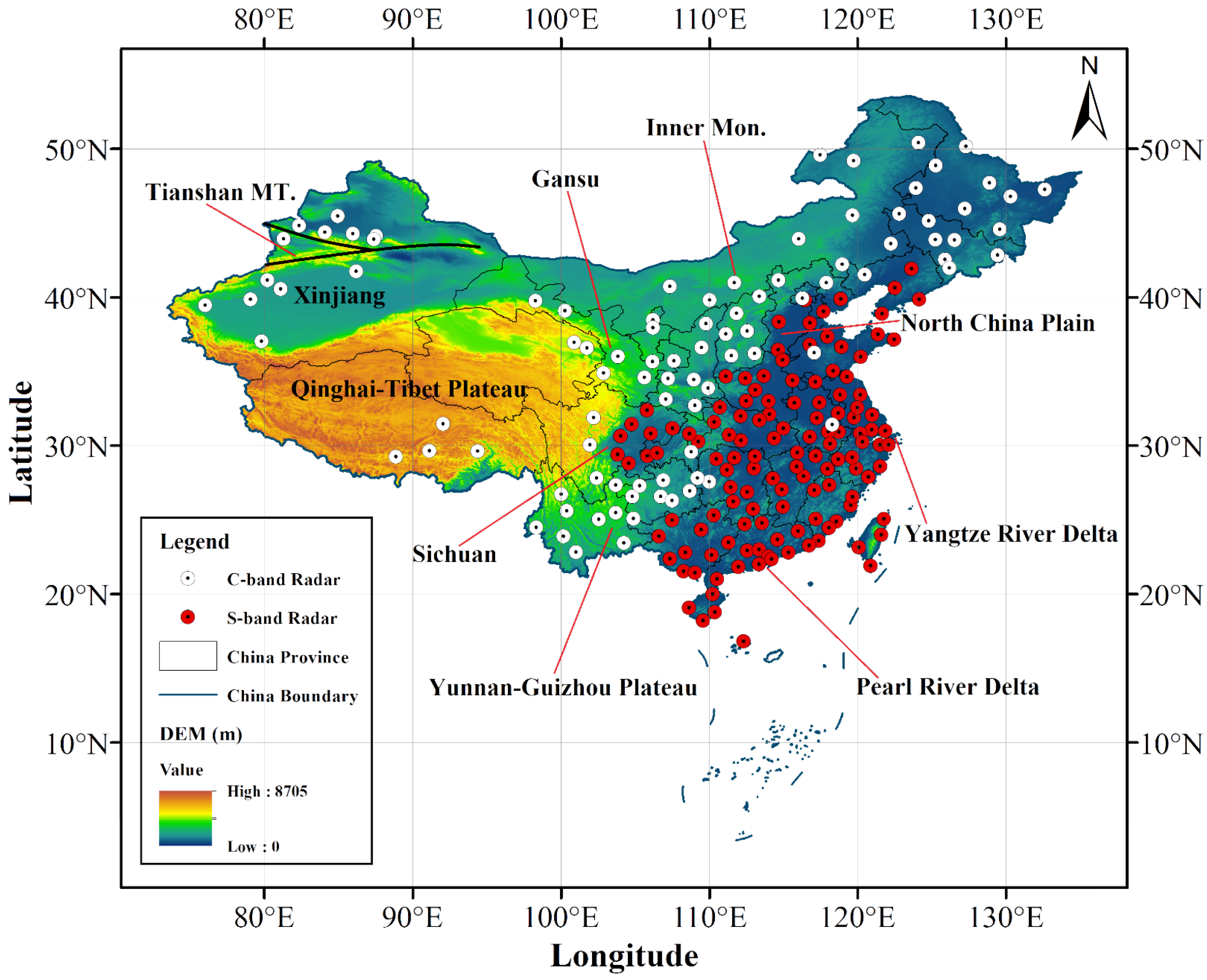
2.1. Radar Echo Reflectivity Data

The China Meteorological Administration (CMA) has deployed the China Next Generation Weather Radar (CINRAD) network. Currently, the CINRAD network is composed of 217 Doppler weather radars (94 C-band radars and 123 S-band radars) over mainland China (see Figure 1). These radars are distributed densely across China, except in complex terrain [44] and related radar echo data are used to locate precipitation events, calculate their motions and estimate their types (rain, snow, hail, etc.). Animations of radar products show the evolution of reflectivity and velocity patterns. We downloaded and collected five precipitation seasons (May to August) radar echo maps from 2017 to 2021 with a time interval of 6 min (the total length is 75,908 after data cleaning) and the coverage area is (73${}^{\circ }$E–135${}^{\circ }$E, 10${}^{\circ }$N–55${}^{\circ }$N). The basic steps for data cleaning include: extract the pixel values from the ‘RGB’ channel of the color echo map; match the pixel values with related radar echo reflectivities based on a given ‘reflectivity colorbar’; remove the annotations (e.g., city name, river name and border line) from each echo map and then use ‘Cressman’ interpolation method to fill in the related missing pixel values. We resample the reflectivity values on 1024 × 880 grids for each radar reflectivity map, while its actual spatial resolution is about 5 km. Finally, total samples with a size of 75,908 × 1024 × 880 are obtained.

2.2. Methods

In most DL architectures, convolution is the key operation for feature extraction of vision tasks, while ‘vanilla convolution’ is one of the most commonly used convolutions. Supposing x is the input feature of a vanilla convolution and K is the corresponding convolutional kernel, the output feature Y can be given by the following equation:

$$Y\left(p_0\right)={\mathsf{\Sigma }}_{p_n\in C}W\left(p_n\right)·x(p_0+p_n)$$

(1)

where $p_0$ is the current position in both input and output feature maps, $p_n$ is the position in receptive field C and W denotes the parameter of K. The vanilla convolution extracts features mainly by sparse connectivity and shared weights. However, it treats local cues as a weighted sum which may ease the detailed difference information locally [45]. Moreover, it lacks contextual information and accommodates uncertainty in the hierarchical inference process, so blurry/averaged prediction and cumulated error are obtained [46]. As for a precipitation forecasting task, the vanilla convolution may have difficulty in excavating the features of the precipitation field, such as moving speed, shape and intensity. To reduce the redundant and uncertain features in vanilla convolution, [47] proposed the split-based convolution (SPConv) which split the feature maps into the representative part and the redundant part, where the former applies $k\times k$ convolution to supply intrinsic features and the latter uses point-wise convolution to complement tiny hidden details. Inspired by this idea, we devise ‘time series residual convolution (TSRC)’ formulated as:

$$Y\left(p_0\right)={\mathsf{\Sigma }}_{p_n\in C}W\left(p_n\right)·(x^{[\tau +1]}(p_0+p_n)+\alpha ·{\overline{x}}^{\left[\tau \right]}(p_0+p_n))$$

(2)

$$Y\left(p_0\right)={\mathsf{\Sigma }}_{p_n\in C}W\left(p_n\right)·x^{[\tau +1]}(p_0+p_n)+\alpha ·\left({\overline{x}}^{\left[\tau \right]}(p_0+p_n)\right)·{\mathsf{\Sigma }}_{p_n\in C}W\left(p_n\right)$$

(3)

$${\overline{x}}^{\left[\tau \right]}(p_0+p_n)=\frac{1}{k}{\mathsf{\Sigma }}_{p_n\in C}^{k}x\left(p_n\right)$$

(4)

where $x^{[\tau +1]}$ denotes the input feature at time $\tau$ and $\tau +1$, ${\overline{x}}^{\left[\tau \right]}$ represents the input feature $x^{[\tau +1]}$ after ‘mean-expansion’ operation (see Figure 2b) at time $\tau$, respectively. $\alpha$ is the coefficient of $x^{[\tau +1]}$. Equation (3) is the expansion of Equation (2); it consists of the first term ‘vanilla convolution’ and the second term ‘residual module’. Equation (4) presents the solution procedure. Here, the corresponding local receptive field cube for 3D convolution is:

$$C=\left\{\right(-1,-1,-1),(-1,-1,0),\cdots ,(0,1,1),(1,1,1\left)\right\}$$

(5)

Our TSRC method is fortified with residual modules so that more information can be reserved. Because TSRC compensates the current local cues with previous local cues, so more contextual information and fewer uncertain feature would remain. Through such a convolution, the problem of information loss and cumulated errors can be alleviated to a certain extent. Therefore, we will use TSRC to tackle the decay of precipitation intensity and smoothing/blurry effect in real forecasting.

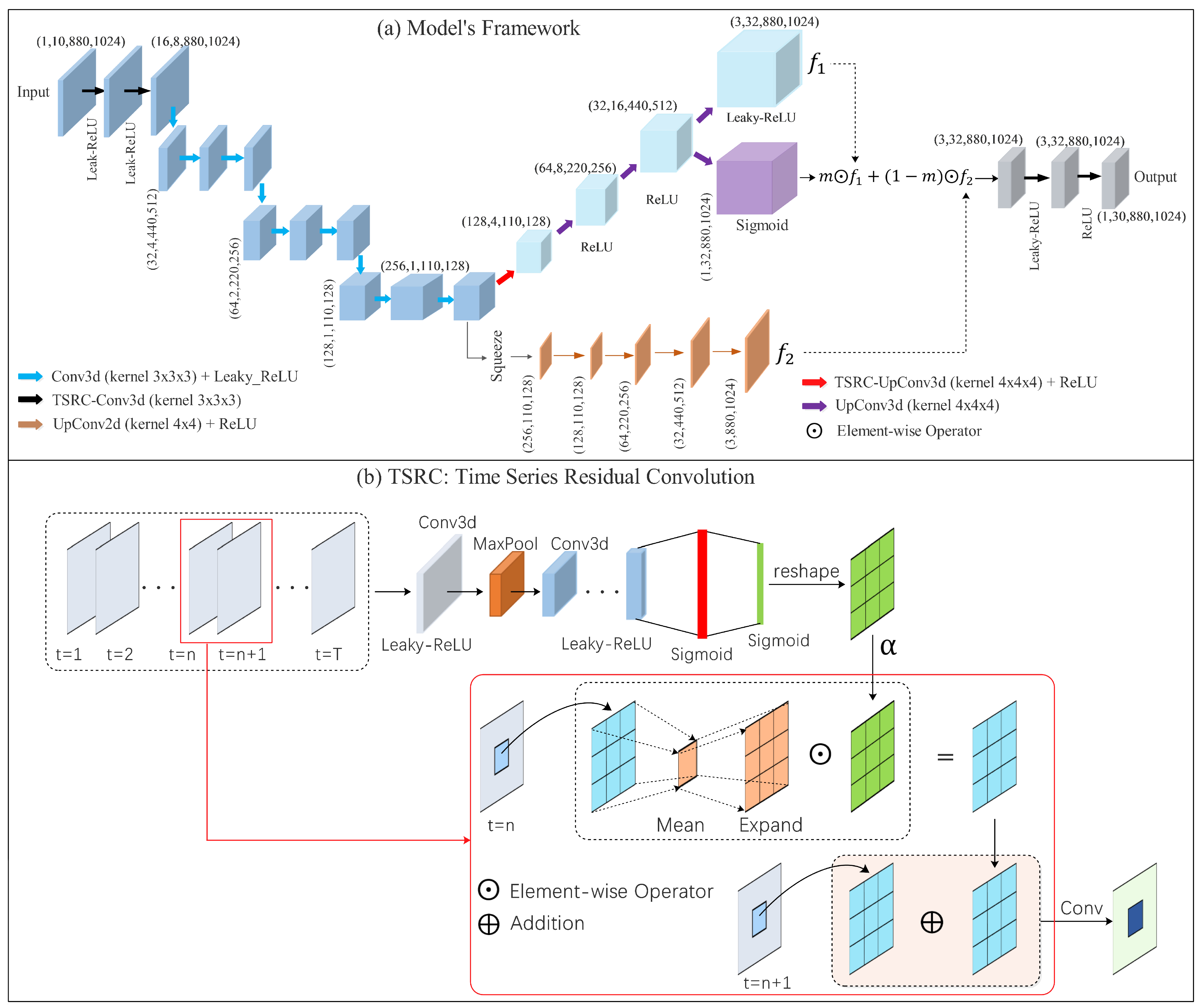
2.3. The Framework of the Model

Figure 2a shows the model’s framework in this study. Overall, the input size is $(10,H,W)$, while the output size is $(1,30,H,W)$, suggesting that the model uses 1 h previous radar reflectivity maps to conduct 3 h lead time precipitation forecasting. The main modules include the TSRC module (also see Figure 2b), 3D convolution layer, Leaky-ReLU layer, 2D up-convolution layer (2D up-sampling operator), 3D up-convolution layer (3D upsampling operator), ReLU layer, element-wise operator (Hadamard product), sigmoid activation layer, feature masking operator (the purple cube in Figure 2a). Basically, the framework consists of an encoder–decoder architecture which can be regarded as a procedure for information compression and feature extraction and several plug-and-play TSRC modules are also implanted into this architecture to help it retains more key features. From the prospective of spatial variation and time dependency of a precipitation system, these 3D TSRC modules struggle to capture movement characteristics of precipitation system such as the moving speed, falling area, intensity, propagation, generation and extinction. Suppose the output of the architecture is $f_1$, while one of the intermediate features is m, then an element-wise operation is performed (see $m⨀f_1$ in Figure 2a) to achieve the effect of feature masking (this can be explained as some kind of ‘attention mechanism’). The above operations are mainly used for feature extractions for radar echo maps at a 3D space-time scale. Apart from the above architecture, a 2D up-sampling operation is conducted, while this step is mainly used for feature extractions at a 2D space-time scale and it is supposed that its output is $f_2$. We combine the above features (see $m⨀f_1+(1-m)⨀f_2$ in Figure 2a) so that multi-scale information can be excavated as much as possible. In addition, the framework also implants some plug-and-play layers (e.g., ReLU, Leaky-ReLU, etc.) to ease vanishing gradients or exploding gradients.

It is noteworthy that the TSRC module uses a residual connection (see the ‘⨁’ operation in Figure 2b), so it can retain some information from previous time steps to a certain extent. Moreover, the TSRC module increases the depth of a hierarchical architecture with more parameters, so it can extract more potential features from the inputs. Therefore, more contextual information is retained in the TSRC module. In addition, our TSRC module implants ‘time series convolution’ (see ‘$Conv3d$’ operation in Figure 2b) so that it excavates the dependencies on both time-scale and space-scale; therefore, the less uncertain feature remains in this architecture. Theoretically, the ‘addiction’ operation in the TSRC module can postpone the declining rate of precipitation intensity to a certain extent, so the model is able to produce intensive echoes.

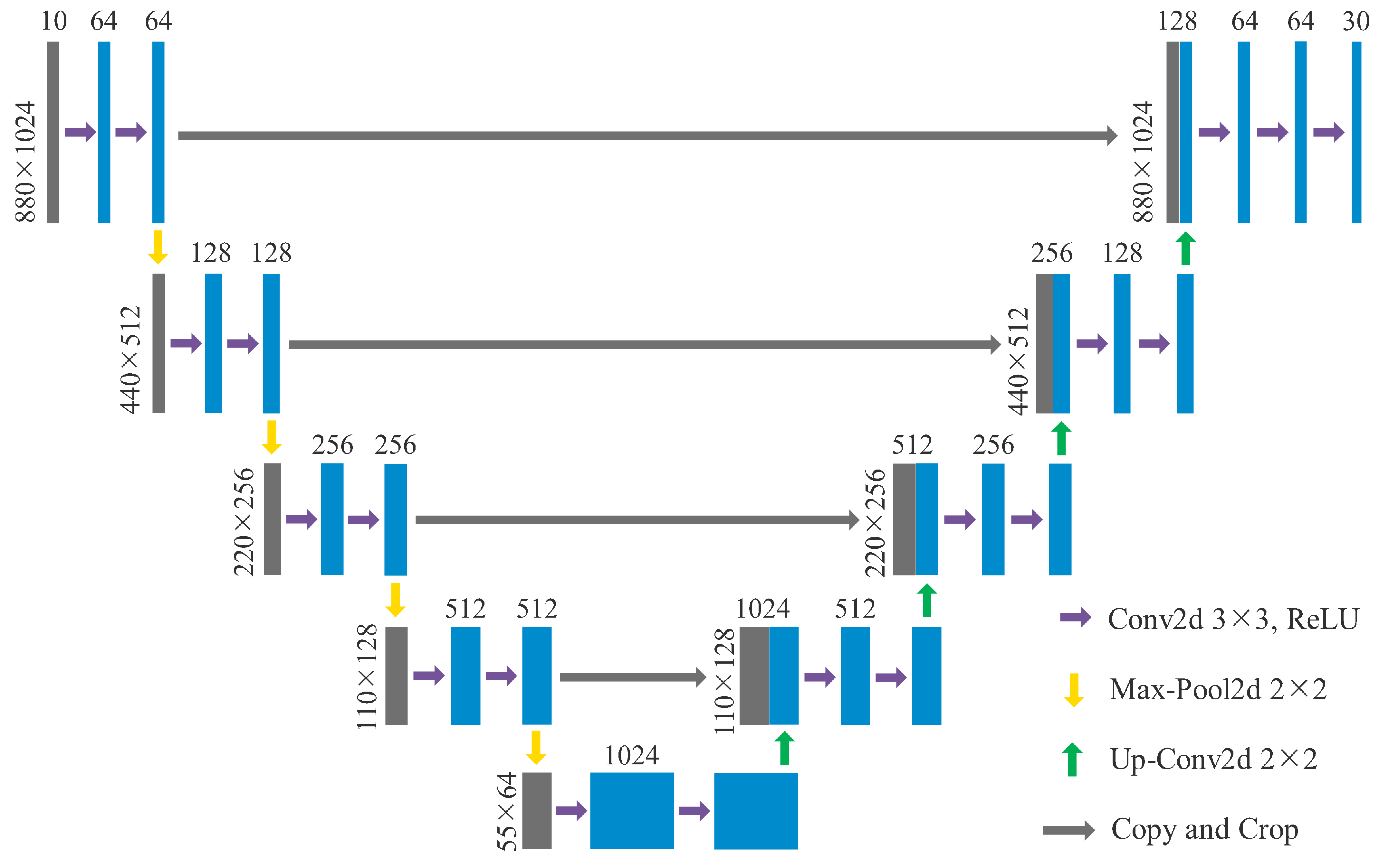
2.4. Reference Models

To have a better comparison with TSCR, we present the optical flow model (OF) and UNet model, which are two commonly used models in radar echo extrapolative forecasting.

The concept of “optical flow” was proposed by [48] and represents an instantaneous velocity of pixel motion of a moving object in an imaging plane. The core idea of OF is to calculate the optical flow field by introducing expedient restraint conditions. The calculation of OF usually holds two basic hypotheses: gray-scale invariance between neighbor pixels and micro-motion of radar echo. Let $(x,y)$ be the position of a pixel in a given echo map, and $I_t(x,y)$ be the corresponding gray value at time t. From t to $t+\Delta t$, the pixel moves to $(x+\Delta x,y+\Delta y)$, so its gray value is $I_{t+\Delta t}(x+\Delta x,y+\Delta y)$. Based on the gray-scale invariance hypothesis, the gray value before and after moving remains constant, so the following equation holds:

$$I_t(x,y)=I_{t+\Delta t}(x+\Delta x,y+\Delta y)$$

(6)

Additionally, based on the micro-motion hypothesis and Taylor expansion (ignoring the second-order infinitesimal), Equation (6) can be expanded as:

$$\frac{\partial I}{\partial x}\Delta x+\frac{\partial I}{\partial y}\Delta y+\frac{\partial I}{\partial t}\Delta t=0$$

(7)

Let $u=\frac{\Delta x}{\Delta t}$ and $v=\frac{\Delta y}{\Delta t}$ be two optical flow speeds at the x and y axes, respectively. Therefore, we have:

$$I_{x}u+I_{y}v+I_t=0$$

(8)

where $I_x=\frac{\partial I}{\partial x}$, $I_y=\frac{\partial I}{\partial x}$ and $I_t=\frac{\partial I}{\partial t}$ are the derivatives of the gray value I concerning $x,y$ and t, while u and v are two unknown variables. Therefore, to specify the value of OF, some constraint conditions are needed. Currently, there are mainly two methods to solve OF fields: global optical flow [49] and local optical flow [50]; details of algorithm derivations will not be given here.

The other reference model is UNet, which is a classic DL architecture and is widely used in image segmentation of the computer vision field [29]. The architecture mainly includes an encoder module and decoder module and related operations such as 2D convolution, down-sampling, up-sampling and skip connection. Because two feature extraction paths (encoder and decoder) are symmetrical to each other with a U-shape architecture, it is known as UNet. In this study, we develop UNet architecture (Figure 3) according to the specific inputs of the radar echo map. It can be seen from Figure 3 that both global information and local information of radar echo are well dispersed; also, this valid information will be retained by this U-shape architecture.

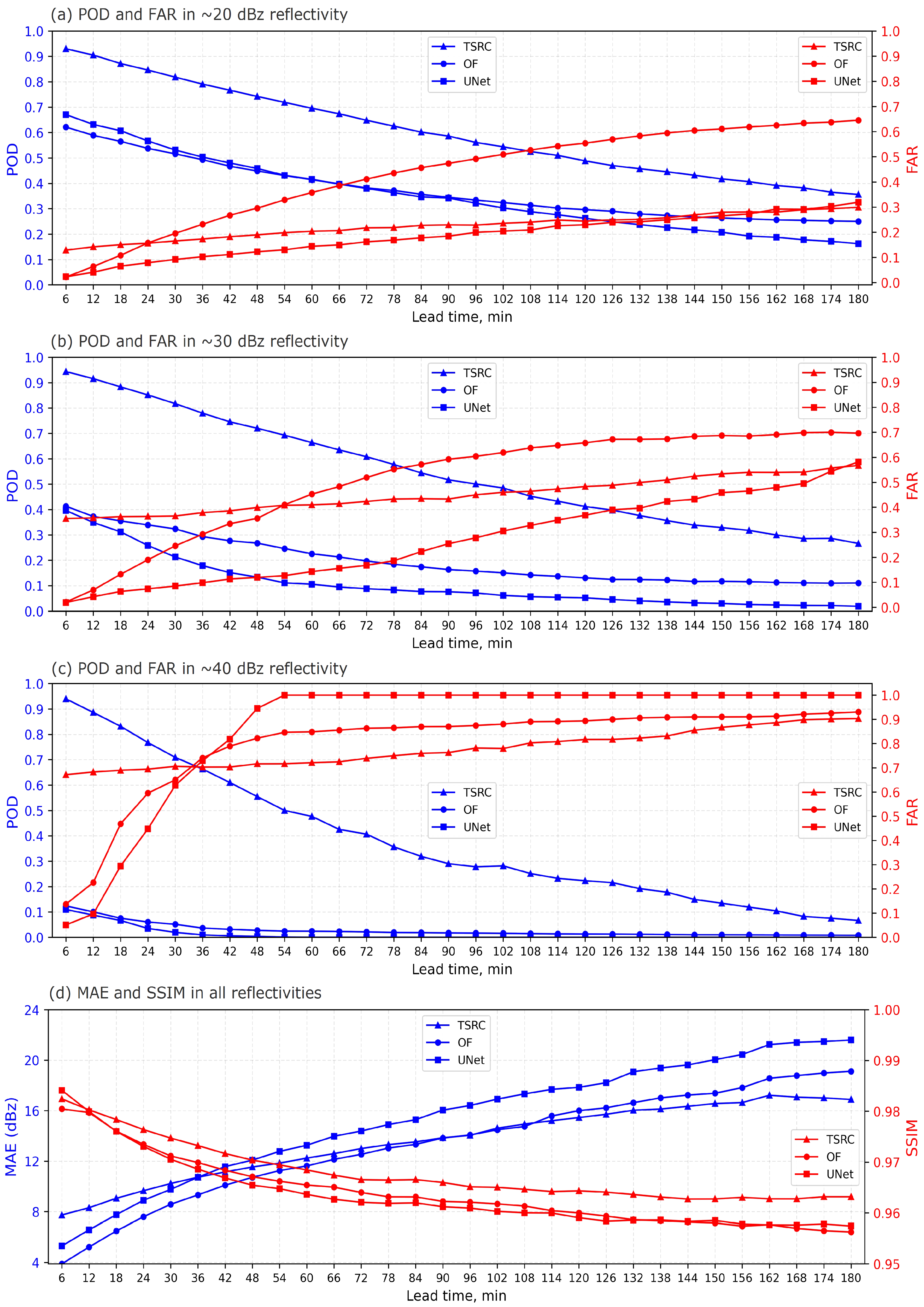
2.5. Evaluation Metrics

To evaluate the forecast performance of TSCR, OF and UNet, four evaluation metrics are used in this study, i.e., mean absolute error (MAE), probability of detection (POD), false alarm rate (FAR), radially averaged power spectral density and structural similarity index (SSIM).

$$MAE=\frac{1}{n}{\mathsf{\Sigma }}_{i=1}^n|Y_i^g-Y_i^f|$$

(9)

where $Y_i^g$ and $Y_i^f$ are ground truth and the forecast in the i-th pixel of the corresponding radar map and n is the number of pixels. This metric describes the forecast ability of each model under different precipitation intensities.

$$POD=\frac{n_s}{n_s+n_m}$$

(10)

$$FAR=\frac{n_f}{n_s+n_f}$$

(11)

where $n_s$, $n_m$ and $n_f$ represent successful forecast, missing forecast and null forecast, respectively. The above three values are determined by comparing the ground true value (GTV), the forecast value (FV) and the pre-defined threshold (PDT). In meteorology, the threshold of 20 dBz means those reflectivity values greater than or equal to 20 dBz; hereafter, it will be abbreviated as ‘∼20 dBz’. Similarly, the term ‘∼30 dBz’ and ‘∼40 dBz’ can be used. In this study, the thresholds are set to ∼20, ∼30 and ∼40 dBz. For example, if GTV ≥ PDT and FV ≥ PDT, then mark one successful forecast; if GTV ≥ PDT and FV < PDT then mark one missing forecast; if GTV < PDT and FV ≥ PDT, then mark one null forecast. Both POD and FAR intuitively present the forecast performance at different precipitation intervals.

The mathematical derivation of power spectral density is referred to in Sinclair’s work [51]; the details are left out here. We calculate radially averaged power spectral density [52] to examine the problem of over-smoothing or flattening forecasts in different models.

In addition, in order to investigate the deterioration problem with increasing lead times and the decay of precipitation intensity, we calculate the mean of echo intensity formulated as:

$$SSIM=\frac{(2{\mathsf{\mu }}_g{\mathsf{\mu }}_f+c_1)(2{\mathsf{\sigma }}_{gf}+c_2)}{({\mathsf{\mu }}_g^2+{\mathsf{\mu }}_f^2+c_1)({\mathsf{\sigma }}_g^2+{\mathsf{\sigma }}_f^2+c_2)}$$

(12)

where ${\mathsf{\mu }}_g$ and ${\mathsf{\mu }}_f$ are the mean value of the ground truth radar map and the forecast map, ${\mathsf{\sigma }}_g$ and ${\mathsf{\sigma }}_f$ are the corresponding standard deviation, ${\mathsf{\sigma }}_{gf}$ is the covariance. $c_1$ and $c_2$ are two constants. The mathematical derivation of SSIM refers to Wang’s work [53]. This metric is used for measuring the similarity between the ground true radar map and the forecast map.

3. Results

3.1. Overall Forecast Results on Testing Data

Here we present the forecast results of TSRC, OF and UNet which uses the radar reflectivity data over 2021 as the testing data. Figure 4 shows the four evaluation metrics POD, FAR, MAE and SSIM with the three radar reflectivity intervals ∼20, ∼30 and ∼40 dBz. Obviously, PODs in TSRC are higher than in OF and UNet for all three reflectivity intervals. At least PODs with the value of 0.5 in TSRC can be maintained 2 h, 96 min and 1 h in three reflectivity intervals, respectively, suggesting that our model yields almost half of the successful forecasts in the lead time of 2 h, 96 min and 1 h. Another finding is that for TSRC, there are linear decrease tendencies in PODs with increased forecast times. In contrast, for both OF and UNet, the whole PODs are less than 0.4 in ∼30 dBz reflectivity and are almost near 0 for all forecast times in ∼40 dBz reflectivity, suggesting that it is quite difficult to forecast strong precipitations with the two models, especially for long-range forecasting.

In terms of FAR, for all three reflectivity intervals, it is easy to find that FARs for TSRC climb slowly from 12 min to 3 h forecast times. In contrast, the increasing trends of FARs for both OF and UNet are relatively steep. In ∼20 and ∼30 dBz reflectivity intervals, although UNet acquires relatively low FARs, the PODs are also low, while the reverse occurs in TSRC. Note that in ∼40 reflectivity intervals, OF and UNet both produce lower FARs than in TSRC before 36 min lead times, but they rapidly climb to 0.8 at 1 h lead times, while all three models obtain relatively high FARs after 1 h lead time. Overall, our model ranks the best forecast after 1 h lead times.

We calculate the MAE and SSIM between ground truth and forecasts. It can be found that MAEs in the three models increase with lead times. Specifically, OF has the lowest MAEs before the 84 min lead time, while TSRC has the lowest MAEs after 2 h lead time, UNet acquires relatively greater MAEs than the other two models beginning at 36 min lead time, these indicating that OF is more appropriate for predicting precipitation intensity for the first hour while TSRC is for the last 2 h. As for SSIM, TSRC performs the best with SSIM values greater than 0.96, followed by OF and UNet, suggesting that TSRC reproduces the shapes of the precipitation field with relatively high similarity. According to the analysis of MAE and SSIM, it can be found that OF is more prone to predicting short-range precipitation, while TSRC shows its unexampled advantage in producing long-range precipitation fields (both intensities and shapes) and UNet has a poor capacity to predict precipitation fields.

To sum up the above results, our model TSRC performs the best in long-range forecasts, OF shows certain superiority in short-range forecasts and UNet has poor ability in both long-range and short-range forecasts. Some possible reasons include the following: OF produces precipitation fields based on assumptions of Lagrangian persistence and smooth motion fields; however, it cannot trace the fast changes of precipitation fields in short-range times [8,54], while it also brings about cumulated errors due the discrepancy between training and test objectives from short-range to long-range forecasts. UNet is essentially a 2D CNN-based DL architecture; it implements convolution operations only on a spatial dimension, which easily causes information loss and is unfavorable for extracting spatial-temporal features of radar reflectivity. Meanwhile, the encoder–decoder module inevitably introduces information losses; therefore, it is difficult to capture the changes in precipitation fields. TSRC compensates the current spatial-temporal features of radar reflectivity with previous ones so that the information loss problem and cumulated errors can be alleviated.

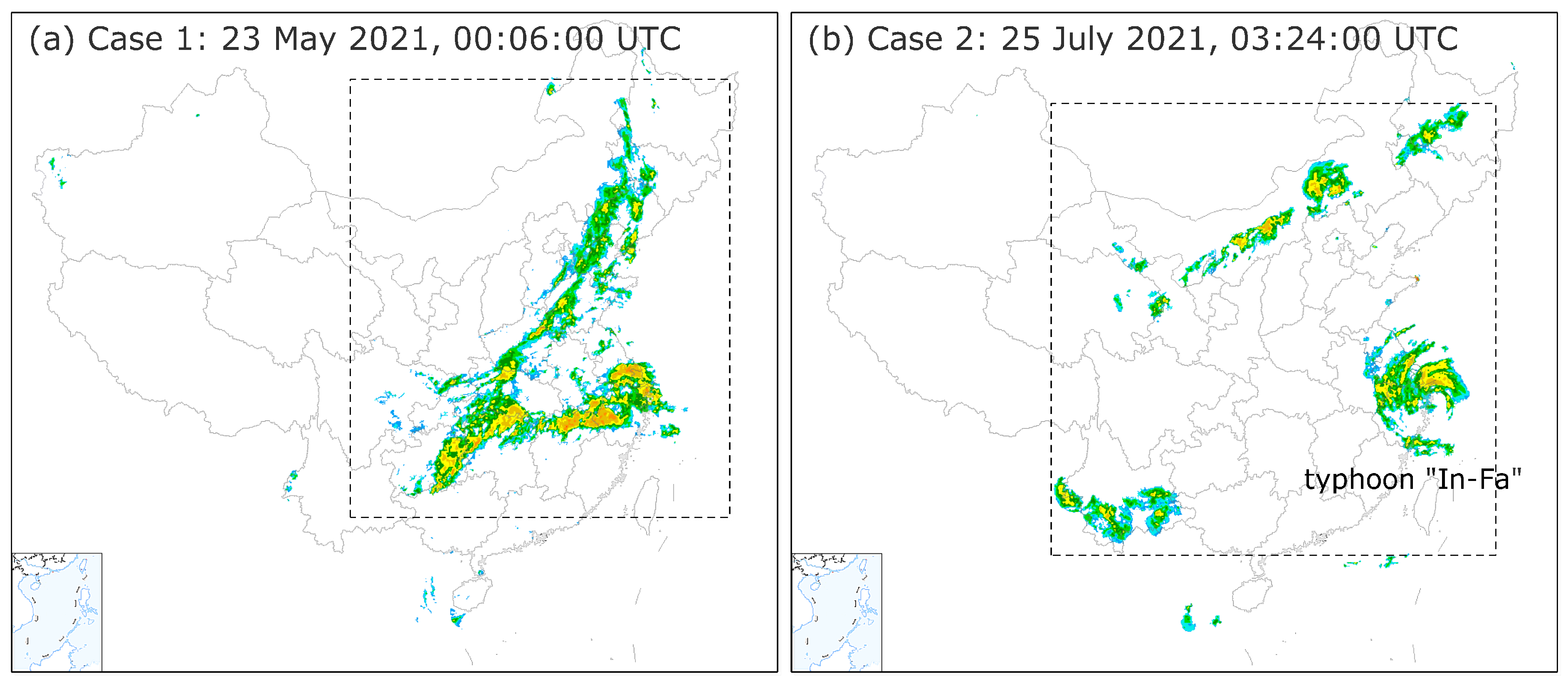
3.2. Results of Case Study

Here we present two case studies (Figure 5) to further understand the forecast performances of three models.

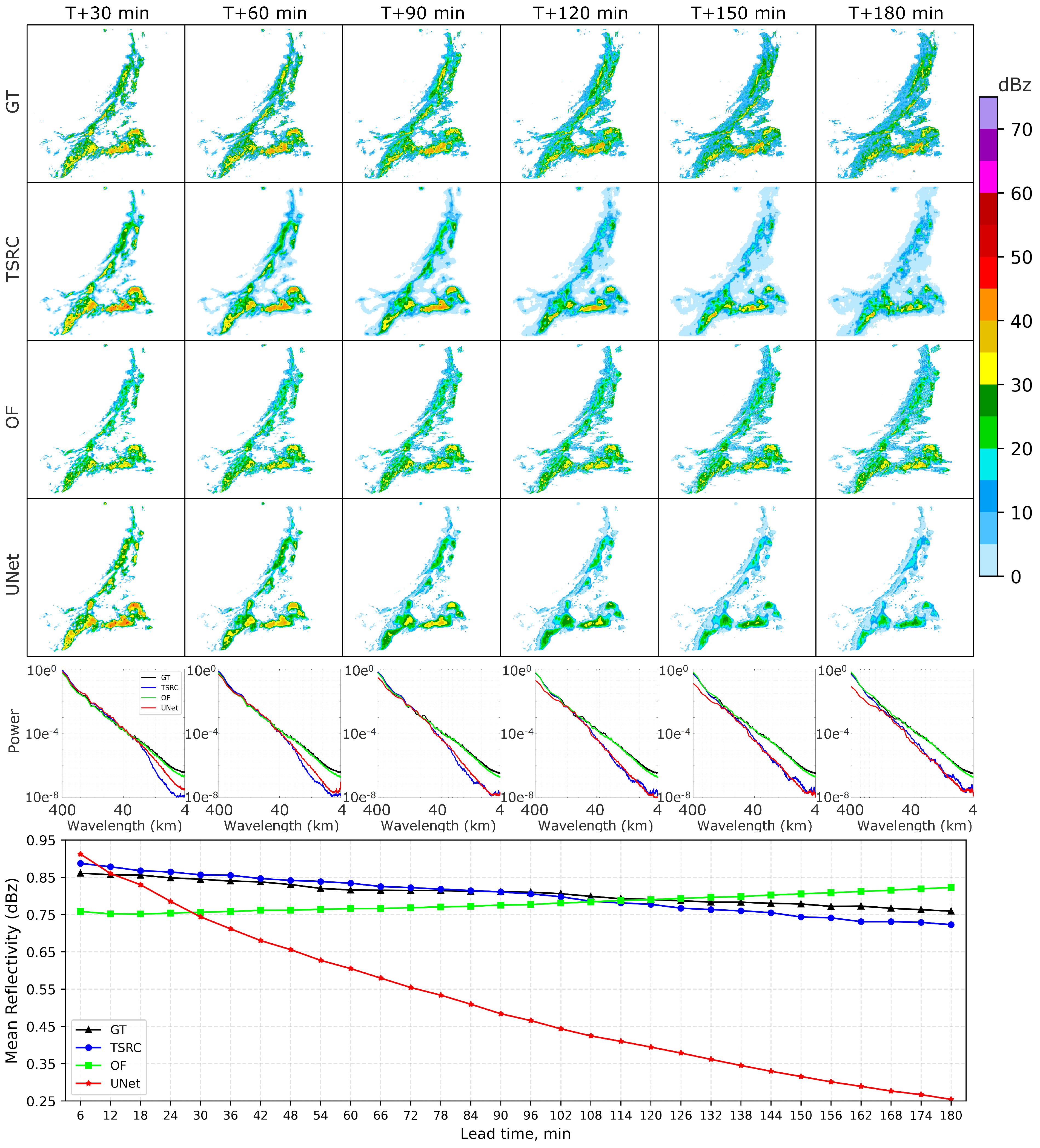
3.2.1. Case 1

The first precipitation case happened on 23 May 2021, 00:06:00 UTC (Figure 5a); it was a large-scale rainfall covering most of China. Figure 6-top presents the forecast results of TSRC, OF and UNet. As can be seen from ground truth (GT), the rainfall area unobtrusively enlarged with increased lead times, but the high-intensity area (>40 dBz) gradually became more centralized. In terms of the rainfall area, TSRC shows the best forecast skill. Though OF depicts rough rainfall shapes, they are more like depictions of precipitation fields from shorter lead time to longer lead time, which can also be found from a string of trajectories of rainfall fields. In other words, OF only shifts the rainfall fields at a horizontal scale and ignores the local changes in the rainfall field; that is the reason why the differences in rainfall area from the first lead time to the last lead time are very slight; this raises the question of whether OF can forecast rapid changes of rainfall field, especially long-term forecasts. UNet performs poorly in rainfall area forecasting when a degradation problem of precipitation field is striking and the missing forecasts increase with forecast lead times. In addition, through a delicate investigation, the problem of generation and extinction is conspicuous in both OF and UNet, while this problem has been partly improved by TSRC.

The plots of radially averaged power spectral density (Figure 6-middle) provide a more intuitive method to evaluate the smoothing effect on three forecast models, while the lower the power, the more serious the smoothing effect will be. Obviously, OF has the weakest smoothing effect and it outperforms the other two models for all forecast times. According to the discussion above, OF performs well in shorter lead time and the rainfall fields of longer lead time are almost copied from previous forecast frames; that is the reason why OF introduces relatively meticulous rainfall fields. In contrast to OF, the two DL-based models TSRC and UNet inevitably bring in the smoothing effect. For the first 90 min forecast times, TSRC achieves the lowest power at wavelength < 40 km, while for the last 90 min forecast times TSRC’s power is slightly improved compared to UNet. It is a generally existing problem that most DL-based models unavoidably report smoothing forecasts due to the use of convolutional operation; consequently, their forecast rainfall fields are usually smoother than that from OF ([24,28]).

We calculate the mean reflectivity (Figure 6-bottom) to examine the performance of reflectivity intensity forecasting at different lead times. Evidently, UNet performs poorly and the cumulated error increases with forecast lead time; it cannot capture radar echo shapes and substantially underestimates radar echo intensities, especially at longer lead times, this is confirmed by the low POD and high FAR in high-intensity echo forecasting (see POD and FAR in Figure 4). Comparatively, TSRC ranks the best for all forecast lead times since the errors are smallest and it follows the same trend of echo intensity as in GT; therefore, it can efficiently extrapolate the radar echo evolution at longer lead times. Conversely, although OF also obtains small forecast errors; however, it follows the opposite trend of echo intensity and underestimates the echoes in the first 2 h lead times and overestimates the echoes in the last hour. In other words, OF simply preserves echo intensities over all forecast times and is unable to capture the temporal correlations and spatial information of the rainfall field.

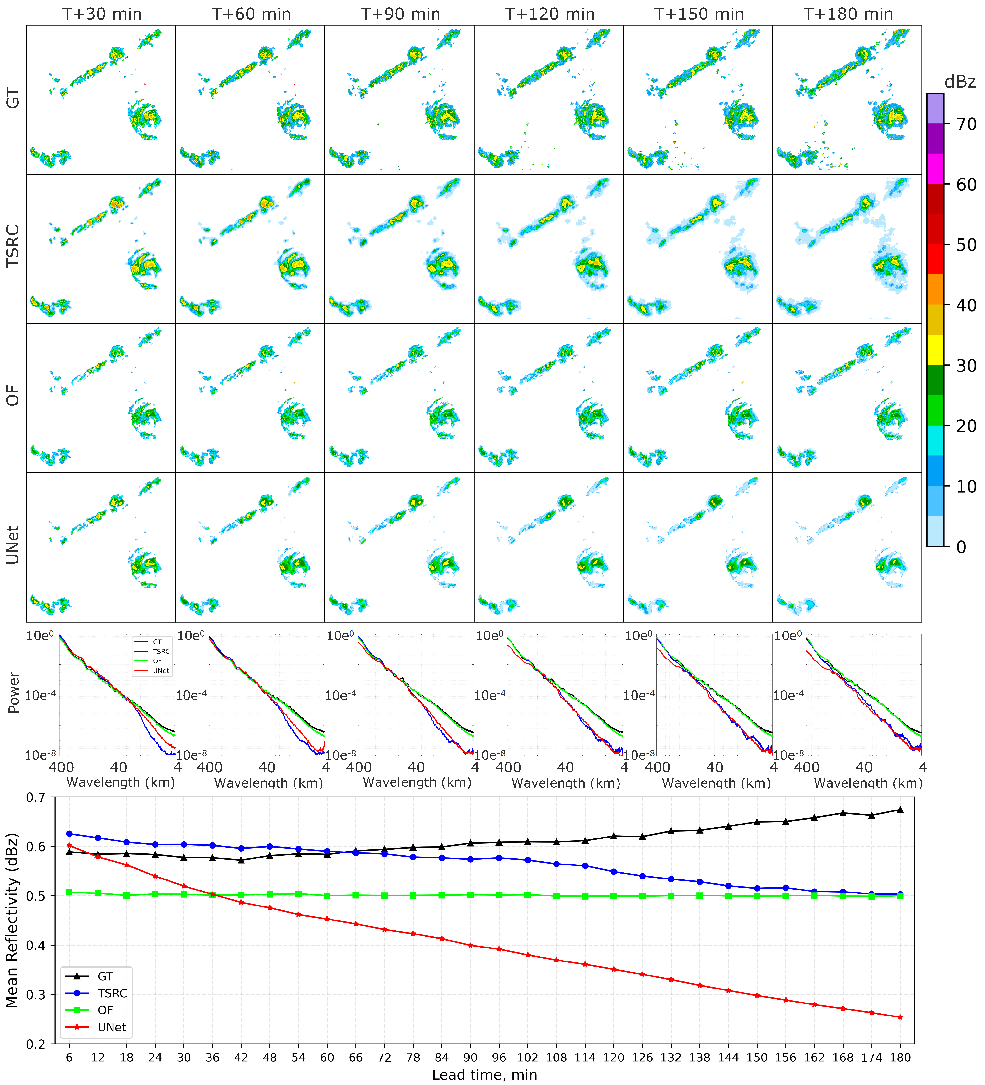
3.2.2. Case 2

This case occurred on 25 July 2021, 03:24:00 UTC (Figure 5b) and includes a rainfall process influenced by severe typhoon In-Fa and two isolated convective precipitations influenced by a high-level trough and warm-moist air in the low level. Figure 7 shows the forecast results of the three models. In GT, we can observe that the falling areas of convective precipitation slowly expand, while the high-intensity echo areas are sporadic-like distributions and the counterclockwise rotation is clear from the spiral rainband of In-Fa. TSRC roughly reproduces the shapes of convective precipitation and the spiral rainband. For OF, unsurprisingly, it exhibits almost the same echo maps in all forecast lead times and hence has limited ability to provide the local features of convective precipitation and spiral rainband. For UNet, the shapes of both spiral rainband and convective precipitation degenerate seriously; hence, most missing forecasts can be found.

The three models introduce different levels of smoothing effect, especially TSRC and UNet. Specifically, in shorter forecast lead times (first 1 h), TSRC shows the lowest power at a wavelength of <40 km, while in longer lead times TSRC and UNet show similar smoothing effects. It is indisputable that OF yields the lowest level of smoothing effect because the rainfall fields rarely change over all forecast lead times. In terms of the mean echo intensity, UNet shows the worst performance and OF keeps a relatively stable performance at shorter lead times but sorely underestimates the echo intensity at longer lead times. TSRC obtains the most proper echo intensity at the first hour while its performance begins to decline at a lead time of 2 h (at least echo intensity > 35 dBz at a lead time of 3 h can be found only in TSRC). To sum up the above results, TSRC demonstrates a certain advantage in handling the forecast of typhoon rainfall compared to the simply extrapolated method OF and the DL-based method UNet. However, due to the complex law of cyclone propagation, both rainfall shape forecasting and echo intensity forecasting still need to be improved in all models.

4. Discussions

Here we summarize the three models’ advantages and disadvantages. From a quantitative point of view, the calculation of OF is based on the changes of echo and the correlation of two adjacent echo maps; it seeks the relationship of different maps and lastly determines the information of echo motion and the change of echo intensity in a motion vector field. Therefore, OF can accurately track and predict the moving object in an echo map. The advantage of OF is that it obtains considerable success in forecasting precipitation systems of slow change in the short term. Meanwhile, OF submits to the hypotheses of gray-scale invariance in radar echoes, but there are rapid generations and extinctions in strong convection systems which will make OF produce relatively large forecast errors due to the non-conservation radar echo reflectivities. In a word, OF shows poor forecast skills in strong convection. Moreover, strong convection is a highly complex and nonlinear system and is usually accompanied by rotary motion which will result in great discrepancies between extrapolative echoes and ground truth due to the linear extrapolation of the optical flow field. Even with further improved methods such as the semi-Lagrangian method relying on the advection equation, it is still difficult to unravel the vorticose structures of precipitation systems. Therefore, OF performs poorly in operational forecasting tasks such as precipitation systems with rapid change, typhoon precipitation systems and strong convection systems.

UNet is essentially an encoder–decoder DL architecture; its advantages are as follows: there are clear feature representations in different network frames, whereas deep network frames with greater receptive fields focus on those global (abstract or essential) features of precipitation systems; in contrast, shallow network frames pay more attention to local and textured features of the precipitation system; the upsampling operation in UNet may lead to information losses on the image edge, while those losses can be supplemented by conducting feature concatenation layers in UNet. The disadvantage is it has a contradiction between receptive fields and information losses: greater receptive fields need more pooling layers for feature dimension reduction, which lead to more information losses; in contrast, smaller receptive fields are incompetent in terms of capturing global or large-scale features, thus also leading to information losses. In addition, UNet conducts convolution only on a spatial scale; nonetheless, radar echoes have variability at various temporal and spatial scales, so it is not insufficient for UNet to capture spatial-temporal features of radar echo. Consequently, UNet performs poorly in forecasting the shape of the precipitation system and the echo intensity; also its forecast skill rapidly deteriorates with lead time.

The main objectives of TSRC in this study are to alleviate two issues: the smoothing effect in forecast precipitation and the degenerate effect of forecasting precipitation intensity. The forecasting results, from a quantitative point of view at least, suggest that our model achieves relatively superior forecast performances in several evaluation metrics: POD, FAR, MAE and SSIM. Two rainfall cases show that with TSRC it is unavoidable to report a smoothing effect (it underperforms the OF but outperforms UNet); of course, this is not specific to our model and most DL-based models must also contend with the same issue. The most prominent result is that TSRC can yield high-intensity radar echoes even in typhoon precipitation systems while both OF and UNet cannot, illuminating that the degenerate effect of forecasting precipitation intensity can be alleviated in our model. Specifically, two issues (information loss and cumulated error) will be inevitable in most DL-based models as long as convolutions are used, resulting in many practical forecasting problems such as the smoothing effect, the degenerate effect of echo intensity, the generation and extinction of rainfall field, the propagation of precipitation system, etc. Basically, TSRC also contains an encoder–decoder DL architecture which is as essential to information compression and feature extraction for radar echo maps. In addition, TSRC skillfully utilizes the ‘residual module’ term so that a past radar echo feature at previous time steps can be retained to a certain degree. There are also two design tricks in TSRC, such as intermediate feature masking, feature fusion, etc. Theoretically, all the above operations in TSRC are conducive to alleviating the smoothing effect and reducing cumulated errors accordingly and they are also confirmed by the forecast results in this study at least. At any rate, TSRC is a pure data-driven radar echo extrapolation model which fails to take physical constraints and atmospheric dynamics into consideration. However, merely TSRC achieving several inspiring evaluation metrics does not represent the limit of TSRC performance reached. In the future, from an early warning perspective, great efforts are still necessary to improve TSRC’s forecasting skills and further make practical applications.

5. Conclusions

We propose a DL-based architecture TSRC for the radar echo short-term (3 h) forecasting over China and this model is compared to two commonly used extrapolation methods: OF and UNet. We test the three models using radar echo data throughout 2021 and analyse two specific precipitation events. Results show that TSRC achieves the most impressive forecasting skills with relatively high POD and low FAR compared with OF and UNet, especially for high-intensity radar echo. The forecast results from two rainfall cases suggest that TSRC yields acceptable outlines of rainfall fields and produces relatively high-intensity echoes at longer forecast lead times; by contrast, OF and UNet cannot do this. The smoothing effect is an eternal topic in DL-based models, both TSRC and UNet inevitably introduce different levels of the smoothing effect. Although the smoothing effect in OF is minimal, nonetheless it is not appropriate for long-term forecasting. From a statistical perspective, all three models are essentially radar echo extrapolations based on the characteristic of the previous echo advection field.

The short-term precipitation nowcasting models in this study only consider multi-time radar echoes as the training inputs; however, any meteorological data (e.g., wind field, air temperature, humidity, etc.) and underlying surface information could also be considered in the future. These data include but are not limited to radar echoes, satellite images, reanalysis data, real-time observations, output from NWP, etc. The combination of multi-source data may provide a measure of physical constraints or data assimilation for a pure data-driven precipitation nowcasting model. Currently, the smoothing effect in forecast precipitation and the degenerate effect of forecasting precipitation intensity are two thorny problems in most DL-based models. Apart from the combination of multi-source data, some reasonable adjustments on convolution or feature extraction modules seem desirable, such as ‘Deep Forest’ [55], axial self-attention in MetNet [25], 3D Earth-Specific Transformer in Pangu-Weather [26], skip connection in RainNet [24] and Fourier neural operators in FourCastNet [56]. Moreover, TSRC performs precipitation nowcasting tasks over China with a lead time of 3 h; future works should focus on how to extend the forecast time and expand the forecast area and how to balance the computational/time resource and the forecast accuracy.

References

- Ehsani, M.R.; Zarei, A.; Gupta, H.V.; Barnard, K.; Behrangi, A. Nowcasting-Nets: Deep Neural Network Structures for Precipitation Nowcasting Using IMERG. arXiv 2021, arXiv:2108.06868. [Google Scholar]
- Sun, J.; Xue, M.; Wilson, J.W.; Zawadzki, I.; Ballard, S.P.; Onvlee-Hooimeyer, J.; Joe, P.; Barker, D.M.; Li, P.W.; Golding, B.; et al. Use of NWP for nowcasting convective precipitation: Recent progress and challenges. Bull. Am. Meteorol. Soc. 2014, 95, 409–426. [Google Scholar] [CrossRef]
- Bauer, P.; Thorpe, A.; Brunet, G. The quiet revolution of numerical weather prediction. Nature 2015, 525, 47–55. [Google Scholar] [CrossRef]
- Yano, J.I.; Ziemiański, M.Z.; Cullen, M.; Termonia, P.; Onvlee, J.; Bengtsson, L.; Carrassi, A.; Davy, R.; Deluca, A.; Gray, S.L.; et al. Scientific challenges of convective-scale numerical weather prediction. Bull. Am. Meteorol. Soc. 2018, 99, 699–710. [Google Scholar] [CrossRef]
- Germann, U.; Zawadzki, I. Scale-dependence of the predictability of precipitation from continental radar images. Part I: Description of the methodology. Mon. Weather. Rev. 2002, 130, 2859–2873. [Google Scholar] [CrossRef]
- Germann, U.; Galli, G.; Boscacci, M.; Bolliger, M. Radar precipitation measurement in a mountainous region. Q. J. R. Meteorol. Soc. J. Atmos. Sci. Appl. Meteorol. Phys. Oceanogr. 2006, 132, 1669–1692. [Google Scholar] [CrossRef]
- Sokol, Z.; Mejsnar, J.; Pop, L.; Bližňák, V. Probabilistic precipitation nowcasting based on an extrapolation of radar reflectivity and an ensemble approach. Atmos. Res. 2017, 194, 245–257. [Google Scholar] [CrossRef]
- Prudden, R.; Adams, S.; Kangin, D.; Robinson, N.; Ravuri, S.; Mohamed, S.; Arribas, A. A review of radar-based nowcasting of precipitation and applicable machine learning techniques. arXiv 2020, arXiv:2005.04988. [Google Scholar]
- Yan, Q.; Ji, F.; Miao, K.; Wu, Q.; Xia, Y.; Li, T. Convolutional residual-attention: A deep learning approach for precipitation nowcasting. Adv. Meteorol. 2020, 2020, 6484812. [Google Scholar] [CrossRef]
- Weisman, M.L.; Davis, C.; Wang, W.; Manning, K.W.; Klemp, J.B. Experiences with 0–36-h explicit convective forecasts with the WRF-ARW model. Weather. Forecast. 2008, 23, 407–437. [Google Scholar] [CrossRef]
- Czibula, G.; Mihai, A.; Albu, A.I.; Czibula, I.G.; Burcea, S.; Mezghani, A. AutoNowP: An Approach Using Deep Autoencoders for Precipitation Nowcasting Based on Weather Radar Reflectivity Prediction. Mathematics 2021, 9, 1653. [Google Scholar] [CrossRef]
- Singh, M.; Kumar, B.; Rao, S.; Gill, S.S.; Chattopadhyay, R.; Nanjundiah, R.S.; Niyogi, D. Deep learning for improved global precipitation in numerical weather prediction systems. arXiv 2021, arXiv:2106.12045. [Google Scholar]
- Patel, M.; Patel, A.; Ghosh, D. Precipitation nowcasting: Leveraging bidirectional lstm and 1d cnn. arXiv 2018, arXiv:1810.10485. [Google Scholar]
- Chen, L.; Cao, Y.; Ma, L.; Zhang, J. A Deep Learning-Based Methodology for Precipitation Nowcasting With Radar. Earth Space Sci. 2020, 7, e2019EA000812. [Google Scholar] [CrossRef]
- Zheng, K.; Liu, Y.; Zhang, J.; Luo, C.; Tang, S.; Ruan, H.; Tan, Q.; Yi, Y.; Ran, X. GAN–argcPredNet v1.0: A generative adversarial model for radar echo extrapolation based on convolutional recurrent units. Geosci. Model Dev. 2022, 15, 1467–1475. [Google Scholar] [CrossRef]
- LeCun, Y.; Bengio, Y.; Hinton, G. Deep learning. Nature 2015, 521, 436–444. [Google Scholar] [CrossRef]
- Ayzel, G.; Heistermann, M.; Sorokin, A.; Nikitin, O.; Lukyanova, O. All convolutional neural networks for radar-based precipitation nowcasting. Procedia Comput. Sci. 2019, 150, 186–192. [Google Scholar] [CrossRef]
- Kim, D.K.; Suezawa, T.; Mega, T.; Kikuchi, H.; Yoshikawa, E.; Baron, P.; Ushio, T. Improving precipitation nowcasting using a three-dimensional convolutional neural network model from Multi Parameter Phased Array Weather Radar observations. Atmos. Res. 2021, 262, 105774. [Google Scholar] [CrossRef]
- Xue, M.; Hang, R.; Liu, Q.; Yuan, X.T.; Lu, X. CNN-based near-real-time precipitation estimation from Fengyun-2 satellite over Xinjiang, China. Atmos. Res. 2021, 250, 105337. [Google Scholar] [CrossRef]
- Yao, G.; Liu, Z.; Guo, X.; Wei, C.; Li, X.; Chen, Z. Prediction of Weather Radar Images via a Deep LSTM for Nowcasting. In Proceedings of the 2020 International Joint Conference on Neural Networks (IJCNN), Glasgow, UK, 19–24 July 2020; pp. 1–8. [Google Scholar]
- Luo, C.; Li, X.; Wen, Y.; Ye, Y.; Zhang, X. A Novel LSTM Model with Interaction Dual Attention for Radar Echo Extrapolation. Remote Sens. 2021, 13, 164. [Google Scholar] [CrossRef]
- Bai, S.; Kolter, J.Z.; Koltun, V. An empirical evaluation of generic convolutional and recurrent networks for sequence modeling. arXiv 2018, arXiv:1803.01271. [Google Scholar]
- Sadeghi, M.; Nguyen, P.; Hsu, K.; Sorooshian, S. Improving near real-time precipitation estimation using a U-Net convolutional neural network and geographical information. Environ. Model. Softw. 2020, 134, 104856. [Google Scholar] [CrossRef]
- Ayzel, G.; Scheffer, T.; Heistermann, M. RainNet v1. 0: A convolutional neural network for radar-based precipitation nowcasting. Geosci. Model Dev. 2020, 13, 2631–2644. [Google Scholar] [CrossRef]
- Sønderby, C.K.; Espeholt, L.; Heek, J.; Dehghani, M.; Oliver, A.; Salimans, T.; Agrawal, S.; Hickey, J.; Kalchbrenner, N. Metnet: A neural weather model for precipitation forecasting. arXiv 2020, arXiv:2003.12140. [Google Scholar]
- Bi, K.; Xie, L.; Zhang, H.; Chen, X.; Gu, X.; Tian, Q. Pangu-Weather: A 3D High-Resolution Model for Fast and Accurate Global Weather Forecast. arXiv 2022, arXiv:2211.02556. [Google Scholar]
- Ravuri, S.; Lenc, K.; Willson, M.; Kangin, D.; Lam, R.; Mirowski, P.; Fitzsimons, M.; Athanassiadou, M.; Kashem, S.; Madge, S.; et al. Skilful precipitation nowcasting using deep generative models of radar. Nature 2021, 597, 672–677. [Google Scholar] [CrossRef] [PubMed]
- Li, D.; Liu, Y.; Chen, C. MSDM v1. 0: A machine learning model for precipitation nowcasting over eastern China using multisource data. Geosci. Model Dev. 2021, 14, 4019–4034. [Google Scholar] [CrossRef]
- Ronneberger, O.; Fischer, P.; Brox, T. U-net: Convolutional networks for biomedical image segmentation. In Proceedings of the International Conference on Medical Image Computing and Computer-Assisted Intervention, Munich, Germany, 5–9 October 2015; Springer: Cham, Switzerland, 2015; pp. 234–241. [Google Scholar]
- Agrawal, S.; Barrington, L.; Bromberg, C.; Burge, J.; Gazen, C.; Hickey, J. Machine learning for precipitation nowcasting from radar images. arXiv 2019, arXiv:1912.12132. [Google Scholar]
- Lebedev, V.; Ivashkin, V.; Rudenko, I.; Ganshin, A.; Molchanov, A.; Ovcharenko, S.; Grokhovetskiy, R.; Bushmarinov, I.; Solomentsev, D. Precipitation nowcasting with satellite imagery. In Proceedings of the 25th ACM SIGKDD International Conference on Knowledge Discovery & Data Mining, Anchorage, AK, USA, 4–8 August 2019; pp. 2680–2688. [Google Scholar]
- Trebing, K.; Staǹczyk, T.; Mehrkanoon, S. Smaat-unet: Precipitation nowcasting using a small attention-unet architecture. Pattern Recognit. Lett. 2021, 145, 178–186. [Google Scholar] [CrossRef]
- Pan, X.; Lu, Y.; Zhao, K.; Huang, H.; Wang, M.; Chen, H. Improving Nowcasting of Convective Development by Incorporating Polarimetric Radar Variables into a Deep Learning Model. Geophys. Res. Lett. 2021, 48, e2021GL095302. [Google Scholar] [CrossRef]
- Han, L.; Liang, H.; Chen, H.; Zhang, W.; Ge, Y. Convective precipitation nowcasting using U-Net Model. IEEE Trans. Geosci. Remote Sens. 2021, 60, 4103508. [Google Scholar] [CrossRef]
- Choi, Y.; Cha, K.; Back, M.; Choi, H.; Jeon, T. RAIN-F+: The Data-Driven Precipitation Prediction Model for Integrated Weather Observations. Remote Sens. 2021, 13, 3627. [Google Scholar] [CrossRef]
- Shi, X.; Chen, Z.; Wang, H.; Yeung, D.Y.; Wong, W.K.; Woo, W.C. Convolutional LSTM network: A machine learning approach for precipitation nowcasting. Adv. Neural Inf. Process. Syst. 2015, 28. [Google Scholar] [CrossRef]
- Shi, X.; Gao, Z.; Lausen, L.; Wang, H.; Yeung, D.Y.; Wong, W.K.; Woo, W.C. Deep learning for precipitation nowcasting: A benchmark and a new model. arXiv 2017, arXiv:1706.03458. [Google Scholar]
- Ma, C.; Li, S.; Wang, A.; Yang, J.; Chen, G. Altimeter observation-based eddy nowcasting using an improved Conv-LSTM network. Remote Sens. 2019, 11, 783. [Google Scholar] [CrossRef]
- Su, A.; Li, H.; Cui, L.; Chen, Y. A convection nowcasting method based on machine learning. Adv. Meteorol. 2020, 5124274. [Google Scholar] [CrossRef]
- Yasuno, T.; Ishii, A.; Amakata, M. Rain-Code Fusion: Code-to-Code ConvLSTM Forecasting Spatiotemporal Precipitation. In Proceedings of the International Conference on Pattern Recognition; Springer: Cham, Switzerland, 2021; pp. 20–34. [Google Scholar]
- Shi, X.; Wang, Y.; Xu, X. Effect of mesoscale topography over the Tibetan Plateau on summer precipitation in China: A regional model study. Geophys. Res. Lett. 2008, 35. [Google Scholar] [CrossRef]
- Chen, J.; Wen, Z.; Wu, R.; Chen, Z.; Zhao, P. Interdecadal changes in the relationship between Southern China winter-spring precipitation and ENSO. Clim. Dyn. 2014, 43, 1327–1338. [Google Scholar] [CrossRef]
- Miao, C.; Duan, Q.; Sun, Q.; Lei, X.; Li, H. Non-uniform changes in different categories of precipitation intensity across China and the associated large-scale circulations. Environ. Res. Lett. 2019, 14, 025004. [Google Scholar] [CrossRef]
- Min, C.; Chen, S.; Gourley, J.J.; Chen, H.; Zhang, A.; Huang, Y.; Huang, C. Coverage of China new generation weather radar network. Adv. Meteorol. 2019. [Google Scholar] [CrossRef]
- Liu, W.; Su, Z.; Liu, L. Beyond Vanilla Convolution: Random Pixel Difference Convolution for Face Perception. IEEE Access 2021, 9, 139248–139259. [Google Scholar] [CrossRef]
- Oprea, S.; Martinez-Gonzalez, P.; Garcia-Garcia, A.; Castro-Vargas, J.A.; Orts-Escolano, S.; Garcia-Rodriguez, J.; Argyros, A. A review on deep learning techniques for video prediction. IEEE Trans. Pattern Anal. Mach. Intell. 2020, 44, 2806–2826. [Google Scholar] [CrossRef] [PubMed]
- Zhang, Q.; Jiang, Z.; Lu, Q.; Han, J.N.; Zeng, Z.; Gao, S.H.; Men, A. Split to be slim: An overlooked redundancy in vanilla convolution. arXiv 2020, arXiv:2006.12085. [Google Scholar]
- Gibson, J.J. The Ecological Approach to Visual Perception: Classic Edition; Psychology Press: New York, NY, USA, 2014. [Google Scholar]
- Horn, B.K.P.; Schunck, B.G. Determining optical flow. Artif. Intell. 1981, 17, 185–203. [Google Scholar] [CrossRef]
- Lucas, B.D.; Kanade, T. An Iterative Image Registration Technique with an Application to Stereo Vision. In Proceedings of the 7th International Joint Conference on Artificial Intelligence (IJCAI ’81), Vancouver, BC, Canada, 24–28 August 1981. [Google Scholar]
- Sinclair, S.; Pegram, G.G.S. Empirical Mode Decomposition in 2-D space and time: A tool for space-time rainfall analysis and nowcasting. Hydrol. Earth Syst. Sci. 2005, 9, 127–137. [Google Scholar] [CrossRef]
- Ruzanski, E.; Chandrasekar, V. Scale filtering for improved nowcasting performance in a high-resolution X-band radar network. IEEE Trans. Geosci. Remote Sens. 2011, 49, 2296–2307. [Google Scholar] [CrossRef]
- Wang, Z.; Bovik, A.C.; Sheikh, H.R.; Simoncelli, E.P. Image quality assessment: From error visibility to structural similarity. IEEE Trans. Image Process. 2004, 13, 600–612. [Google Scholar] [CrossRef]
- Ayzel, G.; Heistermann, M.; Winterrath, T. Optical flow models as an open benchmark for radar-based precipitation nowcasting (rainymotion v0. 1). Geosci. Model Dev. 2019, 12, 1387–1402. [Google Scholar] [CrossRef]
- Zhou, Z.H.; Feng, J. Deep Forest: Towards An Alternative to Deep Neural Networks. In Proceedings of the Twenty-Sixth International Joint Conference on Artificial Intelligence, Melbourne, Australia, 19–25 August 2017; pp. 3553–3559. [Google Scholar]
- Pathak, J.; Subramanian, S.; Harrington, P.; Raja, S.; Chattopadhyay, A.; Mardani, M.; Kurth, T.; Hall, D.; Li, Z.; Azizzadenesheli, K.; et al. Fourcastnet: A global data-driven high-resolution weather model using adaptive fourier neural operators. arXiv 2022, arXiv:2202.11214. [Google Scholar]
Disclaimer/Publisher’s Note: The statements, opinions and data contained in all publications are solely those of the individual author(s) and contributor(s) and not of MDPI and/or the editor(s). MDPI and/or the editor(s) disclaim responsibility for any injury to people or property resulting from any ideas, methods, instructions or products referred to in the content. |
© 2022 by the authors. Licensee MDPI, Basel, Switzerland. This article is an open access article distributed under the terms and conditions of the Creative Commons Attribution (CC BY) license (https://creativecommons.org/licenses/by/4.0/).
Share and Cite
Huang, Q.; Chen, S.; Tan, J. TSRC: A Deep Learning Model for Precipitation Short-Term Forecasting over China Using Radar Echo Data. Remote Sens. 2023, 15, 142. https://doi.org/10.3390/rs15010142
Huang Q, Chen S, Tan J. TSRC: A Deep Learning Model for Precipitation Short-Term Forecasting over China Using Radar Echo Data. Remote Sensing. 2023; 15(1):142. https://doi.org/10.3390/rs15010142
Chicago/Turabian StyleHuang, Qiqiao, Sheng Chen, and Jinkai Tan. 2023. "TSRC: A Deep Learning Model for Precipitation Short-Term Forecasting over China Using Radar Echo Data" Remote Sensing 15, no. 1: 142. https://doi.org/10.3390/rs15010142
APA StyleHuang, Q., Chen, S., & Tan, J. (2023). TSRC: A Deep Learning Model for Precipitation Short-Term Forecasting over China Using Radar Echo Data. Remote Sensing, 15(1), 142. https://doi.org/10.3390/rs15010142