Abstract
Due to the low cost and easy deployment, self-supervised depth completion has been widely studied in recent years. In this work, a self-supervised depth completion method is designed based on multi-modal spatio-temporal consistency (MSC). The self-supervised depth completion nowadays faces other problems: moving objects, occluded/dark light/low texture parts, long-distance completion, and cross-modal fusion. In the face of these problems, the most critical novelty of this work lies in that the self-supervised mechanism is designed to train the depth completion network by MSC constraint. It not only makes better use of depth-temporal data, but also plays the advantage of photometric-temporal constraint. With the self-supervised mechanism of MSC constraint, the overall system outperforms many other self-supervised networks, even exceeding partially supervised networks.
1. Introduction
In an intelligent traffic system, it has become a fundamental task to obtain the position of objects around. Especially in autonomous driving, the ability to perceive the environment is the basis for the safe and stable operation of autonomous driving [1,2]. The sparse depth provided by LiDAR can support a object segmentation [3] or a simultaneous localization and mapping (SLAM) system [4], but has a poor performance on the scene topology [5]. Moreover, increasing the density of 3D LiDAR measurements means it is cost-prohibitive. Depth completion has always been a research hotspot, especially on low-cost devices. However, the difficulty of obtaining dense annotations makes this technique difficult to implement [6]. Therefore, the self-supervised depth completion have been widely studied in recent years [7].
At present, many supervised depth completions have been proposed. Uhrig et al. [8] proved that convolution still worked on sparse signals, and Ma et al. [6] proved that image information could help reconstruct dense depth images with higher accuracy. Most of depth completion methods have been proposed to generates dense depth map by LiDAR sparse points cloud and RGB images. Due to the sparsity of input depth, convolutional neural networks have difficulty adapting to spatial pixel information [8]. Uhrig et al. [8] proposed a sparse invariant convolution, which enhanced the adaptability of convolution to sparse signals through adaptive sparse weights. This method uses the sparse mask to avoid the undifferentiated calculation of nonexistent points, while it cannot process occluded points or fuse RGB image information.
However, most of the current depth completion networks use RGB images as guidance, because RGB images can provide edge information of objects [9]. The depth map calibrated by internal parameters can be aligned with the RGB images at pixel level, which provides the theoretical basis for the cross-modal depth completion [7]. Eldesokey et al. [10,11] designed a normalized convolutional layer to introduce RGB image information while completing the depth. Yan and Huang et al. [12,13] proposed a sparse invariant convolution, which can perform feature fusion at each layer.
In terms of fusion methods, it can be divided into signal layer fusion and feature layer fusion [7]. Ma et al. [14] proposed a modular coding network based on ResNet [15] to predict the dense depth map of RGB-D images, and they began to fuse from the signal layer. Jaritz et al. [9,16] chose the strategy of fusion at the feature layer. Another method fuses RGB-D images into multiple-scale feature layers [17,18,19]. Many introduce physical priors based on signal fusion, such as introducing normal surface [20,21,22] and semantic segmentation [9,23,24]. Moreover, some methods guide the propagation of sparse depth, according to the correlation of successive pixels on the RGB map [25,26].
However, all of these full-supervised depth completion methods still faces an unavoidable problem on practical application: how to obtain ground truth labels. To face with the lack of ground truth labels, many studies on self-supervised depth completion have been proposed. The self-supervised network is modelled with the intrinsic consistency within the images and the aligned point clouds. Different from the supervised networks which are modelled relying on a large amount of manual labelled ground truths, the proposed self-supervised network automatically construct a relationship between the multi-modal data and the dense depth, which makes it more robust and have better generalization ability.
Self-supervised depth completion method can be divided into stereo vision and monocular vision [7]. Both take the reprojection error as the major constraint. The stereo method [27,28] converts the depth to parallax and calculates the reprojection error with the help of a pre-calibrated baseline. Compared with the latter, the stereo method does not need to consider the influence of external parameters, but it cannot solve the problems caused by occlusion and cost another camera. The monocular method projected adjacent frames to the current frame through pose and depth. Ma et al. [6] first designed a self-supervising framework, with photometric loss as depth supervision. This method requires pose estimation to provide external parameters. To improve the accuracy of the pose estimation, Feng and Choi et al. [29,30,31] introduced model-based pose estimation module. Among them, Song and Wong et al. [5,32] introduced an odometer to improve their pose network. In a word, existing self-supervised depth completion methods commonly use RGB image reprojection to establish strong constraints for spatial connections. However, different from the dense depth ground truth, the reprojection error is evaluated by photometric value without direct depth supervision. It leads to the difficulty of fusion between image data and the projected sparse depth map [6]. Therefore, Feng et al. [29] generate pseudo dense representations before concatenating the image data and the sparse depth map. Wone et al. [31] pool the sparse depth map while inputting the sparse depth points. It alleviates the problem caused by the photometric evaluation, but the problem of multi-modal information fusion remains.
At present, the self-supervised depth completion have main problems: (1) The reprojection constraint assumes that the scene is static and non-occluded, which reduces the matching success rate of moving objects and occluded regions [6]. Meanwhile, the reprojection error cannot reflect the depth loss between the predicted value and the ground truth, especially in the dark, low-texture parts and distant objects. (2) Depth-temporal information contains a lot of usable information, which should not be discarded in self-supervision. (3) It is not conducive to the fusion of image data and sparse depth map, when the photometric evaluation is used as the depth constraint.
To cope with these challenges, a multi-modal spatio-temporal consistency approach is proposed to help improve the performance of model-based depth completion. We introduce depth-temporal data to reduce the impact of photometric constraints on depth completion, such as dark, low-texture parts and distant objects. Meanwhile, we proposed a depth-temporal consistency constraint to directly supervise depth, so in the whole process of depth completion, RGB image data can significantly improve the effect of depth completion, through effective fusion. However, the sparse depth map are sampled from dynamic scenes, and the temporal depth after simply stacking cannot be directly used to constrain the depth. Therefore, we designed a photometric reprojection auto-mask to remove the occlusion and displace points. Meanwhile, we introduced the photometric-temporal consistency to provide a global constraint for our depth completion. In addition, multi-modal spatio-temporal consistency is also introduced into the pose estimation to improve the accuracy.
2. Methods
In this section, our self-supervised depth completion framework is shown in Figure 1, which takes a single visible image and a LiDAR image as input and generates a dense depth map, .
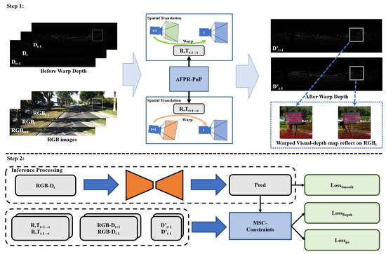
Figure 1.
The framework of the proposed self−supervised depth completion network, step 1: spatial translation for preprocessing; step 2, self−supervised training. Gray rectangles are variables, orange is the inference network, blue is computational modules (no parameters to learn), and green is the loss functions.
This methods is divided into two steps: Step 1, spatial translate the depth map of adjacent frames ( and ) into the current camera field, to generate the and . The pose parameter is provided from AFPR-PnP module. After translation, warped depth points can be reflected on . Step 2, self-supervised training procedure based on multi-modal spatio-temporal consistency (MSC) constraint: It requires a sequence of RGB-D images for training. In the inference processing, it needs only a pair of RGB-D images for generating completion depth.
The pose from the current frame to the adjacent frame is calculated by the PnP algorithm, where . The depth map of adjacent frames ( and ) can be translated to the current camera field ( and ) by and . This is so that a multi-modal spatio-temporal consistency constraint can be built for the self-supervising framework. At the same time, a photometric reproject auto-mask is designed based on the similarity estimation. This automatic mask reduces the displacement errors caused by the depth-temporal point cloud.
The last, an automatic feature points refinement algorithm, is adopted to improve the performance of PnP pose estimation.
This self-supervised framework does not rely on additional sensors, manual tagging efforts, or other learning-based pose estimation algorithms as building blocks. In the inference, only the current frame is needed as an input to generate depth completion.
2.1. Depth-Temporal Consistency Constraint
This paper proposed a self-supervising constraint method based on depth-temporal consistency. The method only needs to obtain synchronous image sequences from monocular cameras and LiDAR. The point clouds of the adjacent frames can be transfered to the current frame to constrain depth completion, as shown in Figure 1-step 1.
As is shown in Figure 2, multi-modal spatio-temporal consistency constraint contains two parts, depth-temporal consistency constraint () and photometric similarity evaluation (PSE). The photometric reproject auto-mask generated by PSE was used to assist the depth-temporal consistency constraint on the current frame.
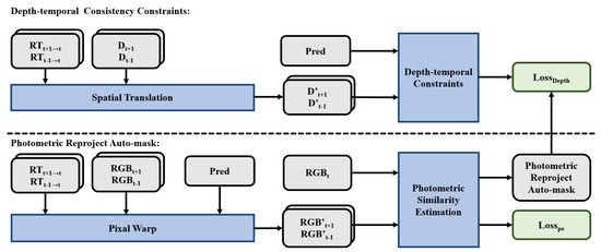
Figure 2.
Multi−modal spatio−temporal consistency constraint.
2.1.1. Spatial Translation
We take at time t, and the adjacent frame as , where . Pose parameters are estimated with and , containing two groups of the rotation matrix and translation (). The detail of pose estimation is introduced in Section 2.3.
The external parameter matrix can be expressed as:
The information of the LiDAR points at time can be transferred to the camera coordinate system at time t through external parameters, and the process can be expressed as:
where . The translated depth map can be calculated by internal parameters:
We can obtain the sparse depth map under the camera coordinate system at the time of t.
2.1.2. Depth-Temporal Consistency Module
Sequential frames contain a lot of spatial structure information. For example, adjacent RGB images have most of the same scenes as the current frame, as do depth images. Different from the point cloud of the current frame (), it provides a lot of depth information in the blank block. However, it cannot be used directly until it is transferred to the current camera field.
The depth-temporal consistency loss function () is built with and . To ground the predictions to a metric scale, we minimize the difference between predictions and the sparse warped depth map and over its domain ( and ):
2.2. Photometric-Temporal Consistency Constraint
Because of the object movement and occlusion, contains many displaced depth points affecting the accuracy of the constraint. Inspired by Godard et al. [33], we select the most similar part of the pixel structure to retain the depth points of this part. The similarity of warped images ( and ) can be used to select the minimum value points in as the automatic photometric reprojection mask ().
We multiply times , and combine their results as a new depth map .
2.2.1. Pixal Warp
Similarly with Section 2.1.1, RGB images will be mapped to the camera coordinate system at t through the pose and predicted depth, as shown in Figure 3.
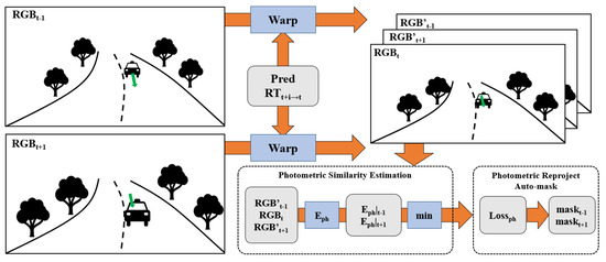
Figure 3.
Warp to with pose () and completion depth (), then generate the automatic photometric reprojection mask.
Take the pixel point of the predicted depth image at , then the pixel point coordinates after the predicted depth can be expressed as:
The sampling function of the warped RGB image at can be expressed as:
Finally, we can obtain the RGB image under the camera coordinate system at the time of t.
2.2.2. Photometric Reproject Auto-Mask
We map the adjacent RGB images to the current RGB image for similarity evaluation by referring to the current predicted depth. The evaluation function contains L1 loss and pixel structure loss.
The photometric error of and can be represented as:
where is the weight between 0 and 1, and the t is time.
We select the adjacent depth point based on the minimum photometric error. Specifically, we took the minimum value of as photometric loss . This photometric loss can overcome the effects of partial occlusion and displacement [33].
It can be expressed as:
and the photometric loss function is:
Among them, generated by selecting the minimum value from and , which means the selected region is the unobstructed part.
The photometric reproject auto-mask according to this characteristics, which represents the most similar part of the warped adjacent RGB images, as shown in Figure 3.
The auto-mask can be represented as:
The auto-mask also represents the most similar part of the depth when it overlaps with the depth image. For the occluded part in a adjacent depth, the auto-mask will have a higher response in another adjacent depth image, to complementing the occluded depth. In the selection of adjacent depths, the auto-mask can provide an available reference. The stitched depth still works on moving objects, unlike photometric errors.
The stitched depth is shown in Figure 4, represented as:
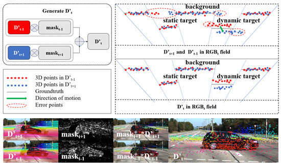
Figure 4.
is generated by splicing high similarity points in (visual process in the bottom). participates in the loss function .
The sequence depth loss function can be represented as:
where is the domain of depth map .
Our multi-modal spatio-temporal consistency constraints include depth-temporal consistency constraint (DC) and photometric-temporal consistency constraint (PC). We implement both constraints with and .
2.3. Automatic Feature Points Refinement
In this method, the stitched depth comes from the translated adjacent depth. The pose estimation network gives constantly adjusted poses, which will bring a heavy calculation to the preprocessing. Therefore, we made the preprocessing dataset with the PnP algorithm, which including the sparse depth after obtaining the fixed pose and translated depth.
Since there are many moving objects in the traffic scene, the feature points from fast-moving objects will affect the estimation in previous PnP algorithms. The automatic feature points refinement proposed as shown in Figure 5, on the left side, the blue point is the matched pair of feature points, the gray point is the camera coordinate system position of feature points (each pair of feature points maps to the same gray point), and the red point is the fast displacement point in the two imaging. On the right side, we line the matched feature points, the green line is the point pair successfully selected, and the red line is the point pair filtered by AFPR-PnP algorithm (the left column is the PnP algorithm designed by Ma, and the right column is ours).

Figure 5.
Automatic feature points’ refinement (AFPR).
Our method adopt the evaluation of moving distance in 3d space to remove interference points. For mismatched points, some of these pairs can be filtered in 2D space, while others are indistinguishable in 2D space, as shown in Figure 5. And such problems can be improved by converting to 3D space coordinate. Assuming that the coordinate of point on the visible image is , and the depth at here is d, the 3D space position can be expressed as :
Transform the feature points into 3D space position coordinates, and calculate their pixel distance and space distance .
We removed the point pairs whose pixel distance exceeded and space coordinate distance exceeded .
3. Experimental Evaluation
3.1. Datasets and Setup
This chapter briefly describes the preprocessing of datasets and design experiments to verify the validity of model.
Datasets: We used KITTI https://www.cvlibs.net/datasets/kitti/raw_data.php (accessed on 21 November 2022) as our data set. In the data pre-processing, we deleted the data of the static scene and the camera on the right. It reduces duplicate scenes and detection points. There are 85,342 training sets. For the test, we selected 1000 test set images for comparison.
Before training, we preprocess the data set. We calculate the Pose parameter through the PnP algorithm, translate the point cloud of the adjacent frame to the current camera coordinate system by parameter, and then splice the translated point cloud according to Formula (11) to generate . Since the PnP algorithm we use is unchanged for each frame, the input results can be reused after saving, thus reducing a lot of training pressure.
Our preprocessing is given in the following Algorithm 1 flow chart:
| Algorithm 1 Data set preprocessing |
|
Setup: We used PyTorch to train the model and cropped the input image to 352*1216. In the pre-processing stage, color correction and noise superposition are performed on the visible light data. We have a learning rate of . Set the batch size to 4, learn 30 epochs, and train the model with an NVIDIA TITAN RTX. We tested the validity of proposed module in three test directions. Our depth completion network adopts the network structure of , and the ResNet18 network experiment verifies the superiority of and PnP algorithms. ResNet34 is used to verify the validity of the deep information mining module. Finally, in comparison with other methods, we also use resnet34.
The final loss function:
where , and are respectively weights of (Function (12)), , and (Function (9)).
During the training, the semi-dense depth labels provided by KITTI were not involved in the calculation. We use the KITTI2012 prediction set https://www.cvlibs.net/datasets/kitti/raw_data.php (accessed on 21 November 2022) and our output results to calculate RMSE error as a standard to evaluate the depth completion accuracy because it is the most representative indicator. RMSE can be expressed as:
denotes the completed depth; denotes the ground-truth depth.
Our training process is given in the following Algorithm 2 flow chart:
| Algorithm 2 Flow chart of self-supervised sequence depth constraint training algorithm. |
|
3.2. Results of the Ablation Experiments
Our multi-modal spatio-temporal consistency (MSC) constraint is embodied in using the consistency of sequence multi-modal information to constrain.
In this section, we compare three self-supervised methods: depth-temporal consistency (DC) constraint, photometric-temporal consistency(PC) constraint, and multi-modal spatio-temporal consistency (MSC) constraint.
As shown in Table 1, the depth completion network can converge smoothly with stitched depth participation in the constraint. As seen in Figure 4, mask comes from the part of the minimum photometric loss, which is multiplied by to filter out most of the wrong displacement points of . This further demonstrates the effectiveness of DC constraints.

Table 1.
Comparison of self-supervised methods for different sequence modality constraints. The bold numbers are the best.
Since RGB and depth data values in different range, and we only regularized RGB images, and the values of and are different from in scale. We tested different values of and . There is much space for optimization in the adjusting parameters.
MSC constraint: As can be observed from Table 1, the MSC method has obvious advantages over single-modal constraint in stable convergence: the lack of any modal constraint ( or ) will crimp the network performance.
- (1)
- Depth-temporal consistency constraint (DC): Many works involve the input depth map in training so that the network will not lose too much depth information. However, due to the displacement between the RGB camera and LiDAR, some of the background depth and the foreground depth are mixed in the same occluded area. Retaining input depth means retaining these erroneous background depth. Our method improved this practice and the stitched sequence depth to replace the current depth.
- (2)
- Photometric-temporal consistency constraint (PC): The sequence depth constraint is too sparse to provide the global constraint. Thus, we introduce the sequence photometric constraint. As shown in the Table 1, the sequence photometric constraint is also indispensable, and the superiority of the sequence multi-modal constraint is also proved. In the DC constraint, this temporal depth data cannot constrain depth completion directly; it contains displaces depth points. This points can affect the performance of depth completion, which was also shown in subsequent experiments. Therefore, we introduce photometric reproject auto-mask to remove these error points, and the experiment proves that this auto-mask is useful.
- (3)
- Multi-modal spatio-temporal consistency constraint (MSC): The MSC constraint contains DC and PC, containing three loss functions. We tested the effect of their weights on the two network structure, S2D [6] and KBNet [31]. As can be observed in the Table 1, the network has the best performance when , , and . We tested several weight ratios of and and finally took , , and as the value of the following experiment.
In addition, we change the input for the experiment, which further verifies that the network can not only mine spatial information but also learn the depth completion from RGB information. As shown in the Table 2, input RGB or Gray images can assist depth completion to generate more accurate depth than input depth only.

Table 2.
Experiment and result comparison of spatial information matching mask. The bold numbers are the best.
AFPR-PnP: In this experiment, we demonstrate the reliability of the PnP algorithm based on automatic feature point refinement. Since S2D [6] have the same pose estimation method (PnP algorithm) with ours. We preprocess the same dataset with the PnP algorithm proposed by Ma et al., train the network in the same way, and compare it with our method. As shown in Figure 5, our PnP algorithm filtered error points, including points on moving cars and different objects with repeating textures.
Specifically, we set , .
As shown in Table 3, we performed ablation experiments with S2D [6] and KBNet [31], the performance for depth completion is enhanced with these methods.

Table 3.
Experiment and result comparison of AFPR-PnP algorithms. The bold numbers are the best.
Discussion: In Figure 6, we compare the performance of model-based depth completion with and without MSC constraint (S2D+MSC(ours) and S2D(Ma)) in detail:
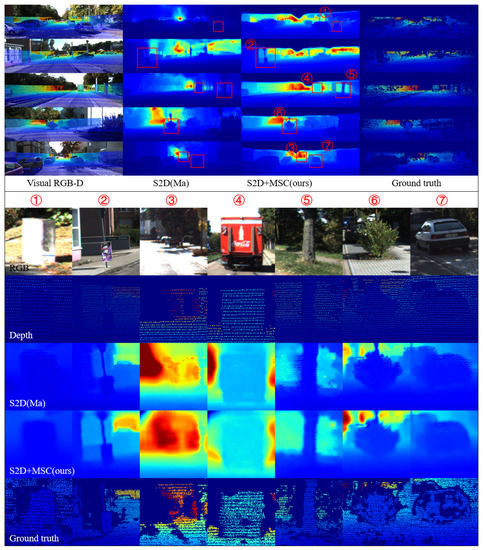
Figure 6.
Results of our self-supervised depth completion on the prediction dataset.
- (1)
- Experiments show that the performance of dark, low-texture parts and distant object is significantly improved(➀ ➁ ➂ ➃).
- (2)
- Sequence depth replaces the input depth as a constraint, so the network does not fully preserve the input depth with its error points. In addition, our photometric similarity estimation module filters out the occlusion points in adjacent depth. Compared with the scheme without MSC constraints, our method reduces the influence of displace points of sparse depth input on depth completion (➄ ➅).
- (3)
- For dynamic targets (➃ ➆), our method has better adaptability.
- (4)
- Our method enhances the fusion ability of the network for multi-modal information, so there will not be a large number of residual sparse points in the image(➀ ➁ ➄ ➅ ➆).
3.3. Results of the Comparative Experiments
As shown in Table 4, we compared the sequence multi-modal constrain self-supervised algorithm with other algorithms on the validation dataset and test set of KITTI2012, and the lower the indicator, the better. We selected DepthComp [5], VOICED [32], SelfDeco [30] and ddp [27] network pose estimation methods to compare with Ma and other PnP pose estimation methods. At the same time, we compare different SLAM acquisition methods. It can be observed that our PnP position estimation method even exceeds the performance of the pose estimation network methods. The stereo images self-supervised method [28] avoids the effect of pose translation with the cost of one more camera, which exceeds the self-supervised scheme of the partial pose estimation network. But our method still has an advantage over it with only a single camera.

Table 4.
The experimental results compared with other methods. The bold numbers are the best.
PnP has the advantages of scene generalization and no training but at the cost of reducing accuracy [5]. However, we still obtain good results with AFPR-PnP algorithm. Additionally, we classify existing constraint methods into multi-modal spatio-temporal consistency constraint (MSC) and photometric-temporal constraint (PC). It can be observed that our MSC constraint method contained DC and PC is more advantageous than only PC.
Discussion: From the comparison (Figure 7) of the output results, our depth completion is better for the interior of the object, while for the edge of the object, our depth completion has fewer wrong completions.
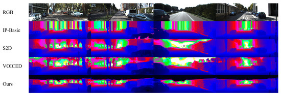
Figure 7.
The results of our self-supervised depth completion compared with others.
By synthesizing all the completion results, it can be observed that the self-supervised completion still has the completion ability for the areas not detected by LiDAR. Compared with the supervised depth completion, it does not rely on manual labelled ground truths and has a better application prospect.
4. Conclusions
To sum up, this paper completed the design of self-supervised depth completion without the ground truth. Among the self-supervised depth completion algorithms, our method is the only one that exploits the MSC constraint. The unique advantage of this method is that it can improve the performance of depth completion on moving objects and occluded/dark light/low texture parts, making the use of the multi-modal spatio-temporal information to the greatest extent. Our experiment demonstrates the effectiveness of our method, even surpassing many supervised methods. However, our method still has much room for improvement. In future work, we will put forward more improvement schemes for the point cloud denoising of sequence LiDAR. Besides, a pose estimation for real-time spatial translation needs to be proposed, and we will focus on improving its estimation accuracy. On this basis, we can still observe the great potential for this kind of self-supervision framework.
Author Contributions
Conceptualization, Q.Z.; Methodology, Q.Z.; Software, Q.Z.; Validation, Q.Z.; Investigation, Q.Z.; Resources, X.C., J.H. and Y.Z.; Writing—original draft, Q.Z.; Writing—review & editing, Q.Z., X.W. and J.Y.; Supervision, X.C., J.H. and Y.Z.; Project administration, X.C.; Funding acquisition, J.H. All authors have read and agreed to the published version of the manuscript.
Funding
This work was supported by National Natural Science Foundation of China (62101256) and China Postdoctoral Science Foundation (2021M691591).
Data Availability Statement
Publicly available datasets were analyzed in this study. This data canbe found here: https://www.cvlibs.net/datasets/kitti/eval_depth.php, accessed on 21 November 2022.
Conflicts of Interest
The authors declare no conflict of interest.
References
- Newcombe, R.A.; Izadi, S.; Hilliges, O.; Molyneaux, D.; Kim, D.; Davison, A.J.; Kohi, P.; Shotton, J.; Hodges, S.; Fitzgibbon, A. Kinectfusion: Real-time dense surface mapping and tracking. In Proceedings of the 2011 10th IEEE International Symposium on Mixed and Augmented Reality, Basel, Switzerland, 26–29 October 2011; pp. 127–136. [Google Scholar]
- Zhang, J.; Singh, S. LOAM: Lidar odometry and mapping in real-time. In Proceedings of the Robotics: Science and Systems, Berkeley, CA, USA, 12–16 July 2014; Volume 2, pp. 1–9. [Google Scholar]
- Li, Y.; Le Bihan, C.; Pourtau, T.; Ristorcelli, T.; Ibanez-Guzman, J. Coarse-to-fine segmentation on lidar point clouds in spherical coordinate and beyond. IEEE Trans. Veh. Technol. 2020, 69, 14588–14601. [Google Scholar] [CrossRef]
- Zhou, H.; Zou, D.; Pei, L.; Ying, R.; Liu, P.; Yu, W. StructSLAM: Visual SLAM with building structure lines. IEEE Trans. Veh. Technol. 2015, 64, 1364–1375. [Google Scholar] [CrossRef]
- Song, Z.; Lu, J.; Yao, Y.; Zhang, J. Self-Supervised Depth Completion From Direct Visual-LiDAR Odometry in Autonomous Driving. IEEE Trans. Intell. Transp. Syst. 2021, 23, 11654–11665. [Google Scholar] [CrossRef]
- Ma, F.; Cavalheiro, G.V.; Karaman, S. Self-supervised sparse-to-dense: Self-supervised depth completion from lidar and monocular camera. In Proceedings of the 2019 International Conference on Robotics and Automation (ICRA), Montreal, QC, Canada, 20–24 May 2019; pp. 3288–3295. [Google Scholar]
- Cui, Y.; Chen, R.; Chu, W.; Chen, L.; Tian, D.; Li, Y.; Cao, D. Deep learning for image and point cloud fusion in autonomous driving: A review. IEEE Trans. Intell. Transp. Syst. 2021, 23, 722–739. [Google Scholar] [CrossRef]
- Uhrig, J.; Schneider, N.; Schneider, L.; Franke, U.; Brox, T.; Geiger, A. Sparsity invariant cnns. In Proceedings of the 2017 International Conference on 3D Vision (3DV), Qingdao, China, 10–12 October 2017; pp. 11–20. [Google Scholar]
- Jaritz, M.; De Charette, R.; Wirbel, E.; Perrotton, X.; Nashashibi, F. Sparse and dense data with cnns: Depth completion and semantic segmentation. In Proceedings of the 2018 International Conference on 3D Vision (3DV), Verona, Italy, 5–8 September 2018; pp. 52–60. [Google Scholar]
- Eldesokey, A.; Felsberg, M.; Khan, F.S. Propagating confidences through cnns for sparse data regression. arXiv 2018, arXiv:1805.11913. [Google Scholar]
- Eldesokey, A.; Felsberg, M.; Khan, F.S. Confidence propagation through cnns for guided sparse depth regression. IEEE Trans. Pattern Anal. Mach. Intell. 2019, 42, 2423–2436. [Google Scholar] [CrossRef] [PubMed]
- Yan, L.; Liu, K.; Belyaev, E. Revisiting sparsity invariant convolution: A network for image guided depth completion. IEEE Access 2020, 8, 126323–126332. [Google Scholar] [CrossRef]
- Huang, Z.; Fan, J.; Cheng, S.; Yi, S.; Wang, X.; Li, H. Hms-net: Hierarchical multi-scale sparsity-invariant network for sparse depth completion. IEEE Trans. Image Process. 2019, 29, 3429–3441. [Google Scholar] [CrossRef] [PubMed]
- Ma, F.; Karaman, S. Sparse-to-dense: Depth prediction from sparse depth samples and a single image. In Proceedings of the 2018 IEEE International Conference on Robotics and Automation (ICRA), Brisbane, QLD, Australia, 21–25 May 2018; pp. 4796–4803. [Google Scholar]
- He, K.; Zhang, X.; Ren, S.; Sun, J. Deep residual learning for image recognition. In Proceedings of the IEEE Conference on Computer Vision and Pattern Recognition, Las Vegas, NV, USA, 27–30 June 2016; pp. 770–778. [Google Scholar]
- Wei, M.; Zhu, M.; Zhang, Y.; Sun, J.; Wang, J. An Efficient Information-Reinforced Lidar Deep Completion Network without RGB Guided. Remote. Sens. 2022, 14, 4689. [Google Scholar] [CrossRef]
- Hu, M.; Wang, S.; Li, B.; Ning, S.; Fan, L.; Gong, X. Penet: Towards precise and efficient image guided depth completion. In Proceedings of the 2021 IEEE International Conference on Robotics and Automation (ICRA), Xi’an, China, 30 May–5 June 2021; pp. 13656–13662. [Google Scholar]
- Li, A.; Yuan, Z.; Ling, Y.; Chi, W.; Zhang, C. A multi-scale guided cascade hourglass network for depth completion. In Proceedings of the IEEE/CVF Winter Conference on Applications of Computer Vision, Snowmass, CO, USA, 1–5 March 2020; pp. 32–40. [Google Scholar]
- Liu, L.; Song, X.; Lyu, X.; Diao, J.; Wang, M.; Liu, Y.; Zhang, L. FCFR-Net: Feature fusion based coarse-to-fine residual learning for depth completion. arXiv 2020, arXiv:2012.08270. [Google Scholar] [CrossRef]
- Zhang, Y.; Funkhouser, T. Deep depth completion of a single rgb-d image. In Proceedings of the IEEE Conference on Computer Vision and Pattern Recognition, Salt Lake City, UT, USA, 18–23 June 2018; pp. 175–185. [Google Scholar]
- Qiu, J.; Cui, Z.; Zhang, Y.; Zhang, X.; Liu, S.; Zeng, B.; Pollefeys, M. Deeplidar: Deep surface normal guided depth prediction for outdoor scene from sparse lidar data and single color image. In Proceedings of the IEEE/CVF Conference on Computer Vision and Pattern Recognition, Long Beach, CA, USA, 15–20 June 2019; pp. 3313–3322. [Google Scholar]
- Xu, Y.; Zhu, X.; Shi, J.; Zhang, G.; Bao, H.; Li, H. Depth completion from sparse lidar data with depth-normal constraints. In Proceedings of the IEEE/CVF International Conference on Computer Vision, Seoul, Republic of Korea, 27 October–2 November 2019; pp. 2811–2820. [Google Scholar]
- Nazir, D.; Liwicki, M.; Stricker, D.; Afzal, M.Z. SemAttNet: Towards Attention-based Semantic Aware Guided Depth Completion. arXiv 2022, arXiv:2204.13635. [Google Scholar] [CrossRef]
- Yue, J.; Wen, W.; Han, J.; Hsu, L.T. 3D Point Clouds Data Super Resolution-Aided LiDAR Odometry for Vehicular Positioning in Urban Canyons. IEEE Trans. Veh. Technol. 2021, 70, 4098–4112. [Google Scholar] [CrossRef]
- Cheng, X.; Wang, P.; Yang, R. Learning depth with convolutional spatial propagation network. IEEE Trans. Pattern Anal. Mach. Intell. 2019, 42, 2361–2379. [Google Scholar] [CrossRef] [PubMed]
- Cheng, X.; Wang, P.; Guan, C.; Yang, R. Cspn++: Learning context and resource aware convolutional spatial propagation networks for depth completion. In Proceedings of the AAAI Conference on Artificial Intelligence, New York, NY, USA, 7–12 February 2020; Volume 34, pp. 10615–10622. [Google Scholar]
- Yang, Y.; Wong, A.; Soatto, S. Dense depth posterior (ddp) from single image and sparse range. In Proceedings of the IEEE/CVF Conference on Computer Vision and Pattern Recognition, Long Beach, CA, USA, 15–20 June 2019; pp. 3353–3362. [Google Scholar]
- Shivakumar, S.S.; Nguyen, T.; Miller, I.D.; Chen, S.W.; Kumar, V.; Taylor, C.J. Dfusenet: Deep fusion of rgb and sparse depth information for image guided dense depth completion. In Proceedings of the 2019 IEEE Intelligent Transportation Systems Conference (ITSC), Long Beach, CA, USA, 15–20 June 2019; pp. 13–20. [Google Scholar]
- Feng, Z.; Jing, L.; Yin, P.; Tian, Y.; Li, B. Advancing self-supervised monocular depth learning with sparse liDAR. In Proceedings of the Conference on Robot Learning, Auckland, New Zealand, 14–18 December 2022; pp. 685–694. [Google Scholar]
- Choi, J.; Jung, D.; Lee, Y.; Kim, D.; Manocha, D.; Lee, D. Selfdeco: Self-supervised monocular depth completion in challenging indoor environments. In Proceedings of the 2021 IEEE International Conference on Robotics and Automation (ICRA), Xi’an, China, 30 May–5 June 2021; pp. 467–474. [Google Scholar]
- Wong, A.; Soatto, S. Unsupervised depth completion with calibrated backprojection layers. In Proceedings of the IEEE/CVF International Conference on Computer Vision, Montreal, QC, Canada, 10–17 October 2021; pp. 12747–12756. [Google Scholar]
- Wong, A.; Fei, X.; Tsuei, S.; Soatto, S. Unsupervised depth completion from visual inertial odometry. IEEE Robot. Autom. Lett. 2020, 5, 1899–1906. [Google Scholar] [CrossRef]
- Godard, C.; Mac Aodha, O.; Firman, M.; Brostow, G.J. Digging into self-supervised monocular depth estimation. In Proceedings of the IEEE/CVF International Conference on Computer Vision, Seoul, Republic of Korea, 27 October–2 November 2019; pp. 3828–3838. [Google Scholar]
- Ku, J.; Harakeh, A.; Waslander, S.L. In defense of classical image processing: Fast depth completion on the cpu. In Proceedings of the 2018 15th Conference on Computer and Robot Vision (CRV), Toronto, ON, Canada, 8–10 May 2018; pp. 16–22. [Google Scholar]
Disclaimer/Publisher’s Note: The statements, opinions and data contained in all publications are solely those of the individual author(s) and contributor(s) and not of MDPI and/or the editor(s). MDPI and/or the editor(s) disclaim responsibility for any injury to people or property resulting from any ideas, methods, instructions or products referred to in the content. |
© 2022 by the authors. Licensee MDPI, Basel, Switzerland. This article is an open access article distributed under the terms and conditions of the Creative Commons Attribution (CC BY) license (https://creativecommons.org/licenses/by/4.0/).