Article

Enhancing Solar Energy Forecast Using Multi-Column Convolutional Neural Network and Multipoint Time Series Approach

by
Anil Kumar
1,
Yashwant Kashyap
1,* and
Panagiotis Kosmopoulos
2,*
1
Electrical and Electronics Engineering Department, National Institute of Technology Karnataka, Surathkal 575025, India
2
Institute for Environmental Research and Sustainable Development, National Observatory of Athens (IERSD/NOA), 15236 Athens, Greece
*
Authors to whom correspondence should be addressed.
Remote Sens. 2023, 15(1), 107; https://doi.org/10.3390/rs15010107
Submission received: 2 October 2022 / Revised: 13 December 2022 / Accepted: 20 December 2022 / Published: 25 December 2022
(This article belongs to the Special Issue Remote Sensing in Environmental Modelling)

Abstract

:
The rapid expansion of solar industries presents unknown technological challenges. A dedicated and suitable energy forecast is an effective solution for the daily dispatching and production of the electricity grid. The traditional forecast technique uses weather and plant parameters as the model information. Nevertheless, these are insufficient to consider problematic weather variability and the various plant characteristics in the actual field. Considering the above facts and inspired by the excellent implementation of the multi-column convolutional neural network (MCNN) in image processing, we developed a novel approach for forecasting solar energy by transforming multipoint time series (MT) into images for the MCNN to examine. We first processed the data to convert the time series solar energy into image matrices. We observed that the MCNN showed a preeminent response under a ground-based high-resolution spatial–temporal image matrix with a 0.2826% and 0.5826% RMSE for 15 min-ahead forecast under clear (CR) and cloudy (CD) conditions, respectively. Our process was performed on the MATLAB deep learning platform and tested on CR and CD solar energy conditions. The excellent execution of the suggested technique was compared with state-of-the-art deep neural network solar forecasting techniques.

1. Introduction

Over several years, the main objective of global sustainable development and mitigation policies for climate change has been to focus on renewable against coal energy production. The energy crisis and environmental issues are being raised all over the world. Photovoltaic (PV) production has grown fast due to wide applications in clean energy [1]. According to the International Renewable Energy Agency (IRENA) statistics, the worldwide deployed potential exceeded 580 GW in 2019 [2]. The output of solar PV generation and solar thermal power stations or photovoltaic/thermal (PV/T) reservoir systems [3] depends on various factors such as solar irradiance, temperature, climate, and other factors [4]. The prediction of solar irradiance plays a significant role in the security of the power grid [5]. Several models have been developed by experts for the prediction of global horizontal irradiance (GHI), which are classified under six categories as follows: persistence models, classical statistical models, machine learning methods, cloud motion tracking methods, numerical weather prediction models (NWP), and hybrid models [6]. In persistence models, the solar irradiance measurement at time T is equal to that at time T-1. During the last few years, persistence models have been used to compare the improvements in the performance of other models. The most popular method for predicting solar irradiance is climatology-persistence (Clim-Pers) [7]. The classical statistical models establish the relation between the parameters obtained through the dataset’s statistical analysis. Such models are as follows: Markov processes, regression, exponential smoothing models, autoregressive (AR) models, autoregressive moving average (ARMA) models, and autoregressive integrated moving average (ARIMA) models [8]. One of the demerits of statistical models is that they cannot tackle instantly varying non-static data. The prediction accuracy for the sudden change in the non-static data of solar irradiance is low. A machine-learning-based model can learn and design the complex non-linear relationship using the solar irradiance data and meteorological parameters. Artificial neural networks (ANNs), support vector machine (SVM), extreme learning machine (ELM), the genetic algorithm (GA), the hidden Markov model (HMM), naive Bayes, the Gaussian process (GP), the k-means clustering algorithm, and decision trees (DTs) were formulated for irradiance prediction [9,10,11]. Caldas and Alonso-Suarez, Peng et al., and Chu et al. reported that various algorithms are utilized for cloud motion tracking to predict the irradiances by the all-sky imagers or satellites. ANN-based GHI prediction is assessed using satellite images, where the cloud fraction is used as the input, obtained from satellite image processing [12]. In order to simulate the physical system in atmospheric transformation and forecast weather, the current weather mathematical model is utilized in the NWP method [13,14,15]. In [16,17,18], the authors utilized the NWP model and related technology to predict the solar irradiance. The hybrid models are widely used as they combine other methods’ advantages. Currently, many hybrid models have been developed to predict solar irradiance. In [19], Ji and Chee developed a hybrid model consisting of the ARMA model and the controversial time-delay neural network (TDNN) for hourly solar energy forecasting. ARMA and the TDNN show good accuracy, where ARMA is designed for the prediction of linear components of time series and the TDNN is also used to predict the solar irradiance. In [20], the HMM and generalized fuzzy model (GFM) were utilized for solar forecasting. Unsupervised clustering is used in the HMM method, and GFM has been applied to fine-tune the clustering for a desirable accuracy of solar radiation prediction. In [21], Voyant et al. developed a model that combines ANN and ARMA for an hourly forecast of global horizontal irradiance. The ANN is utilized for cloudy conditions, and ARMA is utilized on sunny days. In [22], Dong et al. formulated a new hybrid framework that combines the exponential smoothing state space (ESSS) and the ANN for predicting GHI from satellite images. The ESSS was used to predict the cloud cover index, and solar irradiance estimation depending on the cloud cover index was performed utilizing the ANN. In [23], a hybrid framework was developed, which was the combination of self-organizing maps (SOMs), SVR, and the particle swarm optimization (PSO) technique. Several disorganized regions were created corresponding to all the inputs utilizing the SOMs, then SVR and PSO were utilized to frame each disjointed region to predict the output. A hybrid model was developed, which combined fuzzy regression functions (FRFs) and SVM in order to predict horizontal global solar radiation [24].
Some other hybrid models have been developed for the prediction of solar radiation, which are based on different data preprocessing methods such as the wavelet transform (WT), wavelet decomposition (WD), wavelet packet decomposition (WPD), empirical mode decomposition (EMD), ensemble empirical mode decomposition (EEMD), complete ensemble empirical mode decomposition-adaptive noise (CEEM-DAN), principal component analysis, etc.
Mohammadi et al. [25] and Deo et al. [26] developed a hybrid model where SVMs and the WT algorithm were combined together for the prediction of GHI. Wavelet analysis was utilized to decompose time series into various sub-time series. These sub-time series were utilized as the input for the SVMs to complete the GHI prediction. In [27], Hussian and A.I. Alili proposed a hybrid model, which combines WD with the ANN for the decomposition of complex meteorological signals into simple sub-time series. Then, these sub-time series were modeled using the ANN, and the output was reconstructed to predict GHI. In [28], Lan et al. proposed a novel method consisting of the EEMD-SOM-BP method. EEMD was utilized to decompose the original data into sub-time series with different frequencies. These sub-time-series were used as the input to the SOM-BP networks. The output of each SOM-BP network is the predicted output of the solar radiance. This output is the algebraic sum of each SOM-BP network. In [29], Davo et al. introduced a hybrid model, which was the combination of principal component analysis (PCA) with the ANN and the analog ensemble (AnEn) for the prediction of solar radiance and wind power. The main objective of PCA was to reduce the dimension of the NWP data, whereas the ANN and AnEn were used to train and forecast solar radiances. In [30], the data were decomposed using WPD, and a new deep-learning-based hybrid model was developed in which WPD was combined with LSTM for PV power prediction. In [31], a CNN, LSTM, and CNN-LSTM comparison was given for 60 min-ahead PV power prediction for different seasons using the historical PV power. Rami Al-Hajj [32] leveraged the advantages of the multi-level stacking of LSTM and MLP for day-ahead solar radiation forecasting. The CNN, LSTM, and its derivatives were developed for solar PV power forecast using ground and satellite data. The innovations of this study are given as follows:
  • We propose the Gramian cloud field (GCF) matrix (Section 2.1.1) to understand the clouds’ impact on solar power generation from ground-measured spatial and temporal solar power components.
  • We evaluated the performance of the proposed models in different domains, namely time series, temporal, spatial, and spatial–temporal.
  • For the first time, the CNN was used to forecast solar PV power using the multipoint and GCF approaches.
  • We designed the MCNN model for use with multi-resolution input images from satellite and ground data. However, the target was the ground (in situ) data only.
The following Section 2.1 describes the data processing and the filling of the missing values involved in the model. Section 2.1.1 describes the time series-to-image matrix conversion approach. Section 2.2 gives the DNN framework of the two network structures for the present model. Section 2.3 describes the training of the DNN for the present model, which consists of the model setup in Section 2.3.1, the settings in Section 2.3.2, and the performance in Section 2.3.3. The results are discussed in Section 3, which include a comparison of the models in Section 3.1, the effect of the MCNN in Section 3.2, the effect of clear–cloudy conditions in Section 3.3, and the effect of the satellite inputs in Section 3.4 for the model validation. The conclusions of this research work are described in the last Section 4.

2. Methodology

2.1. Data Processing

Solar PV energy depends on multiple factors, primarily geographic location and atmospheric conditions. These factors were further classified into and analyzed as spatial and temporal distributions. The spatial analysis consisted of plant size, weather phenomena, panel distribution, panel orientation, facing direction, Sun tracing, etc. Furthermore, the temporal analysis depends on weather disturbance and the seasons, months, days, and hours of the years [33]. The careful investigation of these spatial and temporal data can enhance the accuracy of the prediction [34]. We included solar irradiance and power generation data to forecast 2 h solar energy production. The collected raw dataset contains solar irradiance and the power generation time series from 00:00H, 1 March 2020, to 24:00H, 31 March 2021, from Southern India. The solar power generation consists of spatial and temporal components at 5 min intervals and 22 random locations of the plants, as depicted in Figure 1. Figure 1 is the general layout of the studied solar farm to show the sub-distribution of the panels and data collection regions. Our plant capacity is 80 MW, consists of 2.5 million modules, and covers an area of almost 1.2 km2. Our aim was to elaborate the plant for better accuracy. Of course, we can increase the number of observation points, as well as the plants, but we had limitations. The units for solar energy are presented in kWh and MWh. The Gramian cloud field (GCF) matrix [35] is proposed to convert solar temporal series to spatial image matrices, which comprised the input data framework of the DNN model.

2.1.1. GCF Matrix

The Gram matrix (GM) is commonly used to evaluate the linear dependence of a set of vectors. The Gram matrix is defined in Equation (1) for a given set of vectors [35]. The Gram matrix was formulated by the use of actual time series data to create Figure 2b, and the spatial data were used to create Figure 2c.
G M = < x 1 , x 1 > < x 1 , x m > < x n , x 1 > < x n , x m >
where < > is the inner product of the two matrices.
Inspired by the Gram matrix, we suggest the Gramian cloud field (GCF) matrix [36]. Here, to understand the clouds’ impact on solar power generation from the ground-measured parameters given in time series u 1 , u 2 , u n and spatial data v 1 , v 2 , v n , the solar components provide the movements of the clouds. The cloud movements can be divided into two components for the ease of calculation. The first determines the cloud direction D C i and, the second, an approximation of the cloud potential C P i from multiple coordinates at every 5 min by Equation (2):
D C i = arctan u i v i ; C P i = · 5 × u i 2 + v i 2
After rescaling cloud potential component CP to [0, 1] by min–max normalization, we built a vector, C = c 1 , c 2 c n , which contains cloud features c i , in the polar coordinate system C P i , D C i . The elements of vector c i are cloud features that contain the normalized value of DC and CP. The min–max normalization was obtained using Equation (3) to improve the computational speed and accelerate the network’s training convergence speed [37].
C P i = C P C P m i n C P m a x C P m i n
where C P i is the data after the min–max normalization of the original data (CP). C P m a x and C P m i n are the maximum and minimum value of the original data. The GCF matrix formulation is explained in Equation (4):
G C F = < w 1 , w 1 > < w 1 , w m > < w n , w 1 > < w n , w m >
where < w 1 , w 2 > is inner product between w 1 and w 2 :
< w 1 , w 2 > = C P 1 cos D C 1 × C P 2 cos D C 2 + C P 1 sin D C 1 × C P 2 sin D C 2
Every timestamp (i) of the time series (TS) data is represented as vector w i in the polar coordinate system ( C P i , D C i ). Diagonal elements characterize the features of the cloud correlation vectors at each timestamp. In comparison, the other elements represent the cross-co-relationship between cloud vectors at different timestamps. In the raw dataset, there were twenty-two TSs from different locations, which were mapped to five-channel images, as shown in Figure 2b–f.
Regarding the GCF image matrix conversion, the matrix’s row and column are the 22 locations (every 5 min) of solar power in the space and time domains. Therefore, n and m in the GCF matrix represent the 22 locations. An example of the GCF image formation based on the available spatial–temporal solar data is shown in Figure 2a; the spatial distributions of the normalized solar power of the 22 locations are shown in the bottom x-axis (space label) versus solar power in the left y-axis, similar to the time domain distribution of the previous 22 values ( t 1 , t 2 , t 22 ) shown in the top x-axis (time label) versus solar power in the right y-axis. In Figure 2a, the spatial data (red line) illustrate the values of a certain point in time, and temporal data (black line) are for a certain location. The image in Figure 2b,c is derived from the GM in Equation (1). The GCF image matrix is derived from Equation (4), and the proposed combination of multiple space and time correlation matrices is shown in Figure 2d–f to understand the solar power distribution properly in the time and space domains. Figure 2b is an image of the temporal distribution of Figure 2a (black color) of the solar power of the 22 previous temporal values derived from the GM in Equation (1). The row (n) and column (m) of Figure 2b are the time vectors. Figure 2c is also derived from the GM in Equation (1), which is based on the spatial distribution of the solar power at the 22 locations, shown in Figure 2a in red color. The row and column of Figure 2c are the space vectors. The GCF images in Figure 2d,e were derived from Equation (4), keeping the time and space domain values, respectively. Figure 2f represents the spatiotemporal image from Equation (4) of the 22 points’ space and time distributions.
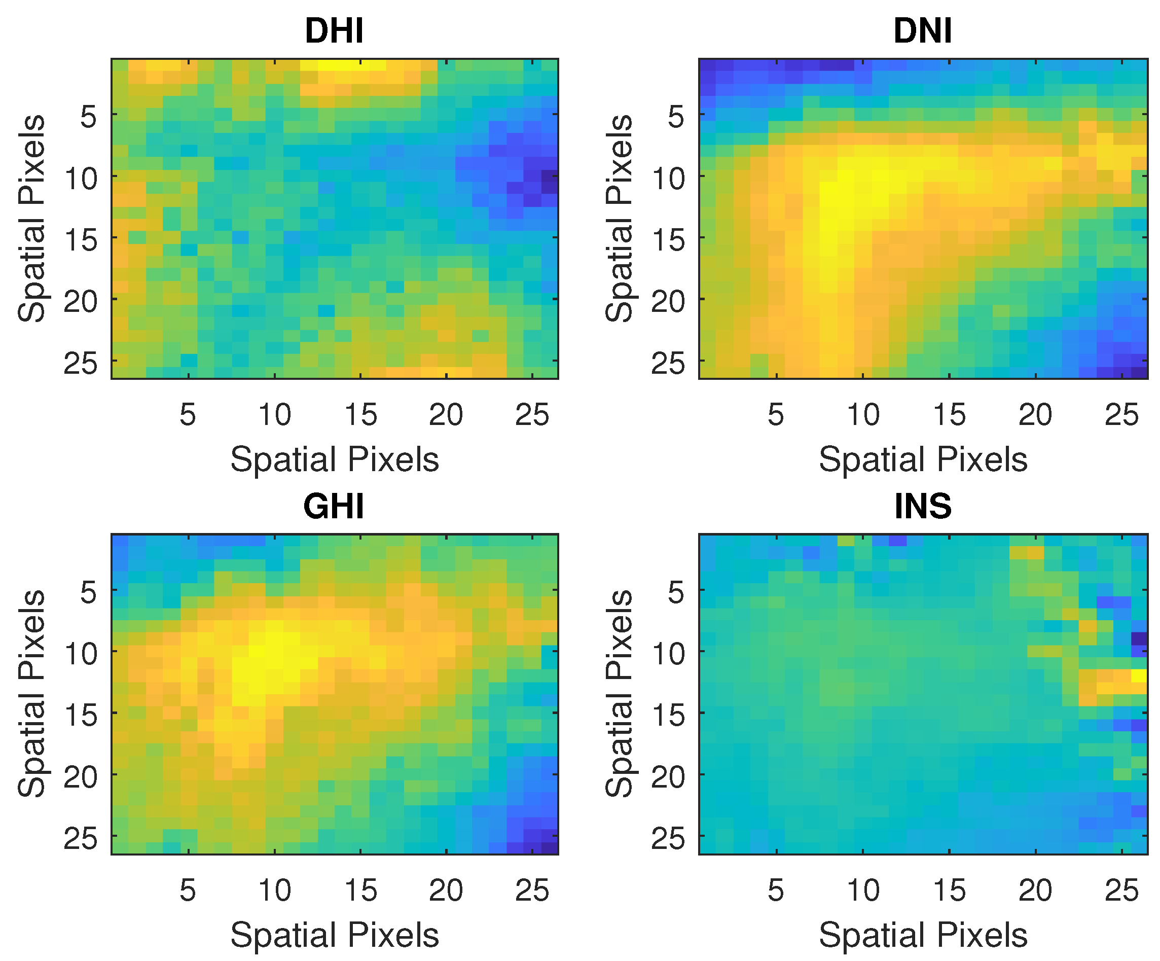
The satellite irradiance components diffuse horizontal irradiance (DHI), direct normal irradiance (DNI), global horizontal irradiance (GHI), and insolation (INS) were considered for the further analysis and verification of the solar power generation at the plant location, as shown in Figure 3.
The satellite data’s 4 km spatial and 15 min temporal resolution were different from the ground-measured data, requiring transforming the GCF images. The satellite images benefited the cloud movement tracking for the large-scale spatial analysis. Therefore, the spatial distribution of the image size was considered as 100 × 100 km, which is 30-times larger than the actual plant size. The Sun’s movement was considered better with a larger satellite image, around the clock. The cloud shadow variation calculated over the plants was based on the clouds’ altitude (roughly 8 to 20 km) with respect to the horizontal and vertical movements in the sky. In the present study, we used the radiative transfer model (RTM) simulations produced by libRadtran [38,39] to estimate the solar irradiance. A fast version of RTM was developed by [40] based on pre-calculated look-up tables and a replicate for India by [41]. The major input parameters for the RTM simulations are the aerosol and cloud optical properties, the solar elevation and orientation, the total ozone column, and the columnar water vapor. The outputs of the RTM simulation are the DHI, DNI, GHI, and INS, which cover the wavelength range from 285 to 2700 nm and use the SBDART radiative transfer solver [42] with the pseudo-spherical approximation to generate the valid output for solar elevations between 0 and 90 degrees. The model simulation was performed using the band parameterization method based on the correlated-K approximation [43], along with aerosol and cloud determination, which were performed based on the default available aerosol models [44].

2.2. Deep Neural Network Structure

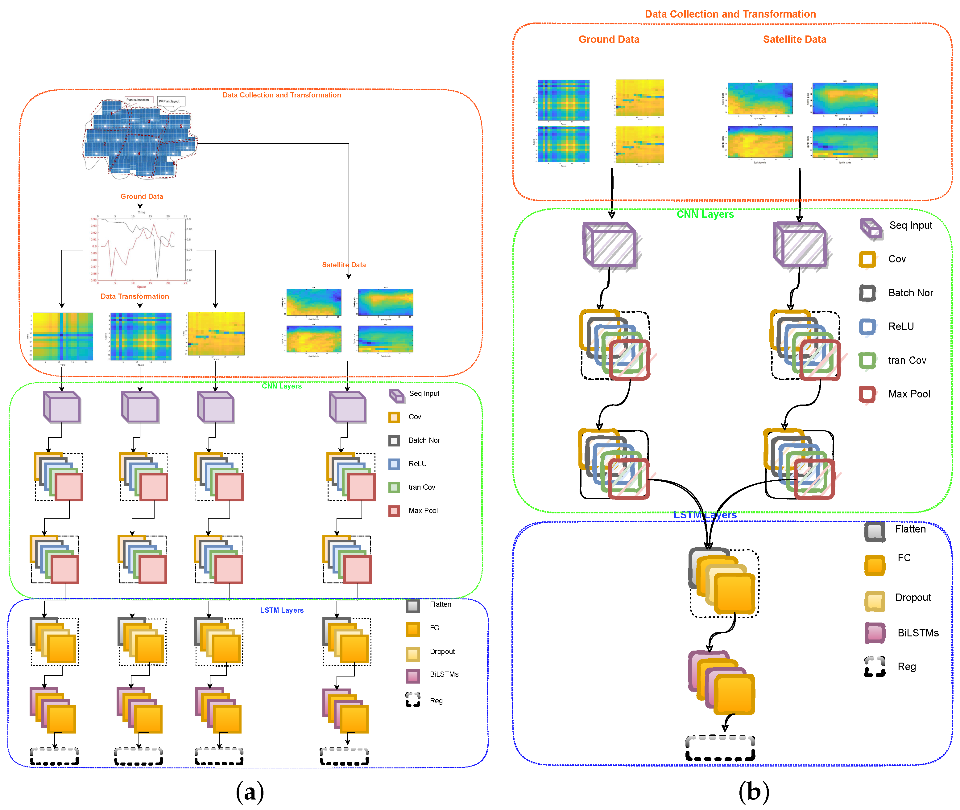
The TS-to-image matrix conversion using the GCF algorithm in Equation (4), the available twenty-two 1 D images, five 2 D single-channel sequential images’ spatiotemporal mapping, and one 3 D four-channel satellite image formed the solar irradiance dataset used for the study. The comparison was performed using the popular convolutional neural network (CNN) [45], long short-term memory (LSTM) [46], a combination of both (CNN-LSTM) [47], and the MCNN [48] to retrieve the features from the above matrices and the output of a 2 h solar power forecast, as shown in Figure 4, showing the complete model network structure. From Figure 4, Seq, Cov, Batch Nor, Tran Cov, Max Pool, F.C., and Reg denote the sequence, convolution, batch normalization, transposed convolution, max pooling, fully connected, and regression layers, respectively. The sequence input layer features are defined as per the input data types 1 × 1 , 22 × 1 , 22 × 22 × 1 , 22 × 22 × 5 , and 26 × 26 × 4 for single-input time series, multiple-input time series, 2D images with five channels, and 3D images with four channels for the input dimensions, respectively [49]. The filters and convolution kernel size started from 8@ 3 × 3 for the first, 16@ 3 × 3 for the second, etc., as depicted in Figure 4. In the present study, in the CNN model, a five-times Cov layer was used, with a maximum filter size of 72@ 3 × 3 . Each Cov layer consisted of a stride of one and zero padding.
We used the Tran Cov layer for upsampling [50]. The Tran Cov layer creates an output feature map with a greater spatial dimension than the input, making the regression more robust. To avoid the overfitting problem and speed up the training procedure, we used a dropout layer (the dropout rate was 0.25) [51], a batch normalization layer, max pooling, to help extract low-level features, and ReLU, to avoid the vanishing gradient problem, which has a much lower runtime [52]. We used the BiLSTM layer [53,54] following the convolutional layer. The BiLSTM layer can control the bidirectional dependencies passed on in the sequence data at every step. The fully connected layer starts from 484, 242, 121, 60, and 22 units to the final regression layer. In order to prevent potential interferences, we merged the two networks (CNN and LSTM) and connected the final forecast layer to another fully connected layer. We used two spatial image sources, one the ground and the other the satellite image, with different spatial resolutions, to overcome the different spatial resolution problems using multi-stream CNN, multi-input CNN, or multi-column CNN-LSTM (MCCN) [48], as shown in Figure 4b.

2.3. DNN Properties

Once having processed the data (Section 2.1 and Section 2.1.1) and created the model network structure (Section 2.2), the next step was the model properties’ definition. This is divided into the following sub-sections:
Section 2.3.1: DNN Setup;
Section 2.3.2: DNN Settings;
Section 2.3.3: DNN Performance Parameters.

2.3.1. DNN setup

The whole dataset consisted of 22 TS data points, and each TS contained 1,03,680 points for every 5 min of solar power generation from March 2020 to 2021. Each TS point was considered an independent case, and we divided the 1,03,680-sample dataset into training and testing sets with a 7:3 ratio. Finally, we trained and tested the whole dataset using the deep learning toolbox from MATLAB 2021b for data processing, network design, and training using a GPU.

2.3.2. DNN Settings

Three popular time series forecasting methods for all possible input datasets were tested to demonstrate and analyze the proposed hybrid method. The proposed well-known methods were CNN-LSTM [47], LSTM [46], and CNN [45], taken for the comparison and assessments. The input data types were kept the same: 1D, 2D, and 3D, to assess the three network structures uniformly. The basic model settings and parameters are listed in Table 1.

2.3.3. DNN Performance Parameters

The model performance was evaluated based on the root-mean-squared error (RMSE) and mean absolute error (MAE) metrics for the purposes of comparison, which are formulated as below:
RMSE method: This method evaluates the standard deviations in the predicted solar power, calculated by using the equation:
R M S E Y T = i = 1 N ( y a c t u a l y p r e d i c t ) 2 N
where R M S E Y T denotes the RMSE of solar power, y a c t u a l is the solar power from the field test, y p r e d i c t is the predicted solar power from the machine learning algorithm, and N is the number of non-missing data points.
MAE method: This method calculates the mean absolute error involved in solar power measurement. The absolute error is the difference between the actual and predicted one. The formula to calculate the MAE for power is given below:
M A E Y T = i = 1 N | y a c t u a l y p r e d i c t | N
where M A E Y T is the mean absolute error of the power and N is the number of errors.
The assessment consisted of four major domains, namely time series, temporal, spatial, and spatiotemporal, to understand the response of the predefined methods as mentioned in Table 2:
1
The validation of the proposed approach was performed by comparing with single and multiple inputs to match the single and multiple outputs on a typical time series dataset.
2
The validation of the proposed approach is illustrated to reveal the effectiveness of the 2D input image metrics in the spatial domain to match the single and multiple outputs on a typical time series dataset.
3
Similarly, the validation of the proposed approach is illustrated to reveal the effectiveness of the 2D input image metrics in the temporal domain to match the single and multiple outputs on a typical time series dataset.
4
Finally, the validation of the proposed approach is illustrated to reveal the effectiveness of the 2D input image metrics in the spatiotemporal domain to match the single and multiple outputs on a typical time series dataset.
Table 2. Experiment settings and parameters.
NameDIUnitTypeSourcesCategoryLayersM-TypeOutputs
M11DMWTsGDCR+CD2LSTM1
M21DkWTsGDCR+CD2LSTM1
M31DkWTsGDCR+CD2LSTM22
M42DkWSpGDCR+CD2CNN1
M52DkWSpGDCR+CD2CNN22
M62DkWTpGDCR+CD2CNN1
M72DkWTpGDCR+CD2CNN22
M82DkWSp-TpGDCR+CD2CNN1
M92DkWSp-TpGDCR+CD2CNN22
M101DkWSp-Tp VGDCR+CD2LSTM1
M111DkWSp-Tp VGDCR+CD2LSTM22
M122DkWSpGDCR+CD4CNN-LSTM1
M132DkWSpGDCR+CD4CNN-LSTM22
M142DMWTpGDCR+CD4CNN-LSTM1
M152DkWTpGDCR+CD4CNN-LSTM22
M162DkWSp-TpGDCR+CD4CNN-LSTM1
M172DkWSp-TpGDCR+CD4CNN-LSTM22
M182DkWSp-TpGDCR4CNN-LSTM22
M192DkWSp-TpGDCD4CNN-LSTM22
M202DkWSp-TpSatCR4CNN-LSTM22
M212DkWSp-TpSatCD4CNN-LSTM22
M222DkWSp-TpSat+GDCR4CNN-LSTM22
M232DkWSp-TpSat+GDCD4CNN-LSTM22
M242DkWSp-TpGDCR4MCNN22
M252DkWSp-TpGDCD4MCNN22
M262DkWSp-TpSatCR4MCNN22
M272DkWSp-TpSatCD4MCNN22
M282DkWSp-TpSat+GDCR4MCNN22
M292DkWSp-TpSat+GDCD4MCNN22

3. Experimental Results and Evaluation

Once having processed the data (Section 2.1 and Section 2.1.1), created the model network structure (Section 2.2), and defined the model properties (Section 2.3), the next step was the evaluation process. This is divided into the following sub-sections:
Section 3.1: Comparison of Methods;
Section 3.2: Effects of Multi-Column CNN-LSTM Model;
Section 3.3: Effects of Cloudy Conditions;
Section 3.4: Effects of Satellite Inputs.

3.1. Comparisons of Methods

To evaluate the performance of the proposed method, we compared the performance of different methods in the following time steps in minutes: 5, 10, 15, 20, 25, 30, 35, 40, 45, 50, 55, 60, 65, 70, 75, 80, 85, 90, 95, 100, 105, 100, 115, 120. The results of the twenty-two locations were combined and presented in Figure 5 and Figure 6, and the detailed MAE and RMSE results are given in Table 3. Moreover, we provide the detailed MAE and RMSE comparison results for the twenty-two locations under the 90 and 15 min time steps in Figure 7 and Figure 8, respectively. In addition, we introduce the MCNN to combine the ground and satellite images in Figure 9. Further, we introduced the clear and cloudy day effect on the model’s performance, as shown in Figure 10 and Figure 11, respectively, at 15 min time steps. We finally introduce the satellite spatial information compared to the ground database, as shown in Figure 12.
Table 3 presents the detailed MAE and RMSE comparison of all 29 models at multiple time steps (15, 30, and 90 min). We compared the few models that performed well, such as M7, M15, and M17, based on the ground image inputs under clear–cloudy circumstances. For further analysis of the model performance, we tested the models [M18-M29] based on the ground (GD), satellite (Sat), and satellite–ground (Sat-GD) combined inputs under the consideration of clear and cloudy situations separately. Among all these models, M18, M19, M24, and M25 showed excellent performance for all time steps. Above all, [M15,M17], [M18,24], and [M19, M25] performed well for multiple time steps based on the GD approach under the CR-CD, CR, and CD conditions, respectively. Further, the multiple input and output model’s results were constantly improved in comparison to the single input–output model [55,56].
Figure 5 shows the performance of the single versus multiple points approach for 2 h-ahead forecast in time steps of 5 min. Shown in Figure 5a,b are single versus multiple inputs and in Figure 5c,d single versus multiple outputs. The multipoint approach outperformed the single-point approach for all time steps. The multiple point approach offered 29.2060% and 36.5758% reductions in the MAE and 41.6292%, and 56.4366% reductions in the RMSE compared to the single-point approach. Notably, the multipoint approach had better performance between 1–9 and 8–21 time steps for the multiple input (M2) and multiple output (M3) approach, respectively.
Figure 6 shows the CNN and combined model (CNN-LSTM) approaches with spatial, temporal, and spatiotemporal as the input conditions and witnesses the MAE and RMSE decline for the spatiotemporal approach. However, the CNN-LSTM multi-output approach (M13 and M15) in both the spatial (Figure 6a,b) and temporal (Figure 6c,d) domains maintained outstanding forecasting performance without significant fluctuations. The combined model performed better than the individual approaches in the spatiotemporal domain, as shown in Figure 6e,f. The final comparison of all combined models is shown in Figure 6g,h, where the multi-output (M17) approach showed outstanding responses. We can therefore conclude that the spatiotemporal input in a multi-output approach is effective.
In [57], the CNN-LSTM hybrid model was simulated with meteorological parameters for PV power forecast with an RMSE of 22.5677% and an MAE of 58.9563% for 30 min-ahead forecast. Our proposed M17 (CNN-LSTM) hybrid model tested on a spatial–temporal image matrix showed excellent performance with a 2.1281% RMSE and a 10.67738% MAE for 30 min-ahead forecast, as shown in Table 3, and the detailed forecasting accuracy for 5 min time steps is shown in Figure 6g,h, being in the permissible range for 2 h-ahead forecast.
In Figure 7, all the models with multiple outputs were tested with time series, with the spatiotemporal vector and spatiotemporal input on different models with a fixed time of 90 min. The improvements for different locations did not follow the same pattern. The enhancement in the MAE and RMSE among the different points was different for Models M3, M9, and M11. However, the MAE and RMSE were significantly improved for M17 compared to M3, M9, and M11. Hence, the spatiotemporal approach with the CNN-LSTM is practical. The deep CNN with multi-input factors had an RMSE under mixed seasonal conditions for 1 h-ahead PV power forecast of 3.7448% [58]. Our CNN framework M9 based on the spatial–temporal image matrix achieved an RMSE ≤ 4% for 19 locations out of the 22 for the 90 min-ahead forecast, as shown in Figure 7.
In Figure 8, all the models were tested with the time series, with the spatiotemporal vector and spatiotemporal input, and the environment is shown in the form of a box plot. The box plot shows the absolute forecast errors of different models. Forecasting error (FE) = y a c t u a l y p r e d i c t , which is the absolute difference between the actual and predicted value. It seems that the performance ranking of different models according to the median (mean) of the absolute errors was consistent with the previous conclusion. The average deviation for all 22 locations for Model M17 was uniform, which signifies the suitability of Model M17. A narrower range of the error distribution was found with M17 compared to any other model under the CR-CD conditions. Hence, the spatiotemporal input showed a promising result in comparison to the other input types. The red-colored crosses in Figure 8 are outliers. The outliers are those data points that are significantly different from the rest of the dataset. Furthermore, most of the outliers in M9 were smaller than in any other model. Besides, the dispersion of the absolute errors was higher for longer forecast horizons.

3.2. Effects of Multi-Column CNN-LSTM model

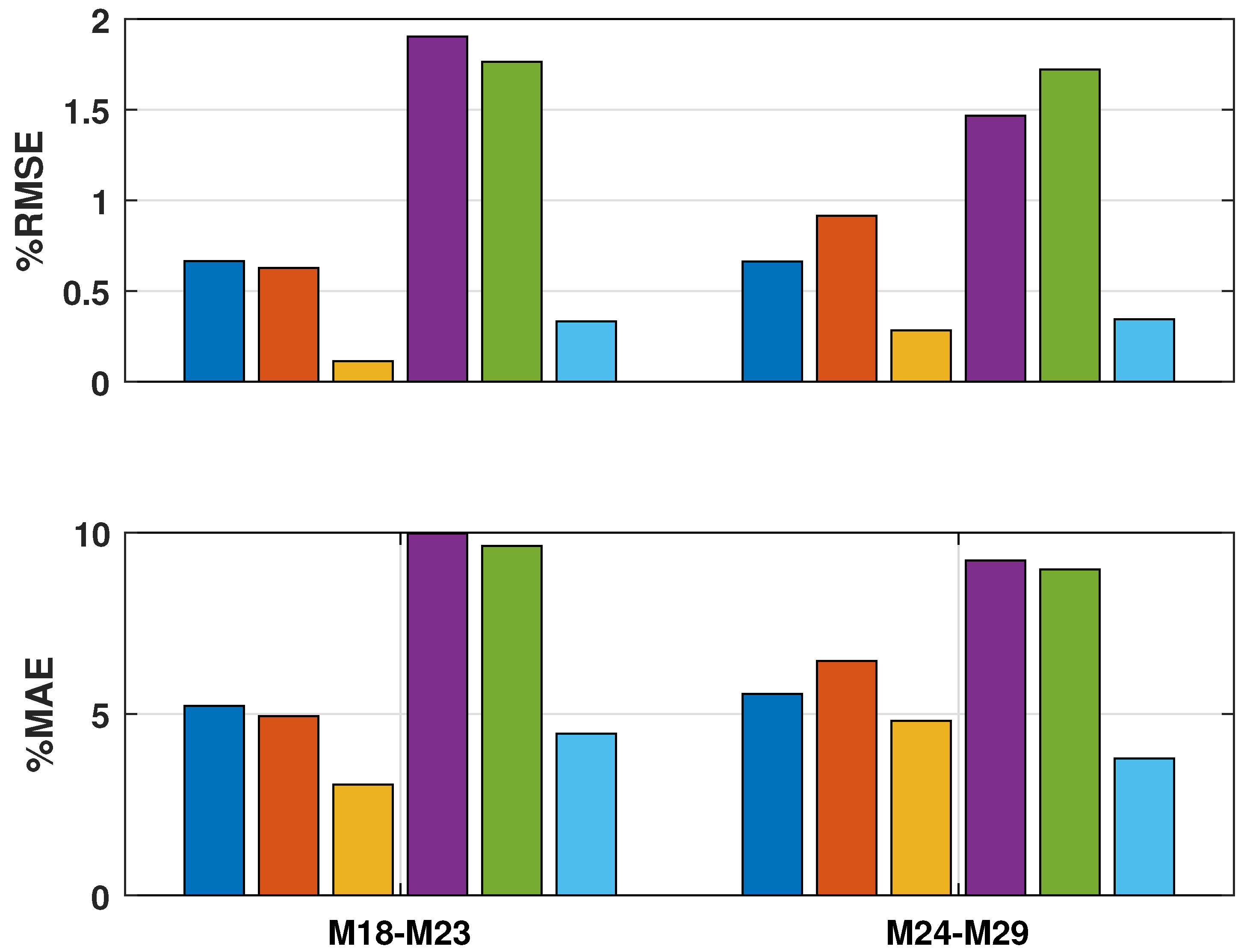
The important applications and framework of the MCNN are explained in Section 2.2 and Figure 4b. There are multiple works in the literature [48,49,59,60] in favor of multiple columns for image classification. Here, we tried to use the MCNN for regression on different inputs. The first is from satellite images at low spatial resolutions (1–4 km), but with more spatial coverage, roughly a 100 × 100 km2 grid area. Furthermore, the second is from ground spatial images at high resolutions with a low coverage area within 1 × 1 km 2 . The MCNN performed better for the multi-resolution input images, and the target was the in situ data. Actually, we performed the comparison at the ground level only. The comparison of the CNN-LSTM and MCNN for different data types such as GD, Sat, and the combined Sat-GD as the inputs were considered under the CR and CD conditions for time steps of 15 min, as shown in Figure 9. In Figure 9, [M18-M23] (left: 6-color bar) represents the CNN-LSTM model and [M24-M29] (right: 6-color bar) represents the MCNN model, whose details are given in Table 2. All these inputs were tested, and from the test response, we found that the ground-based approach showed a better response under both the CR and CD conditions due to the high-resolution spatial images. The multilevel stacking-based design of LSTM-MLP was used in the solar radiation forecasting, where a 6.08% RMSE was obtained in [32], whereas the CNN-LSTM [M18-M23] and MCNN [M24-M29] framework shown in Figure 9 achieved a <2% RMSE with Sat, GD, and Sat-GD as the inputs.

3.3. Effects of Cloudy Conditions

In Figure 10, the comparison of the hybrid forecasting model CNN-LSTM [M18,M19] and MCNN [M24,M25] under clear and cloudy sky conditions is shown separately. The top-left plot (Figure 10a) shows the actual and forecast power on a clear day using a dataset with 15 min time steps. The middle-left plot (Figure 10b) shows a linear regression graph of measured (actual) and predicted values on a clear day. The bottom-left plot (Figure 10c) shows the frequency of the forecast error graph of different models on a clear day. Similarly, all right-side plots represent a cloudy day. It is clearly shown in both conditions that the model prediction differed from clear day performance due to the non-linear nature of irradiance. Therefore, the linear regression and frequency distribution of the errors are scattered more in cloudy conditions in all three forecast plots.
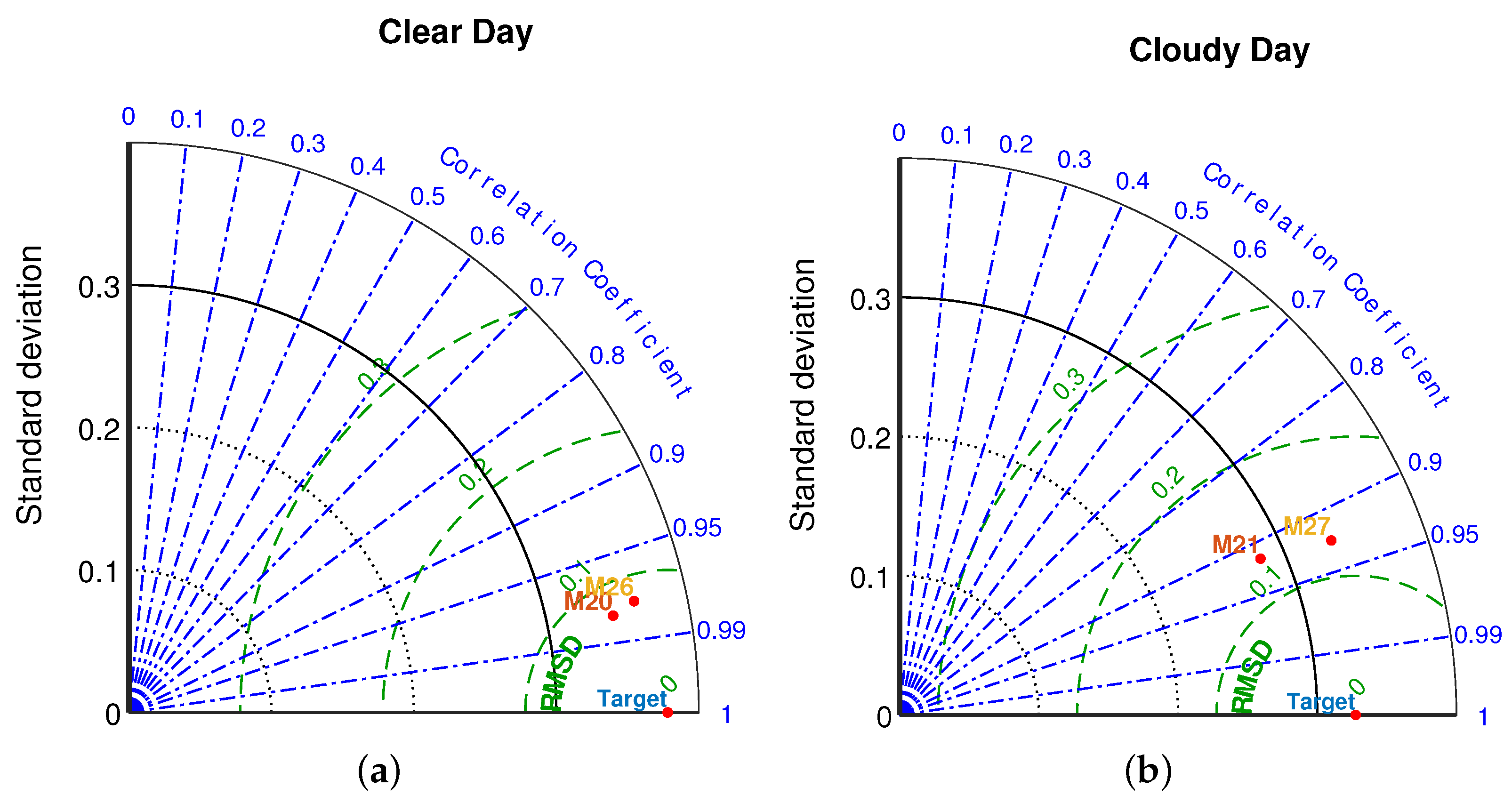
The Taylor diagram is an acceptable and suitable tool to reflect the comparison results and evaluation of different models in a graphical fashion. It provides a concise statistical summary of how well patterns match each other regarding their standard deviation, root-mean-squared deviations (RMSD), and the correlation coefficient. It was applied to compare different energy forecast frameworks such as [M18, M24] and [M19, M25] under a clear and cloudy day, respectively. For these Taylor diagrams, the lower-right corner (where the correlation coefficient I = 1 and RMSD = 0) was considered the ground truth or the measured values (observation point). Moving along the radial distance towards the origin indicates that the standard deviation decreases, while moving along the radial angle toward the bottom axis improves the correlation. With the enhancement in the standard deviation and correlation coefficient, the RMSD will decrease. The better model will be close to the observation point on the graph. As shown in Figure 11, for all forecast models, all correlation coefficients were in the range of [0.99–1.00] and [0.95–0.99] under clear and cloudy conditions, whereas the models’ RMSD lies in the range of [0–0.1]. The observation arc shows that the standard deviation of the models lies in the range of 0.3–0.4 for both conditions.

3.4. Effects of Satellite Inputs

We also compared the above methods with satellite datasets since satellite coverage has a greater spatial dimension with a low spatial and temporal resolution, but the cloud origin and movement are easily calculated in such a region. In the present simulation and forecasting models, the satellite coverage area was more than (10-times) the ground-based approach. As shown in Figure 12, for all forecast models [M20, M26] and [M21, M27], the correlation coefficients were in the range [0.95–0.99] under clear and [0.9–0.95] under cloudy days. In comparison, the RMSDs of the models were in the range of [0–0.1] for clear and [0.1–0.2] for cloudy days. The observation arc shows that all models’ standard deviations lie in the range of [0.3–0.4] for clear and [0.2–0.4] for cloudy days. The correlation coefficients, standard deviations, and RMSD parameters are desirable with the GD inputs compared to the Sat inputs because of the high spatial and temporal resolution, and hence, the GD-based approach is promising in comparison to the Sat-based on.

4. Conclusions

There are two basic problems when dealing with multiple data sources with the CNN. First, the application of the CNN to time series data is a bit difficult. Second, the handling of data with different spatial resolutions is challenging. For the first time, this paper assessed the potential of utilizing the convolutional neural network to forecast solar power using the multipoint and GCF approaches. The MCNN encodes the solar power from time series and spatial data to map the plants’ data into image matrices. The assessed results indicate that the ground-based approach with the multipoint input and output approach significantly improved the solar power generation forecast. In comparison with state-of-the-art time-series-based LSTM and image-based CNN, the multiple point approach offered 29.2060% and 36.5758% reductions in the MAE and 41.6292% and 56.4366% reductions in the RMSE. The spatial–temporal-based hybrid CNN-LSTM model outperformed all methods with the CR and CD conditions under the ground data.
Furthermore, the model was tested under the clear and cloudy conditions separately for the ground and satellite data to better analyze it. The findings for the proposed approach were best with the spatiotemporal ground inputs, as the correlation coefficients were in the range of [0.99–1.00] and [0.95–0.99] under clear and cloudy days, respectively, which are closer to the observational point, as shown in Figure 11. Furthermore, the CNN-LSTM and MCNN showed excellent performance with the ground-based spatiotemporal image in comparison with other approaches, with an RMSE of 0.3324% and 0.5826%, respectively, under cloudy conditions, for a 15 min-ahead forecast. The assessments of our approach could be further improved with more data points and more cloud information at multiple locations.

Author Contributions

Conceptualization, A.K.; methodology, A.K.; Supervision, Y.K. and P.K.; software, A.K.; Formal analysis, Y.K.; Investigation, Y.K and P.K.; data analysis, Y.K.; validation, A.K.; Visualization, Y.K.; writing—original draft, A.K.; Writing—review and editing, Y.K. and P.K. All authors have read and agreed to the published version of the manuscript.

Funding

This research received no external funding.

Data Availability Statement

Not applicable.

Acknowledgments

P.K. acknowledges the Eiffel project under grant agreement 101003518. The authors would also like to thank the National Institute of Technology Karnataka for providing the facilities to conduct this research work.

Conflicts of Interest

The authors declare no conflict of interest.

Nomenclature and Abbreviations

The following abbreviations are used in this manuscript:
M C C N Multi-column convolutional neural network
M T Multipoint time series
G C F Gramian cloud field matrix
P V Photovoltaic
C N N Convolutional neural network
L S T M Long short-term memory
D N N Deep neural network
F C Fully connected layer
R e g Regression
C P Cloud potential
M T y p e Model-type
D I Input dimension
T s Time series
S p Spatial
T p Temporal
S p T p Spatial–temporal
G D Ground
S a t Satellite
S a t G D Satellite–ground
C R Clear
C D Cloudy
C R C D Clear–cloudy
R M S E Root-mean-squared error
M A E Mean absolute error
R M S D        Root-mean-squared deviation
G H I Global horizontal irradiance
D N I Direct normal irradiance
D H I Diffuse horizontal irradiance
I N S Insolation

References

  1. Owusu, P.A.; Asumadu-Sarkodie, S. A review of renewable energy sources, sustainability issues and climate change mitigation. Cogent Eng. 2016, 3, 1167990. [Google Scholar] [CrossRef]
  2. Irfan, M.; Zhao, Z.Y.; Ahmad, M.; Mukeshimana, M.C. Solar energy development in Pakistan: Barriers and policy recommendations. Sustainability 2019, 11, 1206. [Google Scholar] [CrossRef] [Green Version]
  3. Das, L.; Habib, K.; Saidur, R.; Aslfattahi, N.; Yahya, S.M.; Rubbi, F. Improved thermophysical properties and energy efficiency of aqueous ionic liquid/mxene nanofluid in a hybrid pv/t solar system. Nanomaterials 2020, 10, 1372. [Google Scholar] [CrossRef]
  4. Chikh, M.; Berkane, S.; Mahrane, A.; Sellami, R.; Yassaa, N. Performance assessment of a 400 kWp multi-technology photovoltaic grid-connected pilot plant in arid region of Algeria. Renew. Energy 2021, 172, 488–501. [Google Scholar] [CrossRef]
  5. Yadav, H.K.; Pal, Y.; Tripathi, M.M. Photovoltaic power forecasting methods in smart power grid. In Proceedings of the 2015 Annual IEEE India Conference (INDICON), New Delhi, India, 17–20 December 2015; pp. 1–6. [Google Scholar]
  6. Ahmed, R.; Sreeram, V.; Mishra, Y.; Arif, M. A review and evaluation of the state-of-the-art in PV solar power forecasting: Techniques and optimization. Renew. Sustain. Energy Rev. 2020, 124, 109792. [Google Scholar] [CrossRef]
  7. Kumler, A.; Xie, Y.; Zhang, Y. A Physics-based Smart Persistence model for Intra-hour forecasting of solar radiation (PSPI) using GHI measurements and a cloud retrieval technique. Sol. Energy 2019, 177, 494–500. [Google Scholar] [CrossRef]
  8. Hajirahimi, Z.; Khashei, M. Hybrid structures in time series modeling and forecasting: A review. Eng. Appl. Artif. Intell. 2019, 86, 83–106. [Google Scholar] [CrossRef]
  9. Nayak, A.; Heistrene, L. Hybrid machine learning model for forecasting solar power generation. In Proceedings of the 2020 International Conference on Smart Grids and Energy Systems (SGES), Perth, Australia, 23–26 November 2020; pp. 910–915. [Google Scholar]
  10. de Freitas Viscondi, G.; Alves-Souza, S.N. A Systematic Literature Review on big data for solar photovoltaic electricity generation forecasting. Sustain. Energy Technol. Assess. 2019, 31, 54–63. [Google Scholar] [CrossRef]
  11. Sharifzadeh, M.; Sikinioti-Lock, A.; Shah, N. Machine-learning methods for integrated renewable power generation: A comparative study of artificial neural networks, support vector regression, and Gaussian Process Regression. Renew. Sustain. Energy Rev. 2019, 108, 513–538. [Google Scholar] [CrossRef]
  12. Marquez, R.; Pedro, H.T.; Coimbra, C.F. Hybrid solar forecasting method uses satellite imaging and ground telemetry as inputs to ANNs. Sol. Energy 2013, 92, 176–188. [Google Scholar] [CrossRef]
  13. Chu, Y.; Pedro, H.T.; Nonnenmacher, L.; Inman, R.H.; Liao, Z.; Coimbra, C.F. A smart image-based cloud detection system for intrahour solar irradiance forecasts. J. Atmos. Ocean. Technol. 2014, 31, 1995–2007. [Google Scholar] [CrossRef]
  14. Peng, Z.; Yu, D.; Huang, D.; Heiser, J.; Yoo, S.; Kalb, P. 3D cloud detection and tracking system for solar forecast using multiple sky imagers. Sol. Energy 2015, 118, 496–519. [Google Scholar] [CrossRef] [Green Version]
  15. Caldas, M.; Alonso-Suárez, R. Very short-term solar irradiance forecast using all-sky imaging and real-time irradiance measurements. Renew. Energy 2019, 143, 1643–1658. [Google Scholar] [CrossRef]
  16. Joshi, J.C.; Kaur, P.; Kumar, B.; Singh, A.; Satyawali, P. HIM-STRAT: A neural network-based model for snow cover simulation and avalanche hazard prediction over North-West Himalaya. Nat. Hazards 2020, 103, 1239–1260. [Google Scholar] [CrossRef]
  17. Zamora, R.J.; Dutton, E.G.; Trainer, M.; McKeen, S.A.; Wilczak, J.M.; Hou, Y.T. The accuracy of solar irradiance calculations used in mesoscale numerical weather prediction. Mon. Weather Rev. 2005, 133, 783–792. [Google Scholar] [CrossRef]
  18. Lima, F.J.; Martins, F.R.; Pereira, E.B.; Lorenz, E.; Heinemann, D. Forecast for surface solar irradiance at the Brazilian Northeastern region using NWP model and artificial neural networks. Renew. Energy 2016, 87, 807–818. [Google Scholar] [CrossRef]
  19. Ji, W.; Chee, K.C. Prediction of hourly solar radiation using a novel hybrid model of ARMA and TDNN. Sol. Energy 2011, 85, 808–817. [Google Scholar] [CrossRef]
  20. Bhardwaj, S.; Sharma, V.; Srivastava, S.; Sastry, O.; Bandyopadhyay, B.; Chandel, S.; Gupta, J. Estimation of solar radiation using a combination of Hidden Markov Model and generalized Fuzzy model. Sol. Energy 2013, 93, 43–54. [Google Scholar] [CrossRef]
  21. Voyant, C.; Muselli, M.; Paoli, C.; Nivet, M.L. Hybrid methodology for hourly global radiation forecasting in Mediterranean area. Renew. Energy 2013, 53, 1–11. [Google Scholar] [CrossRef] [Green Version]
  22. Dong, Z.; Yang, D.; Reindl, T.; Walsh, W.M. Short-term solar irradiance forecasting using exponential smoothing state space model. Energy 2013, 55, 1104–1113. [Google Scholar] [CrossRef]
  23. Hajihassani, M.; Jahed Armaghani, D.; Kalatehjari, R. Applications of particle swarm optimization in geotechnical engineering: A comprehensive review. Geotech. Geol. Eng. 2018, 36, 705–722. [Google Scholar] [CrossRef]
  24. Baser, F.; Demirhan, H. A fuzzy regression with support vector machine approach to the estimation of horizontal global solar radiation. Energy 2017, 123, 229–240. [Google Scholar] [CrossRef]
  25. Mohammadi, K.; Shamshirband, S.; Tong, C.W.; Arif, M.; Petković, D.; Ch, S. A new hybrid support vector machine–wavelet transform approach for estimation of horizontal global solar radiation. Energy Convers. Manag. 2015, 92, 162–171. [Google Scholar] [CrossRef]
  26. Deo, R.C.; Wen, X.; Qi, F. A wavelet-coupled support vector machine model for forecasting global incident solar radiation using limited meteorological dataset. Appl. Energy 2016, 168, 568–593. [Google Scholar] [CrossRef]
  27. Hussain, S.; Al Alili, A. A pruning approach to optimize synaptic connections and select relevant input parameters for neural network modelling of solar radiation. Appl. Soft Comput. 2017, 52, 898–908. [Google Scholar] [CrossRef]
  28. Lan, H.; Yin, H.; Hong, Y.Y.; Wen, S.; David, C.Y.; Cheng, P. Day-ahead spatio-temporal forecasting of solar irradiation along a navigation route. Appl. Energy 2018, 211, 15–27. [Google Scholar] [CrossRef]
  29. Davò, F.; Alessandrini, S.; Sperati, S.; Delle Monache, L.; Airoldi, D.; Vespucci, M.T. Post-processing techniques and principal component analysis for regional wind power and solar irradiance forecasting. Sol. Energy 2016, 134, 327–338. [Google Scholar] [CrossRef] [Green Version]
  30. Li, P.; Zhou, K.; Lu, X.; Yang, S. A hybrid deep learning model for short-term PV power forecasting. Appl. Energy 2020, 259, 114216. [Google Scholar] [CrossRef]
  31. de Jesús, D.A.R.; Mandal, P.; Chakraborty, S.; Senjyu, T. Solar PV Power Prediction Using A New Approach Based on Hybrid Deep Neural Network. In Proceedings of the 2019 IEEE Power & Energy Society General Meeting (PESGM), Atlanta, GA, USA, 4–8 August 2019; pp. 1–5. [Google Scholar] [CrossRef]
  32. Al-Hajj, R.; Assi, A.; Fouad, M.M. Multi-level Stacking of Long Short Term Memory Recurrent Models for Time Series Forecasting of Solar Radiation. In Proceedings of the 2021 10th International Conference on Renewable Energy Research and Application (ICRERA), Ankara, Turkey, 26–29 September 2021; pp. 71–76. [Google Scholar]
  33. Munkhammar, J.; Widén, J.; Hinkelman, L.M. A copula method for simulating correlated instantaneous solar irradiance in spatial networks. Sol. Energy 2017, 143, 10–21. [Google Scholar] [CrossRef]
  34. Yuan, Z.; Zhou, X.; Yang, T. Hetero-convlstm: A deep learning approach to traffic accident prediction on heterogeneous spatio-temporal data. In Proceedings of the Proceedings of the 24th ACM SIGKDD International Conference on Knowledge Discovery & Data Mining, London, UK, 19–23 August 2018; pp. 984–992. [Google Scholar]
  35. Drineas, P.; Mahoney, M.W. Approximating a gram matrix for improved kernel-based learning. In Proceedings of the International Conference on Computational Learning Theory, Paris, France, 3–6 July 2005; Springer: Berlin/Heidelberg, Germany, 2005; pp. 323–337. [Google Scholar]
  36. Xiong, J.; Li, C.; Wang, C.D.; Cen, J.; Wang, Q.; Wang, S. Application of Convolutional Neural Network and Data Preprocessing by Mutual Dimensionless and Similar Gram Matrix in Fault Diagnosis. IEEE Trans. Ind. Inform. 2022, 18, 1061–1071. [Google Scholar] [CrossRef]
  37. Lim, S.C.; Huh, J.H.; Hong, S.H.; Park, C.Y.; Kim, J.C. Solar Power Forecasting Using CNN-LSTM Hybrid Model. Energies 2022, 15, 8233. [Google Scholar] [CrossRef]
  38. Mayer, B.; Kylling, A. The libRadtran software package for radiative transfer calculations-description and examples of use. Atmos. Chem. Phys. 2005, 5, 1855–1877. [Google Scholar] [CrossRef] [Green Version]
  39. Emde, C.; Buras-Schnell, R.; Kylling, A.; Mayer, B.; Gasteiger, J.; Hamann, U.; Kylling, J.; Richter, B.; Pause, C.; Dowling, T.; et al. The libRadtran software package for radiative transfer calculations (version 2.0. 1). Geosci. Model Dev. 2016, 9, 1647–1672. [Google Scholar] [CrossRef] [Green Version]
  40. Kosmopoulos, P.G.; Kazadzis, S.; Taylor, M.; Raptis, P.I.; Keramitsoglou, I.; Kiranoudis, C.; Bais, A.F. Assessment of surface solar irradiance derived from real-time modelling techniques and verification with ground-based measurements. Atmos. Meas. Tech. 2018, 11, 907–924. [Google Scholar] [CrossRef] [Green Version]
  41. Masoom, A.; Kosmopoulos, P.; Bansal, A.; Kazadzis, S. Solar energy estimations in India using remote sensing technologies and validation with sun photometers in urban areas. Remote Sens. 2020, 12, 254. [Google Scholar] [CrossRef] [Green Version]
  42. Ricchiazzi, P.; Yang, S.; Gautier, C.; Sowle, D. SBDART: A research and teaching software tool for plane-parallel radiative transfer in the Earth’s atmosphere. Bull. Am. Meteorol. Soc. 1998, 79, 2101–2114. [Google Scholar] [CrossRef]
  43. Kato, S.; Ackerman, T.P.; Mather, J.H.; Clothiaux, E.E. The k-distribution method and correlated-k approximation for a shortwave radiative transfer model. J. Quant. Spectrosc. Radiat. Transf. 1999, 62, 109–121. [Google Scholar] [CrossRef]
  44. Shettle, E. Models of aerosols, clouds and precipitation for atmospheric propagation studies, paper presented at Conference on Atmospheric Propagation in the UV, Visible, IR and MM-Region and Related System Aspects, NATO Adv. Group for Aerosp. Res. Dev. Cph. 1989. [Google Scholar]
  45. Albawi, S.; Mohammed, T.A.; Al-Zawi, S. Understanding of a convolutional neural network. In Proceedings of the 2017 International Conference on Engineering and Technology (ICET), Antalya, Turkey, 21–23 August 2017; pp. 1–6. [Google Scholar]
  46. Sherstinsky, A. Fundamentals of recurrent neural network (RNN) and long short-term memory (LSTM) network. Phys. D Nonlinear Phenom. 2020, 404, 132306. [Google Scholar] [CrossRef] [Green Version]
  47. Sainath, T.N.; Vinyals, O.; Senior, A.; Sak, H. Convolutional, long short-term memory, fully connected deep neural networks. In Proceedings of the 2015 IEEE International Conference on Acoustics, Speech and Signal Processing (ICASSP), Queensland, Australia, 19–24 April 2015; pp. 4580–4584. [Google Scholar]
  48. Yang, H.; Han, J.; Min, K. A multi-column CNN model for emotion recognition from EEG signals. Sensors 2019, 19, 4736. [Google Scholar] [CrossRef]
  49. Ouyang, X.; Xu, S.; Zhang, C.; Zhou, P.; Yang, Y.; Liu, G.; Li, X. A 3D-CNN and LSTM based multi-task learning architecture for action recognition. IEEE Access 2019, 7, 40757–40770. [Google Scholar] [CrossRef]
  50. Olmschenk, G.; Tang, H.; Zhu, Z. Improving dense crowd counting convolutional neural networks using inverse k-nearest neighbor maps and multiscale upsampling. arXiv 2019, arXiv:1902.05379. [Google Scholar]
  51. Xiao, M.; Wu, Y.; Zuo, G.; Fan, S.; Yu, H.; Shaikh, Z.A.; Wen, Z. Addressing Overfitting Problem in Deep Learning-Based Solutions for Next Generation Data-Driven Networks. Wirel. Commun. Mob. Comput. 2021, 2021. [Google Scholar] [CrossRef]
  52. Javid, A.M.; Das, S.; Skoglund, M.; Chatterjee, S. A ReLU Dense Layer to Improve the Performance of Neural Networks. In Proceedings of the ICASSP 2021—2021 IEEE International Conference on Acoustics, Speech and Signal Processing (ICASSP), Toronto, ON, Canada, 6–11 June 2021; pp. 2810–2814. [Google Scholar] [CrossRef]
  53. Xie, J.; Chen, B.; Gu, X.; Liang, F.; Xu, X. Self-attention-based BiLSTM model for short text fine-grained sentiment classification. IEEE Access 2019, 7, 180558–180570. [Google Scholar] [CrossRef]
  54. Aslan, M.F.; Unlersen, M.F.; Sabanci, K.; Durdu, A. CNN-based transfer learning–BiLSTM network: A novel approach for COVID-19 infection detection. Appl. Soft Comput. 2021, 98, 106912. [Google Scholar] [CrossRef]
  55. Yongsheng, D.; Fengshun, J.; Jie, Z.; Zhikeng, L. A short-term power output forecasting model based on correlation analysis and ELM-LSTM for distributed PV system. J. Electr. Comput. Eng. 2020, 2020. [Google Scholar] [CrossRef]
  56. Qu, J.; Qian, Z.; Pei, Y. Day-ahead hourly photovoltaic power forecasting using attention-based CNN-LSTM neural network embedded with multiple relevant and target variables prediction pattern. Energy 2021, 232, 120996. [Google Scholar] [CrossRef]
  57. Tovar, M.; Robles, M.; Rashid, F. PV power prediction, using CNN-LSTM hybrid neural network model. Case of study: Temixco-Morelos, México. Energies 2020, 13, 6512. [Google Scholar] [CrossRef]
  58. Zang, H.; Cheng, L.; Ding, T.; Cheung, K.W.; Liang, Z.; Wei, Z.; Sun, G. Hybrid method for short-term photovoltaic power forecasting based on deep convolutional neural network. IET Gener. Transm. Distrib. 2018, 12, 4557–4567. [Google Scholar] [CrossRef]
  59. Yan, R.; Liao, J.; Yang, J.; Sun, W.; Nong, M.; Li, F. Multi-hour and multi-site air quality index forecasting in Beijing using CNN, LSTM, CNN-LSTM, and spatiotemporal clustering. Expert Syst. Appl. 2021, 169, 114513. [Google Scholar] [CrossRef]
  60. Gao, B.; Huang, X.; Shi, J.; Tai, Y.; Zhang, J. Hourly forecasting of solar irradiance based on CEEMDAN and multi-strategy CNN-LSTM neural networks. Renew. Energy 2020, 162, 1665–1683. [Google Scholar] [CrossRef]
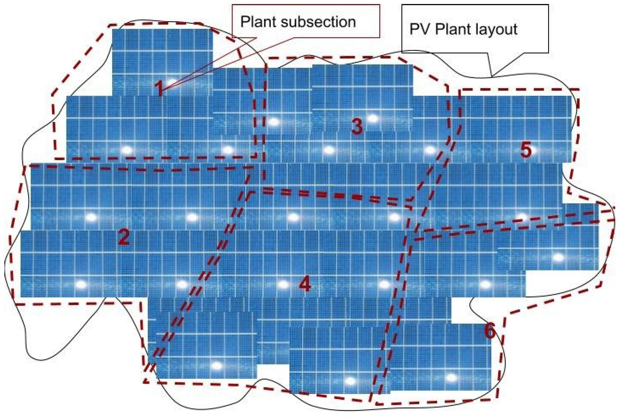
Figure 1. The spatial distribution of PV plants’ layout and data collection regions.
Remotesensing 15 00107 g001
Figure 2. Time series-to-spatial–temporal image matrix conversion: (a) variation of power over space (red color) and time (black color); (b) time domain image matrix derived from Equation (1); (c) spacial domain image matrix derived from Equation (1); (d) time domain GCF image; (e) space domain GCF image; (f) time–space domain GCF image.
Remotesensing 15 00107 g002
Figure 3. The satellite irradiance components DHI, DNI, GHI, and insolation (INS).
Remotesensing 15 00107 g003
Figure 4. The DNN model networks’ structure with GD, Sat, and Sat-GD data as the input: (a) The framework of the CNN-LSTM model. (b) The framework of the MCNN model.
Remotesensing 15 00107 g004
Figure 5. Comparison of the single- versus multiple-point approach: (a) single vs. multiple inputs; (b) single vs. multiple inputs; (c) single vs. multiple outputs; (d) single vs. multiple outputs.
Remotesensing 15 00107 g005
Figure 6. Comparison of spatial, temporal, spatial–temporal, and mixed approaches: (a) spatial input; (b) spatial output; (c) temporal input; (d) temporal output; (e) spatial–temporal input; (f) spatial–temporal output; (g) mixed approaches; (h) mixed approaches.
Remotesensing 15 00107 g006
Figure 7. Comparison of the 22 locations of solar plants at 90 min time steps.
Remotesensing 15 00107 g007
Figure 8. The absolute errors of the 22 locations at 15 min-timesteps.
Remotesensing 15 00107 g008
Figure 9. Comparison of different models under clear and cloudy days with GD, Sat, and Sat-GD inputs, when time steps = 15.
Remotesensing 15 00107 g009
Figure 10. Comparison of different models under clear and cloudy days at time steps = 15: (a) Power prediction under clear sky. (b) Power prediction under cloudy sky. (c) Scatter plot under clear sky. (d) Scatter plot under cloudy sky. (e) Frequency of forecast error under clear sky. (f) Frequency of forecast error under cloudy sky.
Remotesensing 15 00107 g010
Figure 11. Comparison of clear and cloudy days when time steps = 15: (a) Clear sky. (b) Cloudy sky.
Remotesensing 15 00107 g011
Figure 12. Comparison of clear and cloudy days for satellite data when time steps = 15: (a) Clear sky. (b) Cloudy sky.
Remotesensing 15 00107 g012
Table 1. Model properties.
SettingsParameters
Solar dataset number22
Training set size72,576
LSTM network layer number6
LSTM neuron number in each layer100
CNN network layer number6
CNN neuron number in each layer100
LSTM-CNN network layer number12
LSTM-CNN neuron number in each layer100
Hidden dense layer number2
Hidden neuron number200, 200
Dropout rate0.2
Training methodAdam optimizer
Loss functionRMSE, MAE
Forecast horizon (min)5–120 (2-h)
Table 3. Metrics of methods with time steps.
ModelMAERMSE
153090153090
M127.220327.540524.72399.759010.32848.4229
M29.577015.322425.22581.54533.15439.0886
M317.394012.396420.93504.78242.25676.2924
M426.241726.259526.34329.07469.09609.1694
M525.869625.886625.97078.82278.83788.9141
M626.241926.259826.34539.07779.09829.1745
M78.470410.705419.96111.46912.12975.4158
M825.967424.860526.33038.86898.08519.1643
M913.793412.020820.10832.83522.27005.4955
M1020.675714.486620.88886.48443.15015.9975
M1113.904115.996122.41803.17083.81446.8712
M128.957512.147520.96641.58732.45015.9187
M139.079411.993320.90831.56722.33155.9165
M149.238010.448815.78621.67602.07374.1134
M158.987210.659215.31561.55111.99173.6687
M168.991110.974915.35691.65732.28853.9627
M178.797110.677314.87661.59222.12813.5232
M183.05802.17125.03910.11350.10930.7463
M194.45614.48779.99520.33240.37961.2174
M204.93875.142810.99530.62600.80582.6585
M219.63069.935413.28871.76361.84703.3160
M225.21875.472711.46580.66400.86642.7936
M239.974010.645715.45601.90312.58894.8156
M244.81583.55405.50370.28260.28260.4237
M255.02464.53489.31280.58260.57521.7748
M265.84348.0384419.67180.73571.88138.7471
M278.98038.939819.06661.72131.76626.0082
M285.55347.094018.92870.66131.15345.9412
M299.22679.517918.31951.46691.89965.8551
Disclaimer/Publisher’s Note: The statements, opinions and data contained in all publications are solely those of the individual author(s) and contributor(s) and not of MDPI and/or the editor(s). MDPI and/or the editor(s) disclaim responsibility for any injury to people or property resulting from any ideas, methods, instructions or products referred to in the content.