Abstract
Vegetation isoline equations describe analytical relationships between two reflectances of different wavelengths. Their applications range from retrievals of biophysical parameters to the derivation of the inter-sensor relationships of spectral vegetation indexes. Among the three variants of vegetation isoline equations introduced thus far, the optimized asymmetric-order vegetation isoline equation is the newest and is known to be the most accurate. This accuracy assessment, however, has been performed only for the wavelength pair of red and near-infrared (NIR) bands fixed at ∼655 nm and ∼865 nm, respectively. The objective of this study is to extend this wavelength limitation. An accuracy assessment was therefore performed over a wider range of wavelengths, from 400 to 1200 nm. The optimized asymmetric-order vegetation isoline equation was confirmed to demonstrate the highest accuracy among the three isolines for all the investigated wavelength pairs. The second-best equation, the asymmetric-order isoline equation, which does not include an optimization factor, was not superior to the least-accurate equation (i.e., the first-order isoline equation) in some cases. This tendency was prominent when the reflectances of the two wavelengths were similar. By contrast, the optimized asymmetric-order vegetation isoline showed stable performance throughout this study. A single factor introduced into the optimized asymmetric-order isoline equation was concluded to effectively reduce errors in the isoline for all the wavelength combinations examined in this study.
Keywords:
vegetation isoline; higher-order interaction; asymmetric; VI; LAI; RT model; inversion; hyperspectral data 1. Introduction
Remotely sensed reflectance spectra have been used to estimate biophysical parameters for terrestrial vegetation [1,2]. The simplest and most widely accepted approach for this purpose is to use a spectral vegetation index (VI). Because VIs are often defined as algebraic manipulations of reflectance spectra, VI model equations are also considered a relationship that the reflectance spectrum should satisfy under a fixed biophysical parameter. In particular, a fundamental relationship between the reflectances of two bands (e.g., red and near-infrared (NIR) bands) has been the basis of numerous VIs [3,4,5,6,7,8,9]. This relationship is known as a vegetation isoline equation. The vegetation isoline concept has been investigated intensively over the past two decades [10,11,12,13,14,15] and is considered a useful tool [11,16,17] to explore various applications [18,19].
The concept of vegetation isolines originated from investigations examining the influence of soil brightness on VIs [3,20]. In general, soil brightness varies considerably with changes in soil moisture, surface roughness, shadow amount, and soil characteristics such as organic matter content [21,22,23,24]. These variations affect the soil background component of reflectance spectra, which leads to variations in VI values [16,17]. This effect, known as soil noise, has been a major issue in the field of land remote sensing. Studies seeking to minimize soil noise have paid particular attention analytically to a spectral trajectory observed in the red–NIR reflectance subspace under a constant canopy [3,7]. The derived concept, the vegetation isoline, has been applied to solve the issue of the influence of soil brightness, which has affected various VIs to some extent [3,4,5,6,9,25].
The applications of the vegetation isoline concept are not limited to the analyses of VIs. It can also be used to directly retrieve biophysical parameters such as the fraction of vegetation cover (FVC), leaf area index (LAI), and the chlorophyll-a and -b contents [19,26,27,28]. In addition, vegetation isoline equations that represent an analytical relationship of two reflectances have been used in investigations of inter-sensor VI translation [18,29,30,31,32,33] in the context of satellite constellations. The derivations of such isoline equations require several simplifications of the model, which somewhat restricts their range of applications.
A system of vegetation canopy that is assumed for deriving vegetation isoline equations consists of a canopy layer, which is considered a turbid medium, and a soil layer of a Lambertian surface underneath the canopy. For this system of layers, a top-of-the-canopy (TOC) reflectance is represented by an analytical model known as the successive order of scattering, in which the TOC reflectance is modeled by the sum of all the photons categorized by the number of interactions between the soil surface and the canopy layers. For example, the photons scattered only once by the soil surface are labeled as the first-order interaction term. Using this analytical representation of TOC reflectance, the initial attempt to derive a vegetation isoline equation was conducted by truncating the second-order and the higher-order interaction terms between the vegetation canopy and soil surfaces [3,10]. The obtained isoline equation is referred to as the first-order vegetation isoline because the isoline equation accounts only for the first-order interaction term. Although the derived isoline equation is simple and suitable for the analyses of VIs, the simplification associated with the truncation adversely affects its accuracy, especially when the soil brightness is high. Researchers would later develop methods to overcome this weakness.
In our previous work, we improved the accuracy of the first-order vegetation isoline by accounting for the higher-order interaction term during the derivation. This improvement was performed for the widely used red and NIR wavelengths. The derived form is referred to as the asymmetric-order vegetation isoline equation because the second-order interaction term is retained only in the NIR wavelength [13]. In addition, the accuracy of the asymmetric-order vegetation isoline equation was improved dramatically by the introduction of a single factor. The derived new isoline equation was named the “optimized” asymmetric-order vegetation isoline equation [14,15]. Errors in the optimized asymmetric-order isoline equation were reduced to 4% relative to the errors in the first-order isoline equation [13] and were also reduced to 20% relative to the errors in the asymmetric-order isoline equation [14]. After this improvement, the errors in the optimized asymmetric-order isoline equations were smaller in magnitude than the magnitude equivalent to the signal-to-noise ratio (SNR) of some existing sensors.
The accuracy improvements and evaluations of the vegetation isoline equations reported in the previous works were limited to the pair of red and NIR bands—specifically, those at ∼655 nm and ∼865 nm, respectively. This limitation should be extended to make the derived isoline equations more useful for a broader range of applications. One such application is hyperspectral sensors. In recent years, numerous hyperspectral sensors have been available for Earth observation, and new missions are underway [34,35,36,37,38,39,40]. Such hyperspectral sensors enable us to process more than one hundred bands, which could improve the accuracy in biophysical parameter retrievals. For these motivations, the wavelength range should be extended to a broader range of visible-to-NIR wavelengths.
In the present work, the accuracies of the three variants of the vegetation isoline equations are evaluated in the wavelength range from 400 to 1200 nm on the basis of numerical simulations by a radiative transfer model. The explanation that follows starts with the introduction of the three variants of the vegetation isoline equations. The numerical experiments and their results are then described to evaluate their accuracy in a wide range of wavelengths. Finally, the results are further discussed and the study is concluded with descriptions of some unresolved issues.
2. Three Variants of Vegetation Isoline Equations
2.1. First-Order Vegetation Isoline Equation
The first derivation of a vegetation isoline equation began with the approximation of a linear relationship between reflectances measured at two distinct wavelengths, and . During the derivation, the well-known concept of the soil line [41] was assumed. The derived relationship is known as the first-order approximated vegetation isoline equation. During the derivation of the first-order vegetation isoline, the second- and higher-order interaction terms were truncated. The isoline equation is expressed by
with and defined as
where is the FVC defined as a vertically projected area of vegetation canopy [42], and are the TOC reflectances of the different wavelengths, and are the “pure” canopy reflectances (canopy path radiance), which are independent of the soil surface beneath the canopy layer, and and represent the two-way transmittances of the vegetation canopy, , averaged over a target area with the FVC, , as its weight. The contribution of higher-order interaction terms is represented by . The two constants, a and b, are the soil line slope and offset, respectively. Although the derived expression is simple and sufficiently accurate to analyze the performance of VIs, the truncation error represented by tends to be large when the soil reflectance becomes high [10,11]. In recent years, this shortcoming has been overcome through a unique approach described in the next subsection.
2.2. Asymmetric-Order Vegetation Isoline Equation
The asymmetric-order form was derived by including the interaction terms up to the second-order in ; by contrast, in , only the terms up to the first-order interaction were considered [13]. The derived asymmetric-order vegetation isoline equation becomes
with the following definitions:
where represents the bi-hemispherical reflectance of the canopy layer at the bottom surface, which appears only in the band . The contribution of higher-order interaction terms in this case is represented by , which is considered a truncation error during numerical simulation.
The error of the derived isoline equation is decreased dramatically from that of the first-order form [14]. Most notably, this increase in accuracy was achieved without losing its simplicity in the analytical expression. To improve the accuracy one step further, a single factor was introduced into the derived expression, which is considered the “optimized” asymmetric-order vegetation isoline equation.
2.3. Optimized Asymmetric-Order Vegetation Isoline Equation
The optimized asymmetric-order vegetation isoline equation was obtained by introducing a single factor k into the asymmetric-order form of the equation. After neglecting the higher-order interaction term in Equation (5) [14], the factor k is introduced in the third term of the right-hand side,
The newly introduced factor k can be derived by solving Equation (11) for k:
This representation of k implies that the factor depends on biophysical parameters, as well as soil line parameters. That is, the factor is not a constant in this context. At the same time, if we replace k by a constant, there would be an optimum value. Even though the actual k is not a constant, such an “optimum” value for k can be expected to minimize the error to some extent. Again, k in Equation (12) depends on the biophysical and soil line parameters. It is not realistic, however, to find both biophysical- and soil-dependent k in actual satellite data. To solve this problem, we attempted to find a constant factor as k for each “wavelength pair” that minimizes the error of the isoline equation on the basis of numerical simulations. In summary, the optimum constant factor for the replacement of the variable k would depend heavily on the choice of the wavelength pairs ( and ), which is the central theme of the present study.
2.4. Demonstration of the Errors in the Vegetation Isoline Equations
In this subsection, we demonstrate the accuracy improvement of the isoline equations by comparing the three forms of the previously introduced isolines. The errors of the three isoline equations were simulated numerically by a radiative transfer (RT) model. In this demonstration, the wavelength pair and was fixed at 655 nm (red) and 865 nm (NIR), respectively. The PROSAIL model [43] was used to simulate both the spectral reflectance as a function of the LAI and the soil reflectance spectra (from dark to bright soil). The parameter settings of the RT model and the retrieval algorithms of the isoline parameters [13,14] will be further explained in the following section.
Figure 1 shows the errors in the three forms of isolines (the top, middle, and bottom plots correspond to the first-order, asymmetric-order, and optimized asymmetric-order forms, respectively) as a function of the LAI and soil reflectance of the red wavelength represented by . The left and right columns in Figure 1 correspond to the cases of FVC = 1.0 and 0.5, respectively. The error observed in the asymmetric-order form is smaller than that in the first-order form, but it increases with increasing soil brightness. On the contrary, the errors in the optimized asymmetric-order form are much smaller than those in the other two forms even in cases where the soil brightness increased. This accuracy improvement is a result of our optimization of the single factor introduced into the asymmetric-order vegetation isoline equation [14].
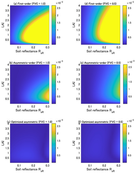
Figure 1.
Errors in the first-order isoline equation (upper panels, (a,d)), asymmetric-order isoline equation (middle panels, (b,e)), and optimized asymmetric-order isoline equation (bottom panels, (c,f)) for red and NIR wavelength pairs as a function of the LAI and soil reflectance. The FVC is 1.0 for the left panels (a–c) and 0.5 for the right panels (d–f).
3. Numerical Simulations of Vegetation Isolines
3.1. Parameter Settings of Simulations to Determine Vegetation Isolines
Numerical simulations of vegetation isoline equations (Equations (1), (5), and (11)) were conducted with various settings of the LAI, FVC, and soil brightness for a wide range of wavelength (band) pairs. TOC reflectance spectra were computed using a well-known canopy radiative transfer code, PROSAIL [43], which is a combination of the leaf optical properties model PROSPECT [44] and the canopy bidirectional reflectance model SAIL [45]. The parameter settings in the simulations are summarized in Table 1. The LAI was varied from 0.0 to 4.0 in increments of 0.8 (six variants). The soil brightness is represented by the factor “psoil” in the model, which was varied from 0.0 to 1.0 in increments of 0.2 (six variants). The factor psoil represents the mixture ratio of the two representative soil spectra (i.e., a wet soil spectrum and a dry soil spectrum) implemented in the RT model. The canopy reflectance spectra obtained using PROSAIL were linearly mixed with the soil spectra using the FVC, , as the weight, which was varied from 0.0 to 1.0 in increments of 0.2 (six variants).

Table 1.
Input parameters used in the numerical simulations [14].
For the leaf angle distribution (LAD), the spherical distribution model was assumed. The other input parameters for PROSAIL were also fixed throughout the study, as summarized in Table 1. Note that a single mesophyll size was assumed throughout the simulation. Furthermore, note that the hotspot size parameter was assumed to be 0.01 to avoid the strong contribution of this effect during the simulation. The total number of parameter combinations was therefore 216 (6 × 6 × 6). The isoline equations for these conditions were simulated for each pair of wavelengths, and , where was varied from 410 to 1200 nm in 10 nm intervals (total of 80 discrete bands) and was varied from 400 to minus 10 nm at 10 nm intervals, resulting in a total of (=3160) combinations. In summary, for each pair of wavelength (band) combinations (3160 pairs), a total of 216 TOC reflectance spectra were obtained by the numerical simulations.
The algorithm used to determine the parameters in the vegetation isoline equations is identical to that used in numerous previous studies [10,11,12,13,14]. The canopy reflectance parameter was computed using the spectrally flat zero reflectance of the soil surface. The two-way transmittances for vegetation canopy, , were approximated on the basis of the simulated TOC reflectance with a soil reflectance of medium brightness, where was computed in the previous step [14]. In the simulation, the TOC reflectances in the were approximated from the first- and the second-order interaction terms between the canopy layer and the soil surface:
where represents the bi-hemispherical reflectance of the soil surface for the band. The spherical albedo of the canopy layer, , was obtained by solving Equation (13) for , in which the soil spectrum was brighter than that in the simulation used to compute . The soil spectrum was also spectrally flat in this case [13]. The slope and offset of the soil line equation over the and reflectance space were obtained by linear regression of the reflectance spectra for the wet and dry soils (Table 1). The TOC reflectance spectra used to depict true isolines were simply the output of PROSAIL under the assumption of zero-brightness soil.
3.2. Definition of Errors in Isoline Equations and Determination of the Optimum Value of
Errors of the vegetation isoline equations were measured using the distance between the true and the approximated isolines ():
where represents the spectrum derived by asymmetric-order vegetation isoline equations as a function of k and denotes the spectrum on the vegetation isoline including all the higher-order interaction terms (i.e., the true spectrum). Note that the first-order and the asymmetric-order isoline equations correspond to the cases of and in Equation (11); thus, the errors in the three isoline equations can be simply measured using Equation (14). We again note that the RT simulations were conducted with 216 different parameter settings, which resulted in 216 different values of for each pair of and . For the sake of total evaluation, these values were averaged over the 216 simulation cases to obtain a mean error represented by . In the following discussion, we use the term “mean error” and “mean epsilon, ”, interchangeably because, as previously described, Equation (14) (i.e., ) can be applicable to all the cases when k is set appropriately.
The optimum value of k in Equation (11) for each wavelength pair was explored on the basis of . First, the values of k were computed from Equation (12) for all 216 parameter combinations. The maximum and minimum were then found among the 216 different k values. Finally, within the range of the maximum and minimum values, the optimum value of k, referred to as , was searched, which resulted in a minimum of the mean (i.e., the minimum of ) [14,15]. Apparently, this minimum of is identical to the mean of (i.e., ), which is defined as the mean error (or mean epsilon) of the optimized asymmetric-order vegetation isoline.
4. Results
4.1. Analysis of
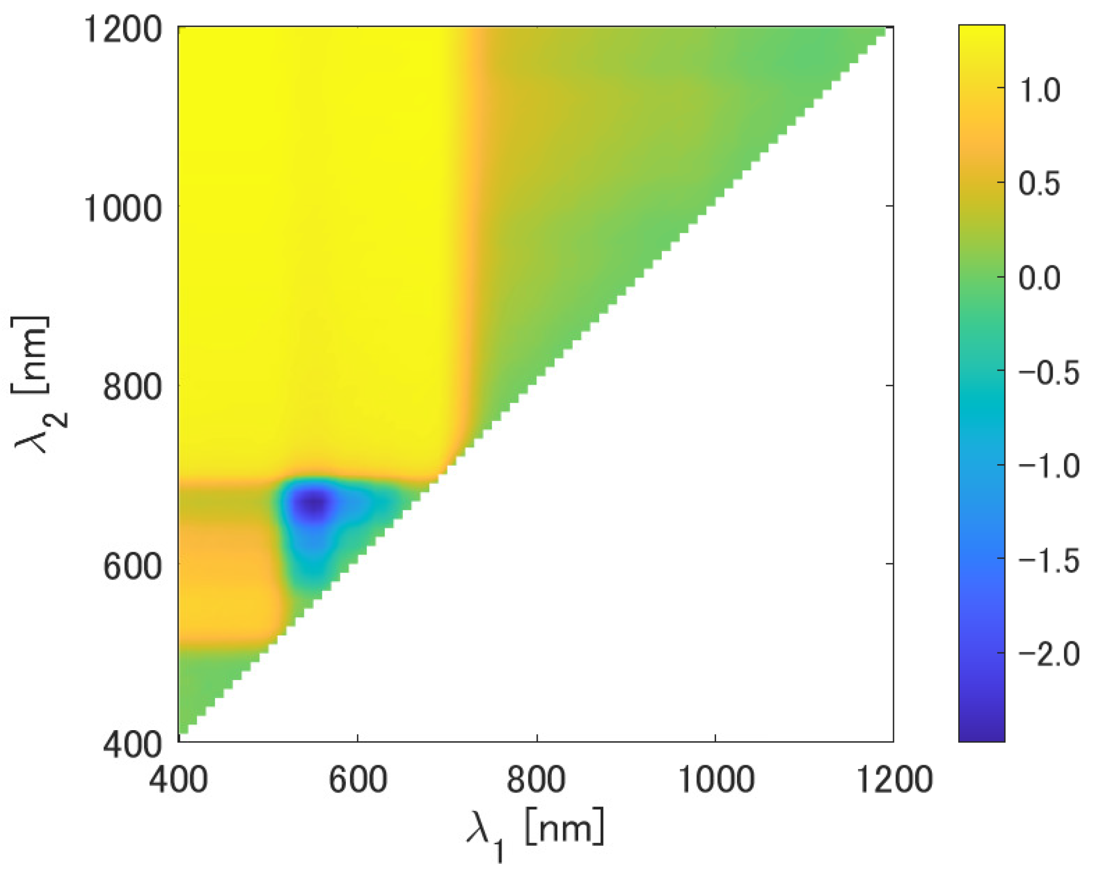
Figure 2 depicts the typical variation patterns of as a function of and . The value of is greater than 1.0 for the combinations visible as and NIR as . Specifically, these wavelength combinations are located in the upper-left region of Figure 2; and range from 400 nm to 710 nm and from 720 nm to 1200 nm, respectively. On the contrary, the value of is negative, with a relatively larger magnitude within a limited region indicated in blue at the lower left. This small region of wavelengths represents the combinations of green as and red as . For these two distinct regions of the subspace, the factor k strongly affects the error reduction. Meanwhile, for the upper-right region and near the lower-left corner of the subspace, the value of is scattered around zero. This result implies that the effect of factor k on the error reduction is relatively less significant than in the two aforementioned regions. These trends shown in Figure 2 are common to all the cases considered in the present study.

Figure 2.
as a function of and .
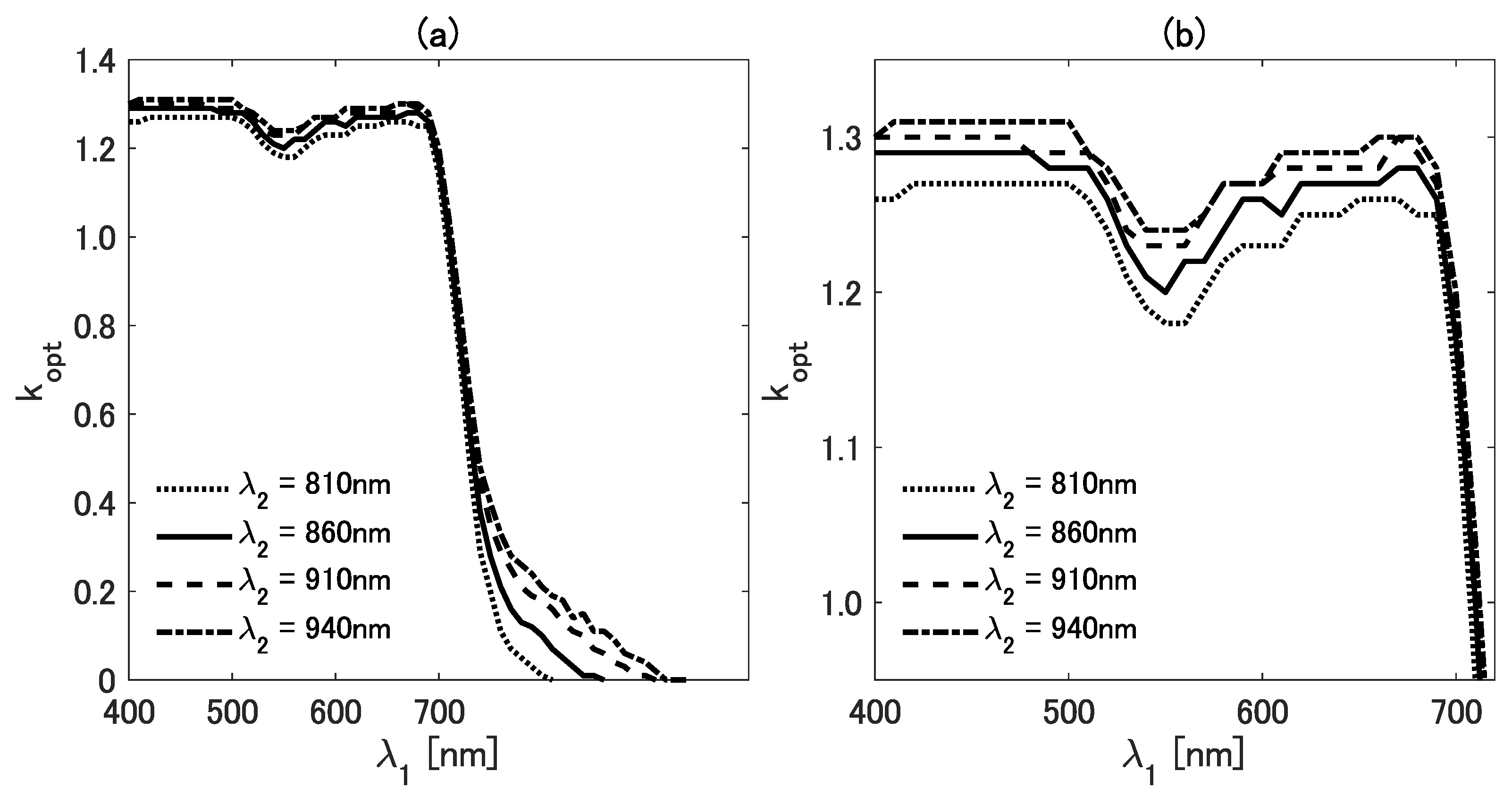
To observe the details of the variations, we plot the cross-section of the figure. Figure 3a,b show as a function of for four different values of (810, 860, 910, and 940 nm). In Figure 3a, the variations of are shown within the range from 400 to 930 nm. To further investigate the details of the differences in the visible region, we plot the results for shorter than 700 nm in Figure 3b. The values of vary from 1.2 to 1.4 when is shorter than 700 nm; it then decreases sharply at 700 nm and approaches zero as increases.
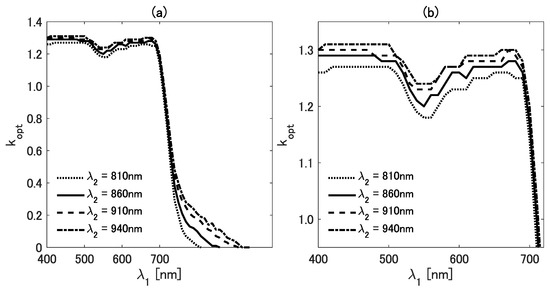
Figure 3.
(a) The value of as a function of for four wavelengths (810, 860, 910, and 940 nm). (b) Enlarged view of (a) in the range from 400 to 700 nm.
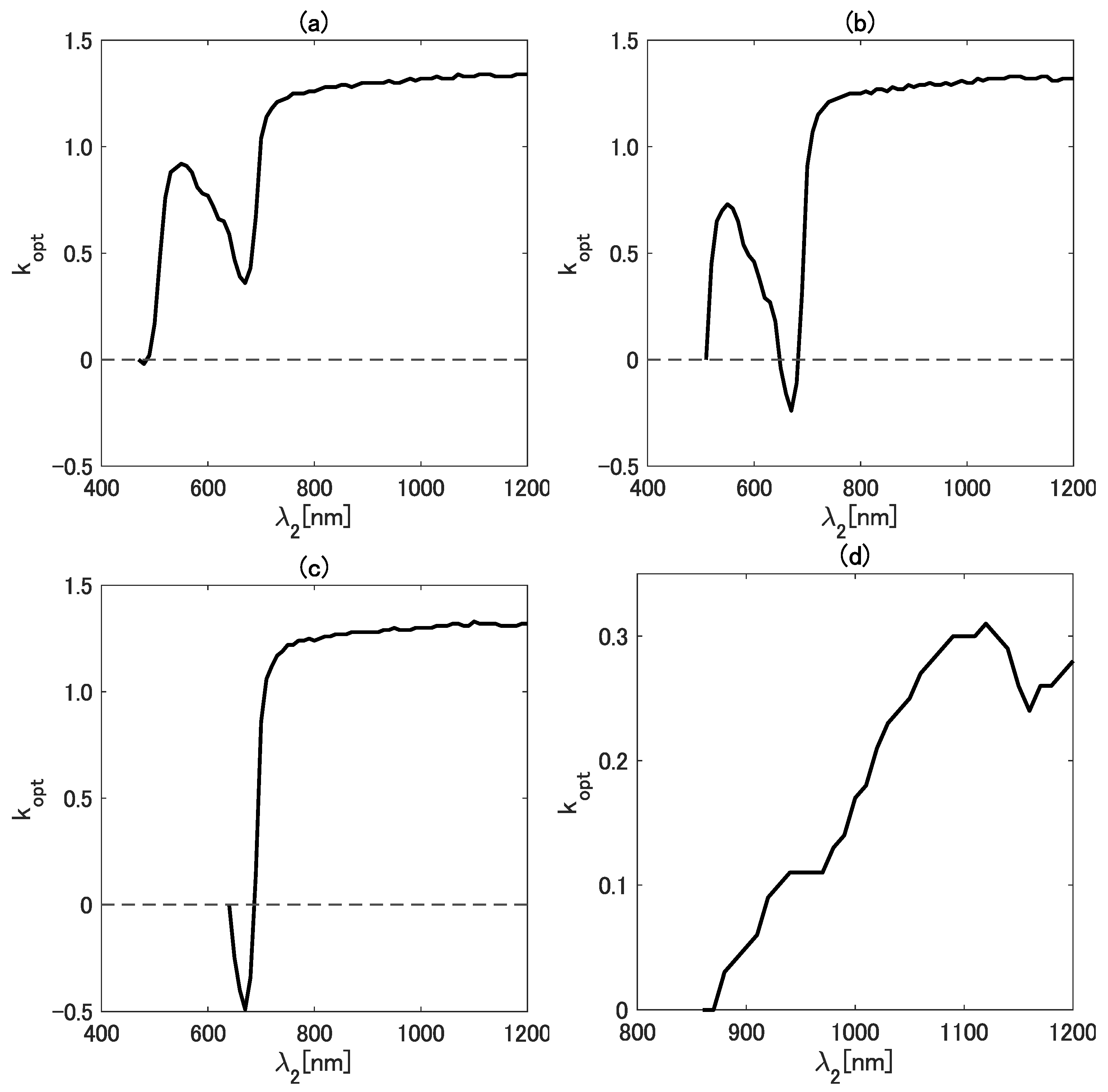
As the next step of the analysis, we referred to a band configuration of an existing satellite sensor. For this purpose, we focused on a new-generation geostationary satellite, Himawari-8 [46]. We applied the band configuration of the Advanced Himawari Imager (AHI) to investigate the behavior of in greater detail to meet the needs of this emerging field of study [42,47,48,49,50,51,52]. Figure 4a–d show as a function of for four wavelengths ((a) 470, (b) 510, (c) 640, and (d) 860 nm). Notably, was assigned as the horizontal axis in this case. The wavelengths chosen for correspond to the visible-to-NIR bands of the AHI.
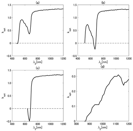
Figure 4.
The value of as a function of for four wavelengths ((a) 470, (b) 510, (c) 640, and (d) 860 nm).
In general, the variation patterns of as a function of show a local minimum and/or maximum in the four cases. Regarding the range, the value of falls between and 1.4 when is in the visible wavelength region. On the contrary, varies in a relatively smaller range (from 0.0 to 0.35) when corresponds to the NIR band (Figure 4). A local maximum and minimum were found in the results in Figure 4 for the case of nm. The local maximum is 0.92 at a wavelength near 550 nm, and the local minimum is 0.36 near 670 nm. Similarly, the local maximum and minimum for the case of nm were found at approximately the same wavelengths as in the case of nm. Interestingly, no local maximum was observed in the case of nm. Although both a local maximum and minimum were observed in the case of nm, their locations differ substantially from those in the other three cases. From these results, special caution is needed when the wavelengths (or bands) from both NIR regions are combined.
Several aspects of the variation of can be explained from the spectral shape of the TOC reflectance. One example is the value of when the TOC reflectance of is greater than that of . Such a case occurs when and are chosen from the visible and NIR bands, respectively. For example, Figure 5a,b show the TOC reflectance spectra for various LAI values with the bright and the dark soils, respectively. In the figure, the reflectance spectra for the visible bands are much smaller than those for the NIR bands, as expected. In this case, the value of becomes greater than 1.0. On the contrary, is expected to be smaller than 1.0 or even a negative value when the TOC reflectance of is smaller than that of . Furthermore, the value of tends to be nearly zero when the TOC reflectances of the two wavelengths are chosen from a similar wavelength region. When we chose the two wavelengths from a similar region, the vegetation isoline tended to be linear. Because the higher-order interaction term does not need to be included to obtain a linear relationship, the value of results in a small-magnitude value to minimize the correction term of the isoline equation. Note also that the fundamentals of the error reduction mechanism of the asymmetric-order vegetation isoline equation were described in [13].
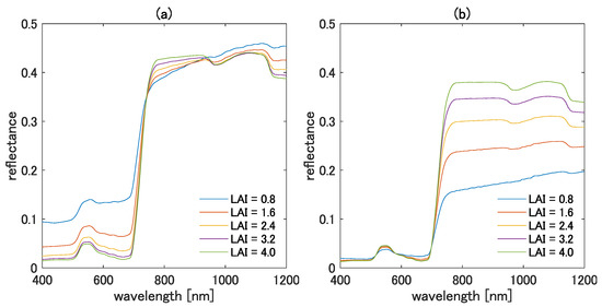
Figure 5.
Simulated TOC reflectance spectra for various LAI values with (a) bright soil and (b) dark soil.
4.2. Accuracy of the Three Vegetation Isolines
In this subsection, we focus on evaluating the accuracy of the three vegetation isoline equations. Recall that the three forms of isolines are denoted by the first-order, the asymmetric-order, and the optimized asymmetric-order vegetation isoline equations. Comparisons of the accuracy were based on the arithmetic mean of computed from the 216 simulations corresponding to different conditions for each wavelength pair.
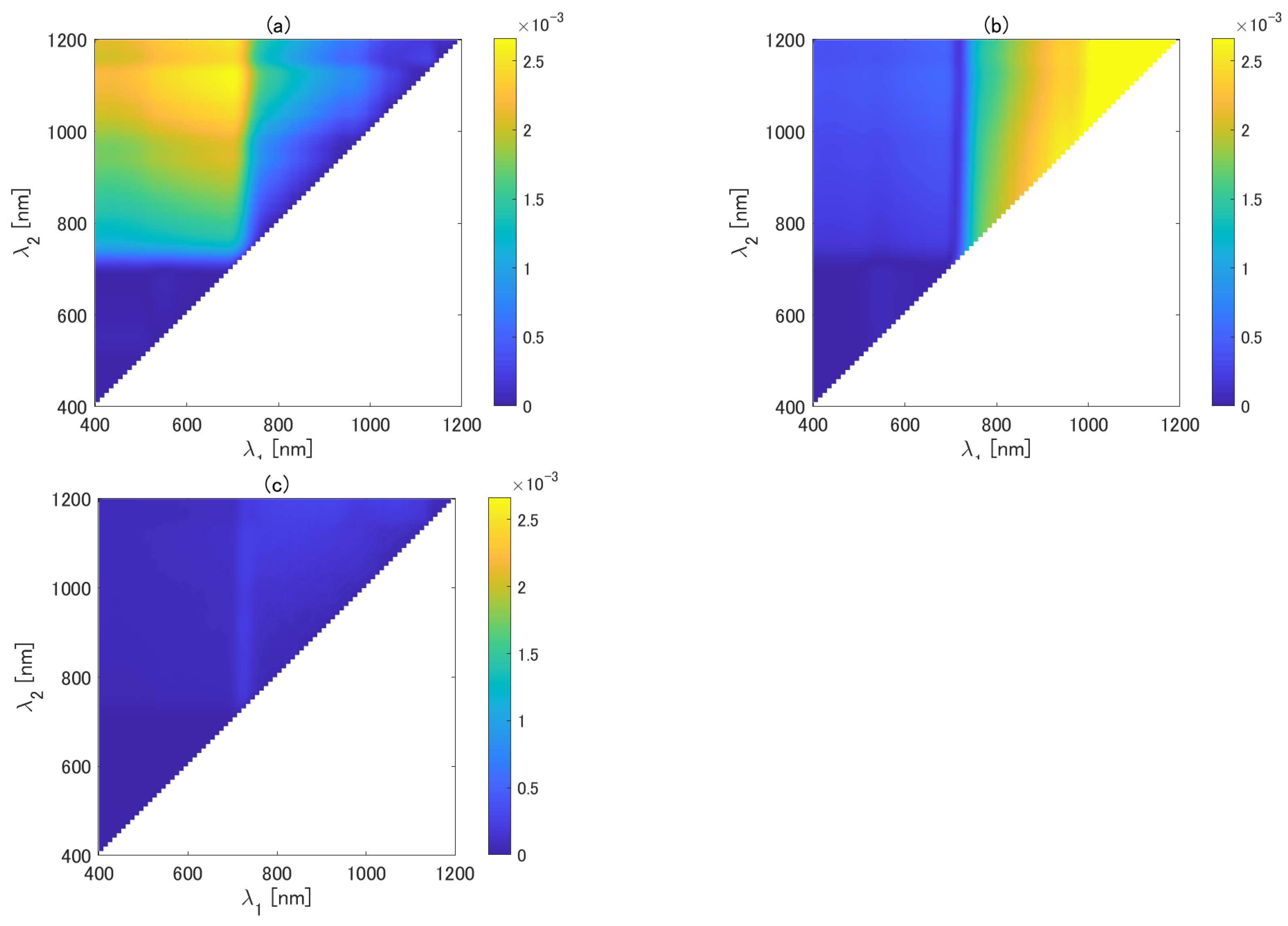
Figure 6 shows the mean epsilon as a function of and for the first-order, the asymmetric-order, and the optimized asymmetric-order isolines (Figure 6a–c). The mean epsilon of the asymmetric-order vegetation isoline is smaller than the first-order vegetation isoline when is chosen from the range between 400 and 710 nm and is chosen from the range between 710 and 1200 nm. By contrast, the mean epsilon of the asymmetric-order vegetation isoline is greater than that of the first-order vegetation isoline in the case where both and are chosen from the NIR range from 720 to 1200 nm. The mean epsilon of the asymmetric-order isoline is similar to that of the first-order isoline when both and are chosen from the visible range (400–700 nm). The optimized asymmetric-order vegetation isoline resulted in a much smaller value of the mean epsilon, which is mostly less than 0.001 for all the regions. The results show the superiority of the optimized asymmetric-order vegetation isoline over the other two isolines.

Figure 6.
Mean epsilon for (a) first-order, (b) asymmetric-order, and (c) optimized asymmetric-order isoline equations as a function of and .
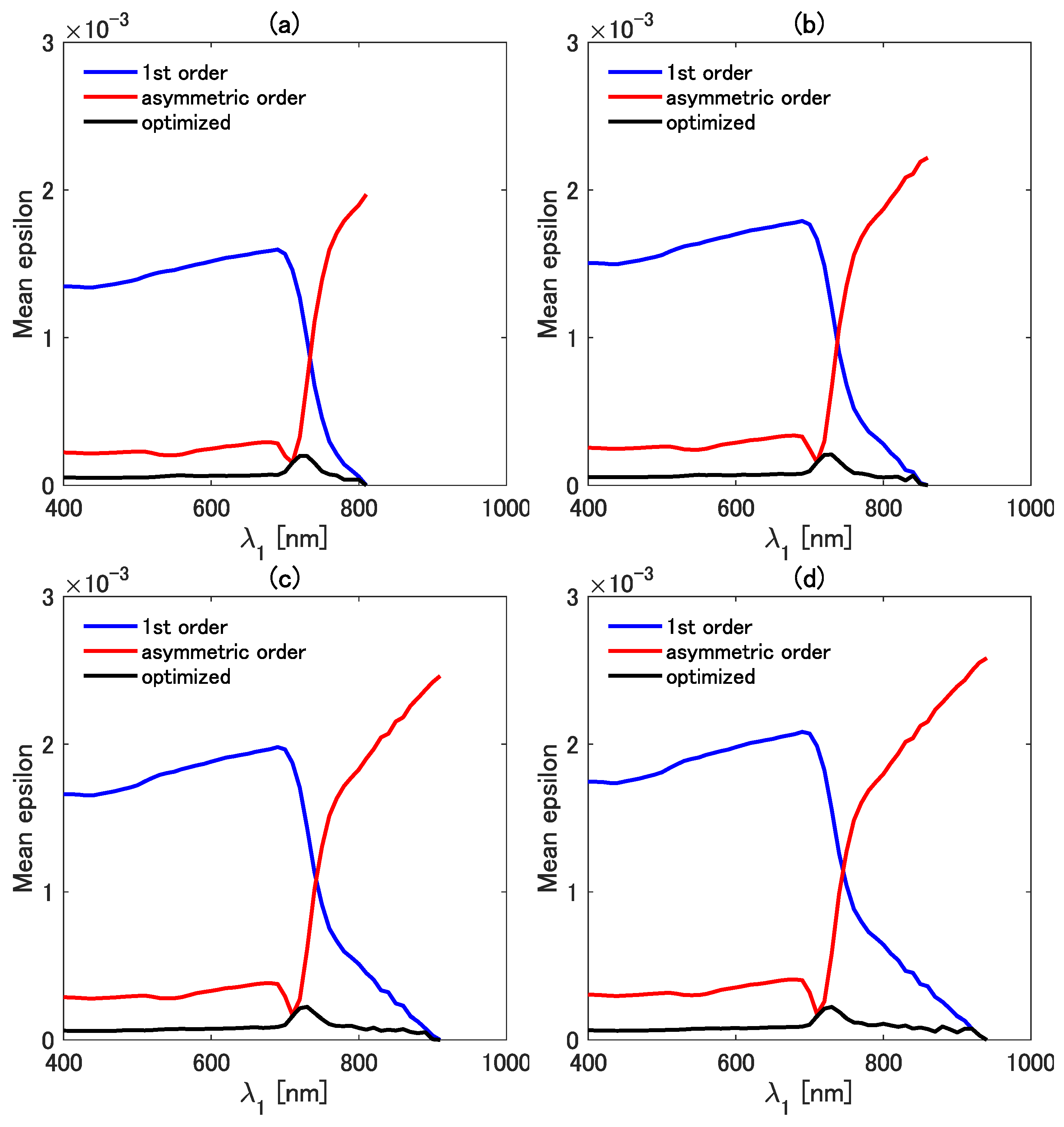
The mean epsilons of the three isolines were directly compared in detail as a function of while was fixed at 810 (Figure 7a), 860 (Figure 7b), 910 (Figure 7c), and 940 nm (Figure 7d). The mean epsilon of the first-order isoline is mostly greater than those of the other two isolines when is less than ∼700 nm for all four cases of . The error in the first-order vegetation isoline, however, decreases with the decreasing difference between and . The mean epsilon of the first-order isoline becomes smaller than that of the asymmetric-order isoline when is greater than ∼750 nm. The mean epsilon of the asymmetric-order vegetation isoline becomes (2.0–3.0) for nm, but the mean epsilon increases rapidly for nm. This result indicates that the correction term introduced in the asymmetric-order isoline makes the error even larger than that of the simplest isoline equation. This error deterioration in the asymmetric-order isoline is improved by introducing the factor k. The optimized asymmetric-order vegetation isoline results in the smallest values of the mean epsilon for all the investigated wavelength pair combinations. These results indicate that the accuracy of the three types of isolines heavily depends on the selected wavelength combination, which implies the importance of the optimization factor k. Importantly, however, the value of k should be set appropriately for each wavelength pair to reduce the error.

Figure 7.
Comparisons of the mean epsilon among the first-order, the asymmetric-order, and the optimized asymmetric-order isolines as a function of at four fixed values of : (a) 810 nm, (b) 860 nm, (c) 910 nm, and (d) 940 nm.
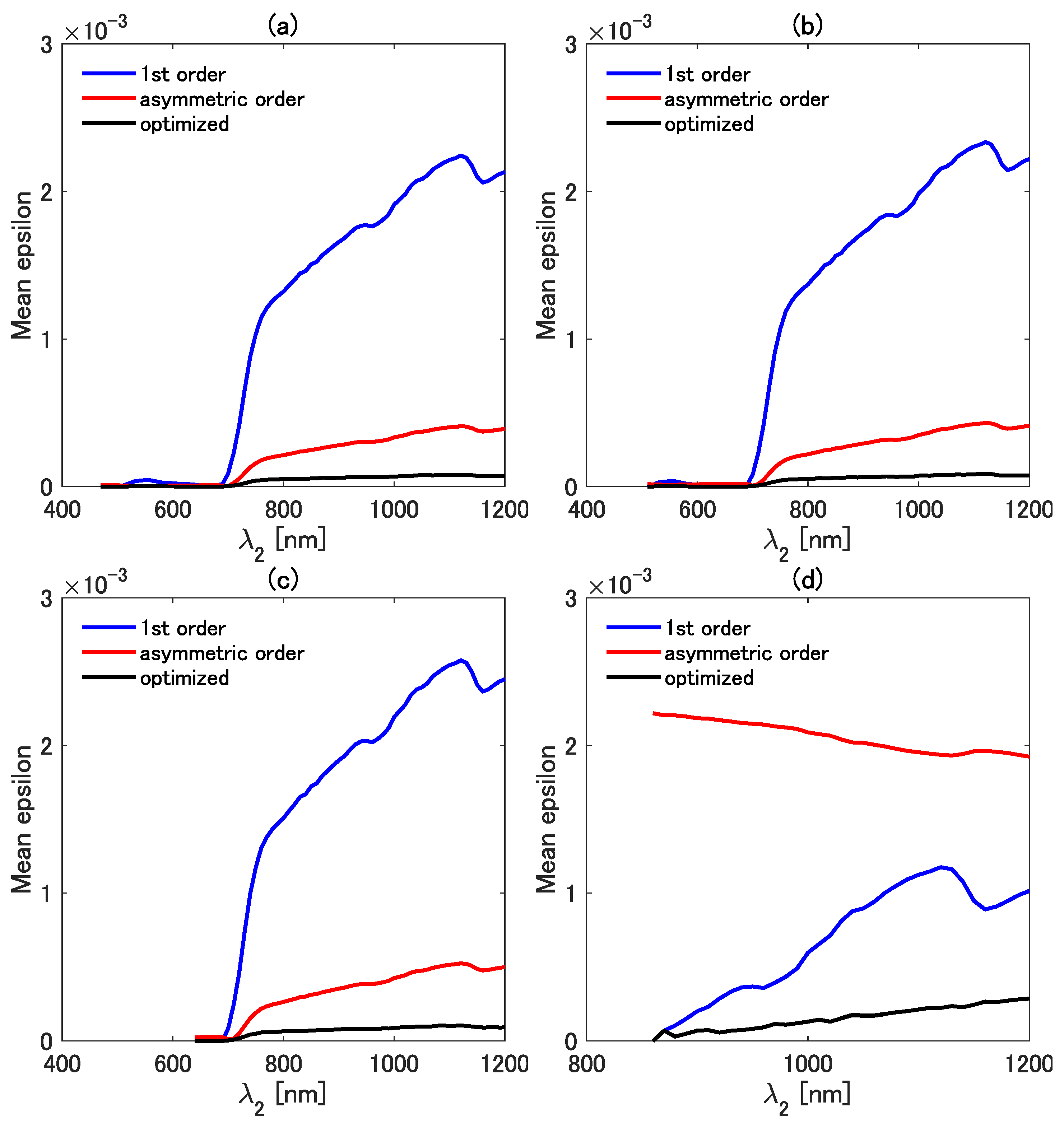
Similar comparisons were made for the mean epsilon of the three types of isolines. Figure 8a–d show a plot of the mean epsilon as a function of at four fixed values of . The value of was fixed at 470 (Figure 8a), 510 (Figure 8b), 640 (Figure 8c), and 860 nm (Figure 8d) in the four cases. The mean epsilon of all three isolines is close to zero in the range less than 700 nm, except for the result shown in Figure 8d, which is the case of nm. By contrast, the mean epsilon shows increasing trends when is greater than 700 nm. Overall, the mean epsilon of the first-order isoline is the greatest among the mean epsilons of the three isolines. The mean epsilon of the asymmetric-order isoline equation, however, becomes the largest in the case of nm (Figure 8d). This result also indicates the need for special caution when choosing the wavelength pair. The results in Figure 7 and Figure 8 imply that the first-order isoline equation could be more accurate than the asymmetric-order isoline equation in the case of some specific wavelength pairs. The reason for this somewhat unexpected result is carefully investigated in the next subsection.
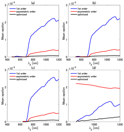
Figure 8.
Comparisons of the mean epsilon among the first-order, the asymmetric-order, and the optimized asymmetric-order isolines as a function of at four fixed values of : (a) 470 nm, (b) 510 nm, (c) 640 nm, and (d) 860 nm.
4.3. Influence of the Higher-Order Interaction Terms Demonstrated in the Reflectance Subspace
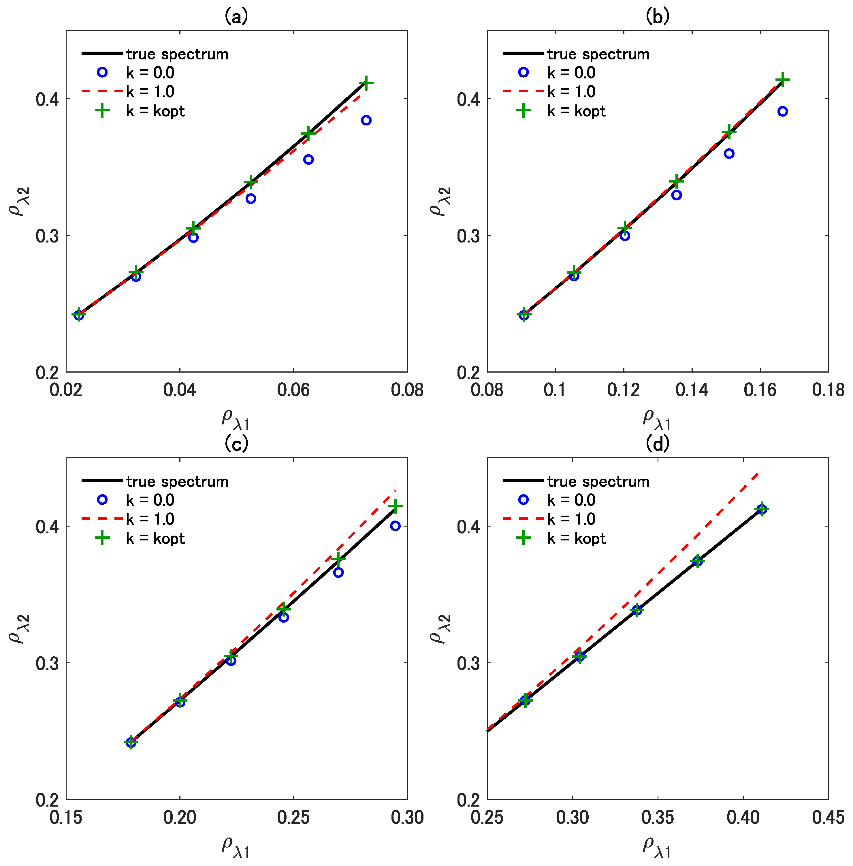
Figure 9 shows the true vegetation isoline and the spectra predicted by the three vegetation isoline equations plotted in the reflectance subspace. The wavelength for was fixed at 860 nm, whereas was varied among four discrete values: (a) 690 nm, (b) 710 nm, (c) 730 nm, and (d) 850 nm, covering from the red edge to the NIR region. Note that the last selected in Figure 9d is close to ; the difference between the two wavelengths is only 10 nm. This choice was made on the basis of the results in Figure 7b, which shows an interesting behavior of the first-order and the asymmetric-order isolines. The values for the LAI and FVC were fixed during the simulation at 1.6 and 1.0, respectively.

Figure 9.
Scatter plot of true spectra and the three variants of isoline equations in the reflectance subspace. The wavelength was fixed at 860 nm, whereas was selected from (a) 690 nm, (b) 710 nm, (c) 730 nm, and (d) 850 nm ( minus 10).
In Figure 9, the first-order, the asymmetric-order, and the optimized asymmetric-order isolines are indicated by blue circles, a red dashed line, and green crosses, respectively. In Figure 9a, the asymmetric-order isoline (red dashed line) is closer to the true isoline (black solid line), clearly indicating that the accuracy of the asymmetric-order vegetation isoline is greater than that of the first-order vegetation isoline. The asymmetric-order isoline in Figure 9b is even closer to the true one compared with that in Figure 9a. Interestingly, the superiority of the asymmetric-order isoline over the first-order isoline is inconsistent. For example, in Figure 9c, the spectra approximated by the asymmetric-order isoline (red dashed line) exceed the true isoline (black solid line), and the distance between the true isoline and the asymmetric-order isoline is almost identical to the distance between the true isoline and the first-order isoline (blue circles). The distance between the true isoline and the asymmetric-order isoline becomes even larger in Figure 9d. The first-order isoline obviously accurately describes the true isoline in the case of Figure 9d, indicating that the influence of the last term of the asymmetric-order isoline adversely affects the accuracy in this case. This problem in the asymmetric-order isoline has been dramatically improved by the introduction of the optimization factor k (the optimized asymmetric-order isoline represented by the green crosses) in all the investigated cases.
To confirm the influence of the higher-order term and its optimization performance represented by the last term in Equation (11), we conducted further error comparisons among the three isolines. Recall that Equation (11) is identical to the first-order vegetation isoline when . When and , Equation (11) results in the asymmetric-order and the optimized asymmetric-order isoline, respectively. Thus, the expression of Equation (11) covers the three types of isoline equations simply because of the selected k factor. We refer to the last term as the “over-correction term” because it is intentionally introduced to overly increase to compensate for the higher-order truncations.
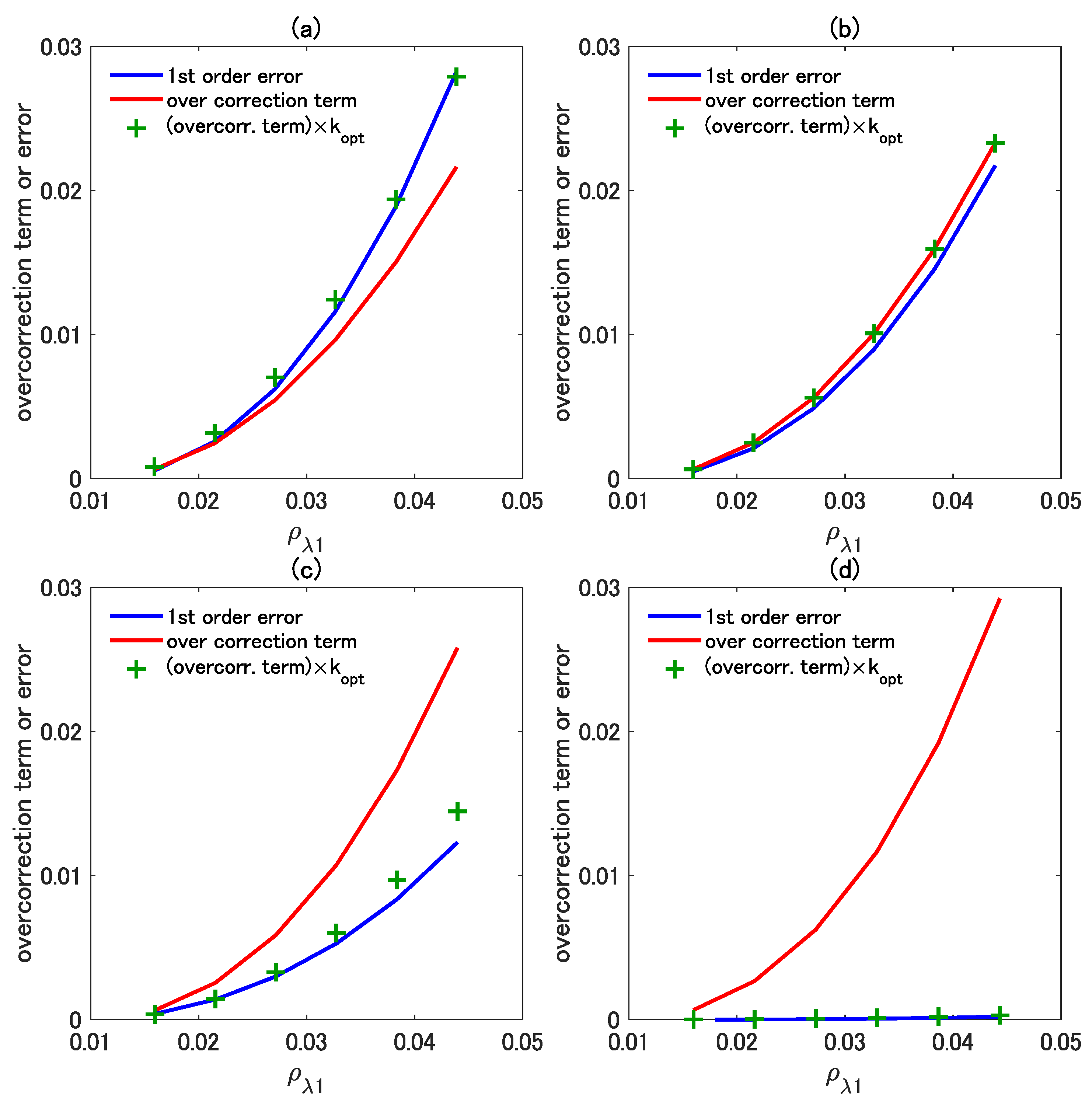
Figure 10a–d show this overcorrection term computed from the last term for the asymmetric-order isoline, (red line), and the optimized higher-order isoline, (green crosses). Furthermore, the error of the first-order isoline, which corresponds to the case of , is shown by the blue line. The combination of the wavelengths, and , is the same as in the case shown in Figure 9. In the cases of Figure 10a,b, the two wavelengths differ to a certain extent; thus, the asymmetric-order isoline shows high accuracy. As evident in the figures, both the green crosses (the optimized asymmetric-order isoline) and the red line (the asymmetric-order isoline) are close to the blue line (the error of the first-order isoline), as we expected. However, when the two wavelengths are similar, the first-order isoline results in better accuracy significantly than the asymmetric-order isoline. This case corresponds to Figure 10c,d, in which the influence of the correction term of the optimized asymmetric-order isoline (green crosses) is much closer to the error of the first-order isoline (blue line) than the correction term of the asymmetric-order isoline (red line). This result implies that the optimized asymmetric-order isoline includes an appropriate value for k and that, because of this appropriate choice of k, the overcorrection term becomes close to the error of the first-order isoline (the truncation error of the isoline) based on the wavelength pair. In summary, the optimized higher-order term nicely minimized the truncation error of the isoline for all combinations of wavelengths, retaining high accuracy irrespective of the wavelength combination.

Figure 10.
Plot of the error in the first-order vegetation isoline equation (blue line) and the over-correction terms of the asymmetric-order vegetation isoline equation (red line) and the adjusted overcorrection term with (green crosses). The wavelength pair of and is the same as in Figure 9. The wavelength was fixed at 860 nm, whereas was selected from (a) 690 nm, (b) 710 nm, (c) 730 nm, and (d) 850 nm ( minus 10).
5. Discussion
The original motivation for developing the isoline formula (the first-order isoline equation) was to analyze the behaviors of the vegetation isoline itself and the spectral VI [10,11]. The derived first-order isoline equation is the simplest among the three isoline equations; hence, it still has an advantage in various analyses. For example, several studies have demonstrated a method that uses the isoline concept for retrieving biophysical parameters such as the FVC and LAI [19,27,53,54,55]. If the first-order isoline equation is used to retrieve these biophysical parameters, the errors caused by the truncation of the higher-order interaction terms will be a major source of error in the retrieved results. For instance, the errors of the first-order isoline are not negligible when it is used for high-accuracy parameter retrievals. This problem should be addressed by retaining its simplicity in the isoline formulation, which was the major challenge of the present research. The initial attempt was to include the higher-order interaction term in a unique manner [13]. The new isoline formula (i.e., the asymmetric-order isoline) can achieve better accuracy than the first-order isoline. However, because the formulation was somewhat unusual (asymmetrical inclusions of the higher-order term), we encountered unexpected behavior in the present study. In particular, the behavior of the errors caused by the choice of the wavelength pair needed to be addressed thoroughly.
In our previous work, we discussed the accuracy of the vegetation isolines for pairs of red and NIR wavelengths by referring to the bands of some existing sensors [14]. For example, when a wavelength pair of 655 and 865 nm is chosen for the red and NIR bands, respectively, we found that the best accuracy was achieved using the optimized asymmetric-order isoline among the three isoline formulas. This study shows that the findings of the previous study remain the same for all the investigated wavelength combinations; the wavelength pair is not limited to the combination of red and NIR wavelengths to support the findings in the previous work [14]. The advantage of the optimized asymmetric-order isoline can also be seen by considering the specifications of the existing hyperspectral sensors. For example, the signal-to-noise ratio (SNR) of EnMAP is 400 in the optical region [38]. The corresponding value of Hyperion is even lower: 144 at 650 nm [56]. Since the reflectance level assumed for the SNR is 0.3 [38], the noise equivalent reflectance becomes 7.5 for EnMAP and 2.1 for Hyperion. From Figure 7a–c, the mean epsilon of the optimized asymmetric-order isoline (black line) is well below the noise equivalent reflectance of those sensors.
On the contrary, the magnitude of the errors in the asymmetric-order isoline is not always smaller than the errors in the first-order isoline, which is a somewhat unexpected result from our previous work [14]. For example, in cases such as those shown in Figure 9c,d, the asymmetric-order isoline showed larger errors than the first-order isoline despite the higher-order interaction term being considered during the derivation. This result implies that special caution is needed to include the higher-order interaction term asymmetrically. Interestingly, the optimization factor k can overcome this difficulty in a wide range of wavelength pairs when the optimum value for k is determined algorithmically. From these results, by using the optimized asymmetric-order isoline, the wavelength region can be extended without exacerbating the errors.
The advantages of the optimized asymmetric-order isoline are improvements in both the accuracy and the flexibility of the wavelength choice. These advantages will lead to better accuracy in parameter retrievals if the first-order isoline is replaced by the optimized asymmetric-order isoline. Suppose that one attempts to retrieve a biophysical parameter using the first-order vegetation isoline equation. Because the error of a retrieved biophysical parameter is expected to be proportional to the error of the isoline equation, an error of nearly 8% [10,11] relative to the retrieved value would be observed when the soil of the canopy background is bright. (This error is due to the relatively larger contribution of the higher-order interaction terms.) This error could be reduced to 1/25 by replacing the first-order isoline by the optimized asymmetric-order isoline. Although the magnitude of the error reduction depends on the wavelength pair, replacement of the isoline may provide a great advantage in various fields of application in which the isoline concept plays an important role [18,33,57,58,59]. This study investigated the errors in the isoline equations within a limited set of parameter settings. This limitation should be noted to consider the results of this study.
6. Conclusions
In our previous work, accuracy assessments were limited to a common pair of red and NIR wavelengths. This limitation was problematic when the isoline concept was used in a broader wavelength region. This study addressed this problem by extending the wavelength range from 400 to 1200 nm. We conducted a set of numerical simulations to characterize the behavior of the three isoline equations. Specifically, the investigation focused on the optimization factor k of the optimized asymmetric-order vegetation isoline.
The factor k introduced in the asymmetric-order isoline equation was simulated under various conditions for each wavelength pair, and its optimum value, , was determined algorithmically for each wavelength pair. The value of was found to strongly depend on the choice of the wavelength pair. In general, three trends were observed in the relationships between the and the wavelength choice. The trends were identified on the basis of the relative differences between the two reflectances. When the reflectance of was greater than that of , the value of tended to be greater than 1. The value of was mostly between 0 and 1 when the reflectances of and were similar. Finally, the value of tended to be less than 0 when the reflectance of was less than that of .
With respect to the accuracy of the three variants of the vegetation isoline, the optimized asymmetric-order isoline equation was the most accurate for all the wavelength pairs investigated in the present study. The asymmetric-order isoline equation, in general, showed better accuracy than the first-order isoline equation; however, this trend did not hold for some wavelength pairs. Specifically, when the reflectances of the two wavelengths were similar, the accuracy of the asymmetric-order isoline equation was worse than that of the first-order isoline equation. This result could have been caused by the effects of the asymmetrical inclusion of the higher-order interaction. This negative influence of the asymmetric term was clarified in the present study. We expect the developed isoline formula to be useful in a wide range of applications involving analytical and numerical tools. The application of the optimized asymmetric-order isoline equation to actual data processing of existing hyperspectral sensors remains undone, which should be considered as a future effort. Further efforts will be needed to facilitate the isoline formula as a practical tool for processing satellite data.
Author Contributions
Conceptualization, M.M. and H.Y.; methodology, M.M., H.Y. and K.O.; software, M.M.; validation, K.O. and H.Y.; formal analysis, M.M., K.O. and H.Y.; investigation, M.M.; resources, M.M. and H.Y.; data curation, M.M.; writing—original draft preparation, M.M.; writing—review and editing, K.O. and H.Y.; visualization, M.M.; supervision, H.Y.; project administration, H.Y.; funding acquisition, H.Y. and K.O. All authors have read and agreed to the published version of the manuscript.
Funding
This research was funded by JSPS KAKENHI Grant Numbers JP20K20487, JP20K12259, and JP20KK0237.
Data Availability Statement
Not applicable.
Conflicts of Interest
The authors declare no conflict of interest.
References
- Zhu, Z.; Bi, J.; Pan, Y.; Ganguly, S.; Anav, A.; Xu, L.; Samanta, A.; Piao, S.; Nemani, R.R.; Myneni, R.B. Global data sets of vegetation leaf area index (LAI) 3g and fraction of photosynthetically active radiation (FPAR) 3g derived from global inventory modeling and mapping studies (GIMMS) normalized difference vegetation index (NDVI3g) for the period 1981 to 2011. Remote Sens. 2013, 5, 927–948. [Google Scholar] [CrossRef] [Green Version]
- Hansen, M.C.; Potapov, P.V.; Moore, R.; Hancher, M.; Turubanova, S.A.; Tyukavina, A.; Thau, D.; Stehman, S.; Goetz, S.J.; Loveland, T.R.; et al. High-resolution global maps of 21st-century forest cover change. Science 2013, 342, 850–853. [Google Scholar] [CrossRef] [PubMed] [Green Version]
- Huete, A.R. A soil-adjusted vegetation index (SAVI). Remote Sens. Environ. 1988, 25, 295–309. [Google Scholar] [CrossRef]
- Baret, F.; Guyot, G.; Major, D. TSAVI: A vegetation index which minimizes soil brightness effects on LAI and APAR estimation. In Proceedings of the 12th Canadian Symposium on Remote Sensing Geoscience and Remote Sensing Symposium, Vancouver, BC, Canada, 10–14 July 1989; Volume 3, pp. 1355–1358. [Google Scholar] [CrossRef]
- Major, D.; Baret, F.; Guyot, G. A ratio vegetation index adjusted for soil brightness. Int. J. Remote Sens. 1990, 11, 727–740. [Google Scholar] [CrossRef]
- Qi, J.; Chehbouni, A.; Huete, A.; Kerr, Y.; Sorooshian, S. A modified soil adjusted vegetation index. Remote Sens. Environ. 1994, 48, 119–126. [Google Scholar] [CrossRef]
- Verstraete, M.M.; Pinty, B. Designing optimal spectral indexes for remote sensing applications. IEEE Trans. Geosci. Remote Sens. 1996, 34, 1254–1265. [Google Scholar] [CrossRef]
- Gilabert, M.; González-Piqueras, J.; Garcıa-Haro, F.; Meliá, J. A generalized soil-adjusted vegetation index. Remote Sens. Environ. 2002, 82, 303–310. [Google Scholar] [CrossRef]
- Jiang, Z.; Huete, A.R.; Didan, K.; Miura, T. Development of a two-band enhanced vegetation index without a blue band. Remote Sens. Environ. 2008, 112, 3833–3845. [Google Scholar] [CrossRef]
- Yoshioka, H.; Huete, A.R.; Miura, T. Derivation of vegetation isoline equations in red-NIR reflectance space. IEEE Trans. Geosci. Remote Sens. 2000, 38, 838–848. [Google Scholar] [CrossRef]
- Yoshioka, H.; Miura, T.; Huete, A.; Ganapol, B.D. Analysis of vegetation isolines in red-NIR reflectance space. Remote Sens. Environ. 2000, 74, 313–326. [Google Scholar] [CrossRef]
- Yoshioka, H. Vegetation isoline equations for an atmosphere-canopy-soil system. IEEE Trans. Geosci. Remote Sens. 2004, 42, 166–175. [Google Scholar] [CrossRef]
- Miura, M.; Obata, K.; Yoshioka, H. Vegetation isoline equations with first-and second-order interaction terms for modeling a canopy-soil system of layers in the red and near-infrared reflectance space. J. App. Remote Sens. 2015, 9, 095987. [Google Scholar] [CrossRef] [Green Version]
- Miura, M.; Obata, K.; Taniguchi, K.; Yoshioka, H. Improved accuracy of the asymmetric second-order vegetation isoline equation over the red–NIR reflectance space. Sensors 2017, 17, 450. [Google Scholar] [CrossRef] [PubMed] [Green Version]
- Miura, M.; Obata, K.; Taniguchi, K.; Yoshioka, H. Optimization technique of asymmetric-order vegetation isoline equations. In Proceedings of the 2017 IEEE International Geoscience and Remote Sensing Symposium (IGARSS), Fort Worth, TX, USA, 23–28 July 2017; pp. 2923–2926. [Google Scholar] [CrossRef]
- Yoshioka, H.; Miura, T.; Demattê, J.A.; Batchily, K.; Huete, A.R. Derivation of soil line influence on two-band vegetation indices and vegetation isolines. Remote Sens. 2009, 1, 842–857. [Google Scholar] [CrossRef] [Green Version]
- Yoshioka, H.; Miura, T.; Demattê, J.A.; Batchily, K.; Huete, A.R. Soil line influences on two-band vegetation indices and vegetation isolines: A numerical study. Remote Sens. 2010, 2, 545–561. [Google Scholar] [CrossRef] [Green Version]
- Fan, X.; Liu, Y. Multisensor Normalized Difference Vegetation Index Intercalibration: A comprehensive overview of the causes of and solutions for multisensor differences. IEEE Geosci. Remote Sens. Mag. 2018, 6, 23–45. [Google Scholar] [CrossRef]
- Sun, Y.; Lu, L.; Liu, Y. Inversion of the leaf area index of rice fields using vegetation isoline patterns considering the fraction of vegetation cover. Int. J. Remote Sens. 2021, 42, 1688–1712. [Google Scholar] [CrossRef]
- Baret, F.; Guyot, G. Potentials and limits of vegetation indices for LAI and APAR assessment. Remote Sens. Environ. 1991, 35, 161–173. [Google Scholar] [CrossRef]
- Jackson, R.; Pinter, P., Jr.; Reginato, R.; Idso, S. Hand-Held Radiometry: A Set of Notes Developed for Use at the Workshop of Hand-Held Radiometry; Technical Report; Agricultural Research (Western Region), Science and Education Administration, U.S. Department of Agriculture: Phoenix, AZ, USA, 1980.
- Kimes, D.S.; Norman, J.M.; Walthall, C.L. Modeling the radiant transfers of sparse vegetation canopies. IEEE Trans. Geosci. Remote Sens. 1985, GE-23, 695–704. [Google Scholar] [CrossRef]
- Sellers, P.J. Canopy reflectance, photosynthesis and transpiration. Int. J. Remote Sens. 1985, 6, 1335–1372. [Google Scholar] [CrossRef]
- Huete, A.; Jackson, R. Suitability of spectral indices for evaluating vegetation characteristics on arid rangelands. Remote Sens. Environ. 1987, 23, 213–232, IN1–IN8. [Google Scholar] [CrossRef]
- Gobron, N.; Pinty, B.; Verstraete, M.M.; Widlowski, J.L. Advanced vegetation indices optimized for up-coming sensors: Design, performance, and applications. IEEE Trans. Geosci. Remote. Sens. 2000, 38, 2489–2505. [Google Scholar] [CrossRef]
- Yoshioka, H.; Yamamoto, H.; Miura, T. Use of an isoline-based inversion technique to retrieve a leaf area index for inter-sensor calibration of spectral vegetation index. In Proceedings of the IEEE International Geoscience and Remote Sensing Symposium, IGARSS’02, Toronto, ON, Canada, 24–28 June 2002; Volume 3, pp. 1639–1641. [Google Scholar] [CrossRef]
- Kallel, A.; Le Hégarat-Mascle, S.; Ottlé, C.; Hubert-Moy, L. Determination of vegetation cover fraction by inversion of a four-parameter model based on isoline parametrization. Remote Sens. Environ. 2007, 111, 553–566. [Google Scholar] [CrossRef]
- Okuda, K.; Taniguchi, K.; Miura, M.; Obata, K.; Yoshioka, H. Application of vegetation isoline equations for simultaneous retrieval of leaf area index and leaf chlorophyll content using reflectance of red edge band. In Remote Sensing and Modeling of Ecosystems for Sustainability XIII; International Society for Optics and Photonics: Bellingham, WA, USA, 2016; Volume 9975, p. 99750C. [Google Scholar] [CrossRef]
- Yoshioka, H.; Miura, T.; Huete, A.R. An isoline-based translation technique of spectral vegetation index using EO-1 Hyperion data. IEEE Trans. Geosci. Remote Sens. 2003, 41, 1363–1372. [Google Scholar] [CrossRef]
- Yoshioka, H.; Miura, T.; Yamamoto, H. Analytical relationships of inter-sensor vegetation indices based on the theory of vegetation isoline. In Proceedings of the IEEE International Geoscience and Remote Sensing Symposium, IGARSS’05, Seoul, Korea, 29 July 2005; Volume 6, pp. 4164–4167. [Google Scholar] [CrossRef]
- Yoshioka, H.; Miura, T.; Obata, K. Derivation of relationships between spectral vegetation indices from multiple sensors based on vegetation isolines. Remote Sens. 2012, 4, 583–597. [Google Scholar] [CrossRef] [Green Version]
- Obata, K.; Miura, T.; Yoshioka, H.; Huete, A.R. Derivation of a MODIS-compatible enhanced vegetation index from visible infrared imaging radiometer suite spectral reflectances using vegetation isoline equations. J. App. Remote Sens. 2013, 7, 073467. [Google Scholar] [CrossRef] [Green Version]
- Fan, X.; Liu, Y. A generalized model for intersensor NDVI calibration and its comparison with regression approaches. IEEE Trans. Geosci. Remote Sens. 2016, 55, 1842–1852. [Google Scholar] [CrossRef]
- Iwasaki, A.; Ohgi, N.; Tanii, J.; Kawashima, T.; Inada, H. Hyperspectral Imager Suite (HISUI)-Japanese hyper-multi spectral radiometer. In Proceedings of the 2011 IEEE International Geoscience and Remote Sensing Symposium, Vancouver, BC, Canada, 24–29 July 2011; pp. 1025–1028. [Google Scholar] [CrossRef]
- Obata, K.; Tsuchida, S.; Nagatani, I.; Yamamoto, H.; Kouyama, T.; Yamada, Y.; Yamaguchi, Y.; Ishii, J. An overview of ISS HISUI hyperspectral imager radiometric calibration. In Proceedings of the 2016 IEEE International Geoscience and Remote Sensing Symposium (IGARSS), Beijing, China, 10–15 July 2016; pp. 1924–1927. [Google Scholar] [CrossRef]
- Matsunaga, T.; Iwasaki, A.; Tsuchida, S.; Iwao, K.; Nakamura, R.; Yamamoto, H.; Kato, S.; Obata, K.; Kashimura, O.; Tanii, J.; et al. HISUI status toward FY2019 launch. In Proceedings of the IGARSS 2018-2018 IEEE International Geoscience and Remote Sensing Symposium, Valencia, Spain, 22–27 July 2018; pp. 160–163. [Google Scholar] [CrossRef]
- Obata, K. Sensitivity analysis method for spectral band adjustment between hyperspectral sensors: A case study using the CLARREO Pathfinder and HISUI. Remote Sens. 2019, 11, 1367. [Google Scholar] [CrossRef] [Green Version]
- Guanter, L.; Kaufmann, H.; Segl, K.; Foerster, S.; Rogass, C.; Chabrillat, S.; Kuester, T.; Hollstein, A.; Rossner, G.; Chlebek, C.; et al. The EnMAP Spaceborne Imaging Spectroscopy Mission for Earth Observation. Remote Sens. 2015, 7, 8830–8857. [Google Scholar] [CrossRef] [Green Version]
- Alonso, K.; Bachmann, M.; Burch, K.; Carmona, E.; Cerra, D.; de los Reyes, R.; Dietrich, D.; Heiden, U.; Hölderlin, A.; Ickes, J.; et al. Data Products, Quality and Validation of the DLR Earth Sensing Imaging Spectrometer (DESIS). Sensors 2019, 19, 4471. [Google Scholar] [CrossRef] [Green Version]
- Vangi, E.; D’Amico, G.; Francini, S.; Giannetti, F.; Lasserre, B.; Marchetti, M.; Chirici, G. The New Hyperspectral Satellite PRISMA: Imagery for Forest Types Discrimination. Sensors 2021, 21, 1182. [Google Scholar] [CrossRef] [PubMed]
- Baret, F.; Jacquemoud, S.; Hanocq, J. The soil line concept in remote sensing. Remote Sens. Rev. 1993, 7, 65–82. [Google Scholar] [CrossRef]
- Obata, K.; Taniguchi, K.; Matsuoka, M.; Yoshioka, H. Development and Demonstration of a Method for GEO-to-LEO NDVI Transformation. Remote Sens. 2021, 13, 4085. [Google Scholar] [CrossRef]
- Jacquemoud, S.; Verhoef, W.; Baret, F.; Bacour, C.; Zarco-Tejada, P.J.; Asner, G.P.; François, C.; Ustin, S.L. PROSPECT+ SAIL models: A review of use for vegetation characterization. Remote Sens. Environ. 2009, 113, S56–S66. [Google Scholar] [CrossRef]
- Jacquemoud, S.; Baret, F. PROSPECT: A model of leaf optical properties spectra. Remote Sens. Environ. 1990, 34, 75–91. [Google Scholar] [CrossRef]
- Verhoef, W. Light scattering by leaf layers with application to canopy reflectance modeling: The SAIL model. Remote Sens. Environ. 1984, 16, 125–141. [Google Scholar] [CrossRef] [Green Version]
- Bessho, K.; Date, K.; Hayashi, M.; Ikeda, A.; Imai, T.; Inoue, H.; Kumagai, Y.; Miyakawa, T.; Murata, H.; Ohno, T.; et al. An introduction to Himawari-8/9—Japan’s new-generation geostationary meteorological satellites. J. Meteorol. Soc. Japan. Ser. II 2016, 94, 151–183. [Google Scholar] [CrossRef] [Green Version]
- Adachi, Y.; Kikuchi, R.; Matsuoka, M.; Ichii, K.; Yoshioka, H. Reflectance comparison between Himawari-8 AHI and Terra MODIS over a forest of Shikoku region. In Land Surface and Cryosphere Remote Sensing IV; International Society for Optics and Photonics: Bellingham, WA, USA, 2018; Volume 10777, p. 1077715. [Google Scholar] [CrossRef]
- Miura, T.; Nagai, S.; Takeuchi, M.; Ichii, K.; Yoshioka, H. Improved characterisation of vegetation and land surface seasonal dynamics in central Japan with Himawari-8 hypertemporal data. Sci. Rep. 2019, 9, 15692. [Google Scholar] [CrossRef] [Green Version]
- Wang, W.; Li, S.; Hashimoto, H.; Takenaka, H.; Higuchi, A.; Kalluri, S.; Nemani, R. An introduction to the Geostationary-NASA Earth Exchange (GeoNEX) Products: 1. Top-of-atmosphere reflectance and brightness temperature. Remote Sens. 2020, 12, 1267. [Google Scholar] [CrossRef] [Green Version]
- Obata, K.; Yoshioka, H. A Simple Algorithm for Deriving an NDVI-Based Index Compatible between GEO and LEO Sensors: Capabilities and Limitations in Japan. Remote Sens. 2020, 12, 2417. [Google Scholar] [CrossRef]
- Xiao, J.; Fisher, J.B.; Hashimoto, H.; Ichii, K.; Parazoo, N.C. Emerging satellite observations for diurnal cycling of ecosystem processes. Nat. Plants 2021, 7, 877–887. [Google Scholar] [CrossRef] [PubMed]
- Hashimoto, H.; Wang, W.; Dungan, J.L.; Li, S.; Michaelis, A.R.; Takenaka, H.; Higuchi, A.; Myneni, R.B.; Nemani, R.R. New generation geostationary satellite observations support seasonality in greenness of the Amazon evergreen forests. Nat. Commun. 2021, 12, 684. [Google Scholar] [CrossRef] [PubMed]
- Zhao, H.S.; Zhu, X.C.; Li, C.; Wei, Y.; Zhao, G.X.; Jiang, Y.M. Improving the accuracy of the hyperspectral model for apple canopy water content prediction using the equidistant sampling method. Sci. Rep. 2017, 7, 11192. [Google Scholar] [CrossRef] [PubMed] [Green Version]
- Ali, A.M.; Darvishzadeh, R.; Skidmore, A.; Heurich, M.; Paganini, M.; Heiden, U.; Mücher, S. Evaluating prediction models for mapping canopy chlorophyll content across biomes. Remote Sens. 2020, 12, 1788. [Google Scholar] [CrossRef]
- Ali, A.M.; Darvishzadeh, R.; Skidmore, A.; Gara, T.W.; O’ Connor, B.; Roeoesli, C.; Heurich, M.; Paganini, M. Comparing methods for mapping canopy chlorophyll content in a mixed mountain forest using Sentinel-2 data. Int. J. Appl. Earth Obs. Geoinf. 2020, 87, 102037. [Google Scholar] [CrossRef]
- Folkman, M.A.; Pearlman, J.; Liao, L.B.; Jarecke, P.J. EO-1/Hyperion hyperspectral imager design, development, characterization, and calibration. In Hyperspectral Remote Sensing of the Land and Atmosphere; Smith, W.L., Yasuoka, Y., Eds.; International Society for Optics and Photonics, SPIE: Bellingham, WA, USA, 2001; Volume 4151, pp. 40–51. [Google Scholar] [CrossRef]
- Donohue, R.J.; Roderick, M.L.; McVicar, T.R. Deriving consistent long-term vegetation information from AVHRR reflectance data using a cover-triangle-based framework. Remote Sens. Environ. 2008, 112, 2938–2949. [Google Scholar] [CrossRef]
- Zhang, X.; Tan, B.; Yu, Y. Interannual variations and trends in global land surface phenology derived from enhanced vegetation index during 1982–2010. Int. J. Biometeorol. 2014, 58, 547–564. [Google Scholar] [CrossRef] [Green Version]
- Fan, X.; Liu, Y. A comparison of NDVI intercalibration methods. Int. J. Remote Sens. 2017, 38, 5273–5290. [Google Scholar] [CrossRef]
Publisher’s Note: MDPI stays neutral with regard to jurisdictional claims in published maps and institutional affiliations. |
© 2022 by the authors. Licensee MDPI, Basel, Switzerland. This article is an open access article distributed under the terms and conditions of the Creative Commons Attribution (CC BY) license (https://creativecommons.org/licenses/by/4.0/).


