OpenHSI: A Complete Open-Source Hyperspectral Imaging Solution for Everyone

Abstract

OpenHSI is an initiative to lower the barriers of entry and bring compact pushbroom hyperspectral imaging spectrometers to a wider audience. We present an open-source optical design that can be replicated with readily available commercial-off-the-shelf components, and an open-source software platform openhsi that simplifies the process of capturing calibrated hyperspectral datacubes. Some of the features that the software stack provides include: an ISO 19115-2 metadata editor, wavelength calibration, a fast smile correction method, radiance conversion, atmospheric correction using 6SV (an open-source radiative transfer code), and empirical line calibration. A pipeline was developed to customise the desired processing and make openhsi practical for real-time use. We used the OpenHSI optical design and software stack successfully in the field and verified the performance using calibration tarpaulins. By providing all the tools needed to collect documented hyperspectral datasets, our work empowers practitioners who may not have the financial or technical capability to operate commercial hyperspectral imagers, and opens the door for applications in new problem domains.

1. Introduction

Microscale hyperspectral imaging spectrometers capture reflectance measurements in the visible–near-infrared spectrum, usually from 400 to 1000 nm—the detection range of silicon CMOS sensors [1]. The spatial and spectral information can be used to classify biophysical features on the Earth’s surface and has found applications in agriculture [2,3], forestry and environmental management [4,5], water and maritime resource management [6,7], and the detection of iron oxides [8]. The smaller size and weight enables more diverse methods of deployment, such as drones and CubeSats, compared to larger HyperSpectral Imagers (HSI) such as NASA’s AVIRIS [9] and Hyperion [10], and HyVista’s HyMap [11].

Recent developments in portable field-deployable HSIs have focused on making the technology cheaper, smaller, and lightweight for do-it-yourself applications ranging from crop monitoring [12] to monitoring water quality [13]. Existing solutions come in two main flavours that make trade-offs between spatial and spectral resolution and speed of capture. While pushbroom HSIs can be capable of nanometre spectral resolution, the device needs to be scanned across the desired scene and the resulting datacube can contain unwanted motion artefacts. On the other hand, snapshot HSIs can have no moving parts but generally must make a trade-off between spectral or spatial resolution, and deal with the offset between pixels and bands. Most microscale solutions use only commercial-off-the-shelf (COTS) components, but some use photolithography to produce custom lenses [14]. A custom machined enclosure is common, whereas some are 3D printed.

Popular solutions implemented in the literature revolve mainly around pushbroom and snapshot modes of operation, although there are others, such as whiskbroom and spatiospectral. For large airborne applications, pushbroom sensors have been ‘standard’ for years and the miniaturisation for small-scale deployment on lightweight platforms is a recent development. A great summary of the different spectral sensor types can be found in [15].

In a pushbroom scanner, a line of spatial information is recorded per frame, with each pixel on this line spectrally dispersed to obtain spectral information. To obtain 2D spatial information, this line is scanned across a target through motion. This could be from a moving platform such as an aircraft, satellite, UAV, or a rotation stage. Handheld platforms such as a motorised selfie stick provide a convenient method for urban greening monitoring [16]. Furthermore, pushbrooms can be mounted in a stationary position and items can be analysed under a conveyor belt or by sliding an object through the field of view, as demonstrated by [17]. One example where a datacube was captured by a stationary HSI involved rotary mirrors to generate the necessary motion [18]; however, the trade-off was a nonportable design which was limited to a lab setting.

An alternative to pushbroom is to use a snapshot imager which captures a datacube in one frame. The downside is a lower spectral resolution limited by the array of filters on the focal plane, but this method does not incur motion artefacts. A particularly thin package involving a prism mirror array was developed by [14]. However, their design required photolithography to create custom lenses and other components, making it an expensive option to manufacture. A benefit of this different design was the possibility for high-magnification objective lenses to be mounted and for datacubes to be produced without motion artefacts. Ref. [14] used this approach to image pollen. All these implementations rely on a Charge Coupled Device (CCD) Camera, with most opting for a monochrome sensor since it is sensitive to the whole visible spectrum. The snapshot HSI presented in [19] used a CCD sensor with a Bayer filter and anti-aliasing filter. The downside was a large Full Width Half Maximum (FWHM) of >20 nm, especially towards the red. This contrasted with the $\approx 6$ nm spectral resolution available in commercial pushbroom sensors such as the Headwall Micro-Hyperspec [15].

The masses of the preceding microscale HSIs were typically below the mass of state-of-the-art pushbroom sensors for UAVs, which weigh between 0.5 and 4 kg (usually ≈1 kg; [15]). The exceptions were some designs that used motorised parts or a machined enclosure, which added significantly to the mass budget and limited use to the lab settings, large drones, and fixed wing aircraft. For the dispersive element, gratings (either reflection or transmission) and prisms are used (or a combination of both).

For open-source software, [20] included a smile correction package based on the same optical design described in [21]. However, the algorithm presented does not lend itself to fast real-time processing and the software is not readily extensible.

The reality is that building and calibrating a compact HSI still requires substantial technical expertise, which can place hyperspectral technology out of reach for many practitioners. In the spirit of removing such barriers, OpenHSI is a pushbroom HSI composed entirely of COTS optical components with a 3D-printed enclosure and optical improvements over similar published designs such as [21]. A pushbroom design allows OpenHSI to retain high spectral resolution and we quantify the Signal to Noise Ratio (SNR) performance in Section 2. The calibration and operations of OpenHSI are supported by an open-source Python library (hereby called openhsi) complete with documentation and tutorials. At the time of writing, there is not yet a complete software stack to facilitate the collection of radiometrically corrected hyperspectral datasets with optimisations for real-time processing on development compute platforms. In short, OpenHSI is a project that aims to solve these problems, by providing a detailed hardware design and a modular software library that are both open-source and are intended to lower the barriers to building, calibrating, and operating an HSI.

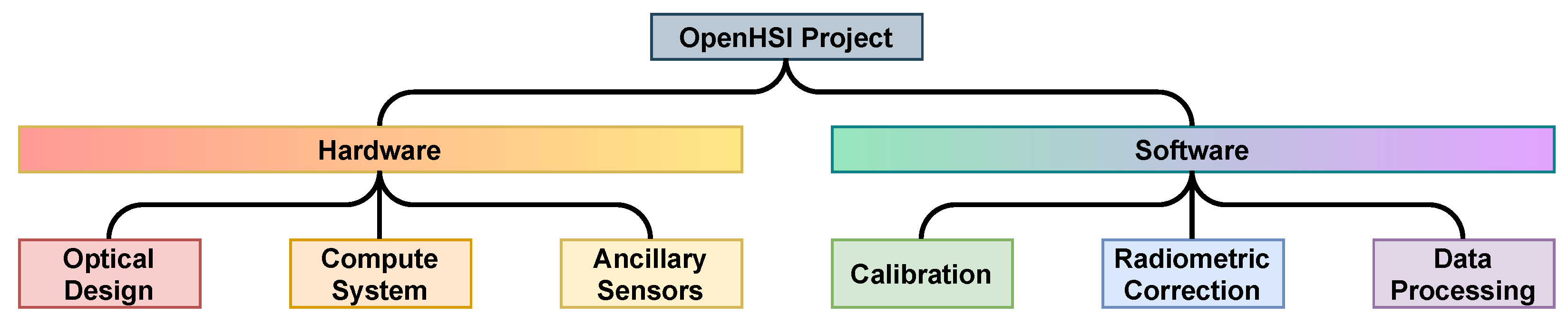
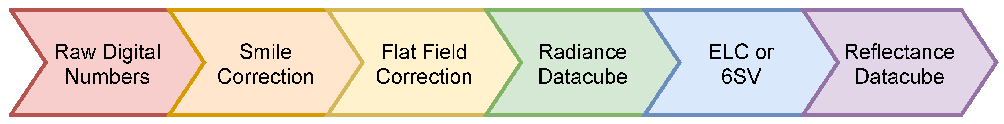
The general structure of this paper follows the components in Figure 1 from left to right, separated broadly into hardware and software. We present a validation of the OpenHSI camera and software in Section 7, through airborne collected data and an analysis of the reflectance estimates of calibration tarpaulins, and then conclude the paper.

2. Optical Design

To evaluate the performance of the HSI presented in [21], we simulated the optical design in Zemax OpticStudio. The optical system is separated into three basic stages, called the camera lens, collimator system, and the field lens. The camera lens is a proprietary design, but was simulated using a Zemax encrypted Blackbox. However, in the case of the field lens, no Blackbox was available. To approximate the field lens, we use an equivalent paraxial (perfect) lens. The performance showed significant chromatic aberration, which resulted in image quality degradation away from the central 550 nm wavelength. This was due to the use of non-achromatic lenses in the collimator. By substituting the primary lens in the collimator with an achromatic lens of the same focal length, we find that the image quality is improved and made more consistent across the detector array’s field of view. This is illustrated by the spot diagrams in Figure 2.

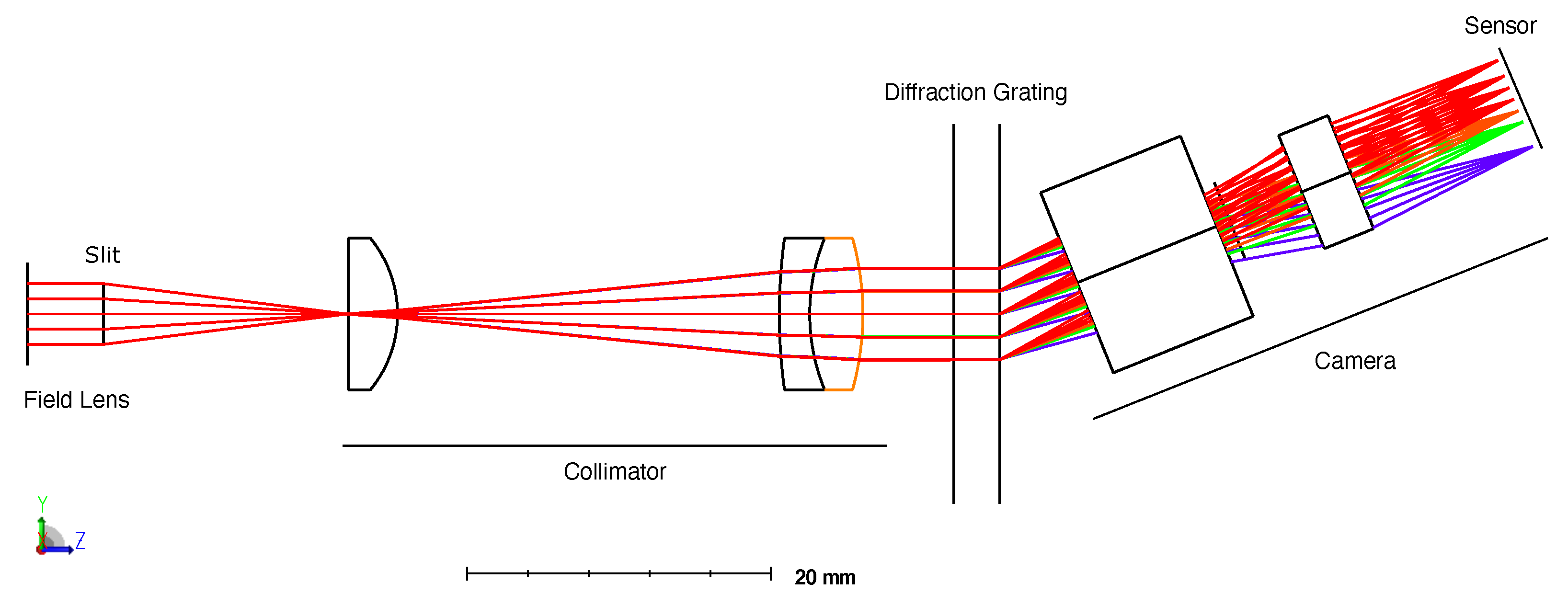
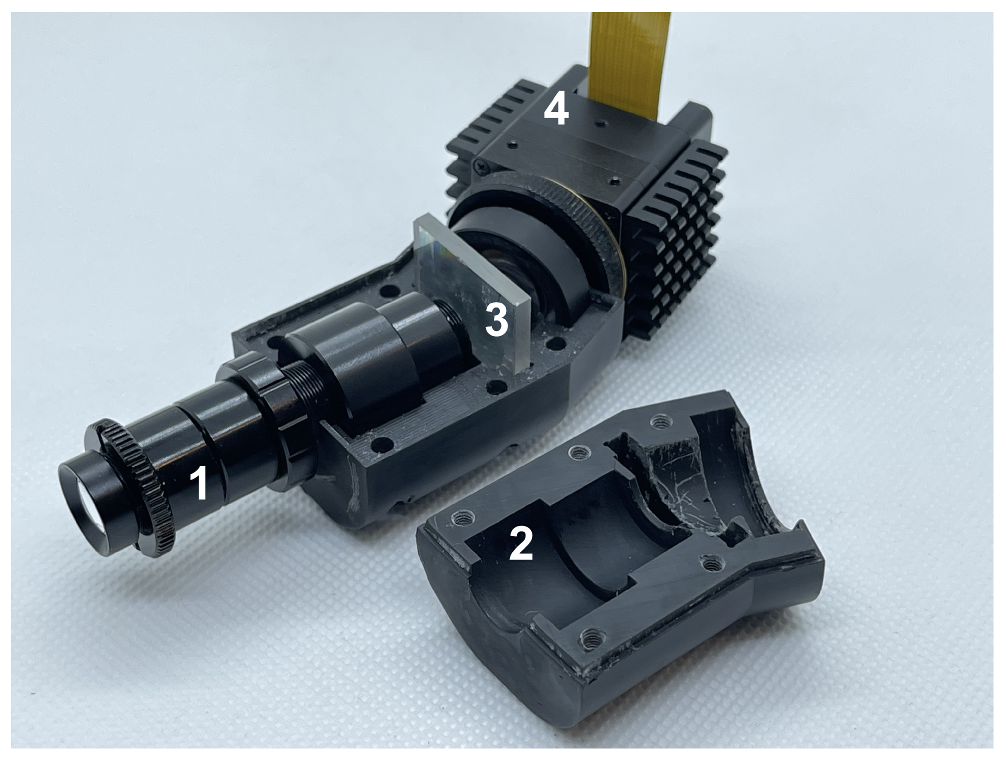
The component layout of OpenHSI is shown in Figure 3, with the angle set to match a transmission grating with a line density of 600 lines/mm and a 28.7° blaze angle, so as to minimise losses. We used a monochrome XIMEA MX031MG-SY2 machine vision camera with the Sony IMX252 sensor package, which has an 2064 × 1544 (3.1 MP) array of 3.45 µm pixels. A camera with this sensor was chosen primarily for its relatively high frame rates, while also having a low noise readout and a global shutter. In our implementation, the camera was connected to an NVIDIA Jetson board through a PCIe link, allowing for a fast base frame rate of 233 FPS with 12 bit data. Each frame was windowed to 2064 (spectral) × 772 (spatial) and the pixels were binned 1 × 2, to better match the OpenHSI optical footprint. The longer dimension was used for the spectra, which was then later binned into spectral bands in software.

Due to the chosen lenses being unsuited near and below 400 nm and a lower solar irradiance in the blue compared to the rest of the visible spectrum, we shifted the centre wavelength towards the red compared to [21]. The usable range was 450–800 nm, with vignetting occurring for wavelengths outside this range. In practice, we found that we were able to use a slightly larger range during data collection (400–830 nm after calibration). We used a 3 mm × 25 µm slit and placed the camera at the first diffraction order of the grating—the reason for the 19.36° bend. The spectral range was also limited by the overlap of the first and second spectral orders. A transmission grating was chosen over a prism due to its dispersion properties and its smaller size and mass—although a prism will not have overlapping orders.

The major COTS components used in OpenHSI are listed in

Table 1. Parts list.

Item	Description	Part Number	Supplier
1	Field Lens	#83-107	Edmund Optics
2	Slit	A-SLIT-3/8-DISC-25	Lenox Laser
3	Collimator Lens 1	#63-519	Edmund Optics
4	Collimator Lens 2	#63-720	Edmund Optics
4	Grating	#49-580	Edmund Optics
5	Camera Lens	#56-776	Edmund Optics
6	XIMEA Detector	MX031MG-SY
7	3D-Printed Enclosure

. There are also a few smaller components, such as a lens tube, slit mount, threaded inserts, and spacers. The enclosure design files can be found in the GitHub repository https://github.com/openhsi (accessed on 5 April 2022) and can be 3D printed. We were able to keep the mass of OpenHSI down to 119 g by using a small detector and a 3D-printed enclosure, making it an option for those with smaller portable platforms. A summary of the characteristics that OpenHSI achieves is given in

Table 2. OpenHSI characteristics.

Dimensions	116 mm × 46 mm × 35 mm
Mass	119 g
Bands	108 (4 nm bands; can be reconfigured)
Working F/#	4
Ground sample distance	5 cm at 120 m altitude (0.42 mrad)
Spectral range	400–830 nm (with some vignetting)
Field of view	10.6°

.

2.1. Optics Enclosure

Conforming to the aim of making OpenHSI inexpensive and quick to prototype, we chose to follow [21] in 3D printing the enclosure but redesigned it from scratch, informed by our experience with other 3D-printed spectrograph housings—for example, in [22]. We tested two printing methods, the first using fused deposition of ABS using a Stratasys UPrint SE Plus and finally using a Formlabs Form3 SLA printer (which cures a photosensitive resin). The SLA parts offered higher precision, allowing us to directly print threads in the parts, and were chosen for later enclosures.

Despite being less sturdy than a machined metal housing, additive manufacturing has several advantages, including quick prototyping and allowing lighter designs that lend themselves to do-it-yourself applications. Printed parts also allow some geometries and configurations that would be very expensive or impossible to machine. Our final assembly with all optical components and detector installed came to 119 g.

The enclosure shown in Figure 4 was printed in two halves, allowing components to be placed within before the two halves are joined. The two halves are joined using a lip and grove feature, and pulled together using M2.5 thread holes integrated in the print, clamping the lens tube assembly in place. The enclosure design also integrates 4 (2 top, 2 bottom) M3 brass inserts as mounting points for more flexible integration in a scanning platform. These mounting holes also allow the camera to be fixed to a compute device.

There are a few versions of the open-source CAD model for use with specific sensors and one design intended for integration with generic C-mount cameras allowing for other commercial camera sensors to be easily attached. The camera-specific enclosures have a small platform that grips the camera. We found this very helpful in keeping the detector pixels aligned with the slit by stopping unintentional rotation.

It is important to keep the camera at a temperature within manufacturer specifications to prevent damage and reduce the effect of dark current and hot pixels. For an outdoor application where OpenHSI is to be flown by a drone or fixed wing aircraft, there will be ample airflow to keep the device cool. For indoor applications, we recommend attaching heat sinks or stopping image acquisition when not needed, either by a hardware switch or through software.

2.2. Signal to Noise

For a microscale HSI, one of the trade-offs to achieve a compact size is in the Signal to Noise Ratio (SNR). SNR is a measure of the signal power divided by the noise power and can be a limiting factor in classification quality, as shown, for example, by [23] for mineral classification. What constitutes an acceptable SNR depends on the use case, with large state-of-the-art HSIs capable of SNRs > 500:1 [11]. We calculated the SNR for OpenHSI based on the diffraction efficiency of the grating and the quantum efficiency of the Sony IMX252 CMOS sensor.

Assuming that the dominant source of noise is photon shot noise ${\sigma }_s=\sqrt{S}$, the SNR is given by

$$\mathrm{SNR}\approx S/{\sigma }_s=\sqrt{S},$$

(1)

where the signal

$$S={\eta }_{QE,\lambda }N\Delta t,$$

(2)

${\eta }_{QE,\lambda }$ is the quantum efficiency, N is the number of photons per second, and $\Delta t$ the exposure time. The number of photons per second is then given by the formula [24]

$$N_{\lambda }=L_{\lambda }{\rho }_{\lambda }{\eta }_{opt}{\eta }_{G,\lambda }{\eta }_{QE,\lambda }{A}_d\Delta \lambda \frac{\lambda }{hc}\frac{\pi }{4{(\mathrm{F}/\#)}^2}$$

(3)

where $L_{\lambda }$ is the solar radiance at the Earth’s surface given the geolocation and UTC time, ${\rho }_{\lambda }$ is the surface reflectance, ${\eta }_{opt}$ is the optical transmission efficiency, ${\eta }_{G,\lambda }$ is the diffraction grating efficiency, $A_d$ is the detector area, $\Delta \lambda$ is the FWHM or bandwidth, $\lambda$ is the centre wavelength, and F/# is the F number.

In the SNR plot shown in Figure 5, we assume a constant surface albedo of 30%. The solar radiance at the sensor was estimated using a radiative transfer model (6SV) for a location near Cairns, Queensland, Australia at the time and date when the dataset shown in Section 7 was recorded (around 2 pm local time on 26 May 2021). The solar zenith angle was 43°. More information on the parameters used in 6SV can be found in Section 6.1. The sharp dip at 760 nm is due to the O${}_2$-A absorption band. Part of the reason that OpenHSI has an SNR within 100 s is due to the slit width of 25 µm and the combination of a 10 ms exposure time and choice of 4 nm spectral bands. Without increasing the integration time, which is limited by the desired spatial resolution and the airspeed and altitude for an airborne platform, the SNR can be increased by using a larger slit size and sacrificing some spectral resolution. The spectral binning procedure can be customised and more details can be found in Section 5. Depending on the use case and required real-time processing, a suitable compute system needs to be considered.

3. Compute System

The open-source Python library openhsi currently supports a subset of XIMEA cameras, FLIR cameras, and Lucid cameras connected to an NVIDIA Jetson board or Raspberry Pi4 board through a PCIe bus, USB port, or gigabit ethernet. The level of real-time processing between successive image captures can be specified at initialisation and this impacts the camera frame rate. The additional processing means that the frame rate will be lower than what the exposure time will suggest. This in turn affects the flight speed if square pixels are desired. To speed up processing, most arrays are preallocated and set up as circular buffers to avoid reallocating memory. While testing on a Jetson Xavier AGX board set to 15 W mode, an exposure time of 10 ms corresponded to 75 frames per second (FPS) when processing to binned digital numbers (DNs).

Another cause of latency is the time taken to save a large datacube to disk. Our tests indicate that it takes around 3 s to create and save a 800 MB NetCDF file to an NVMe SSD connected via an M.2 slot. If raw data are desired, a development board with ≥4 GB of RAM is necessary and, even then, at 90 FPS (no binning), one will spend a significant amount of time creating and saving files instead of collecting data.

Since the camera is designed to be mounted to a moving platform, the resulting data will incur motion artefacts that distort the imagery. We also want to geolocate the pixels with GPS coordinates and to measure the humidity during test flights, so as to better calibrate the atmospheric absorption effects in the 6SV correction procedure. For this reason, a GPS device, an IMU, and a combined pressure, humidity, and temperature sensor need to be connected to the compute board. This was done using the 40 pin general purpose input/output (GPIO) header on the Jetson development boards and Raspberry Pi4. Georectification for OpenHSI data will be the topic of an upcoming paper by [25].

Ancillary Sensors

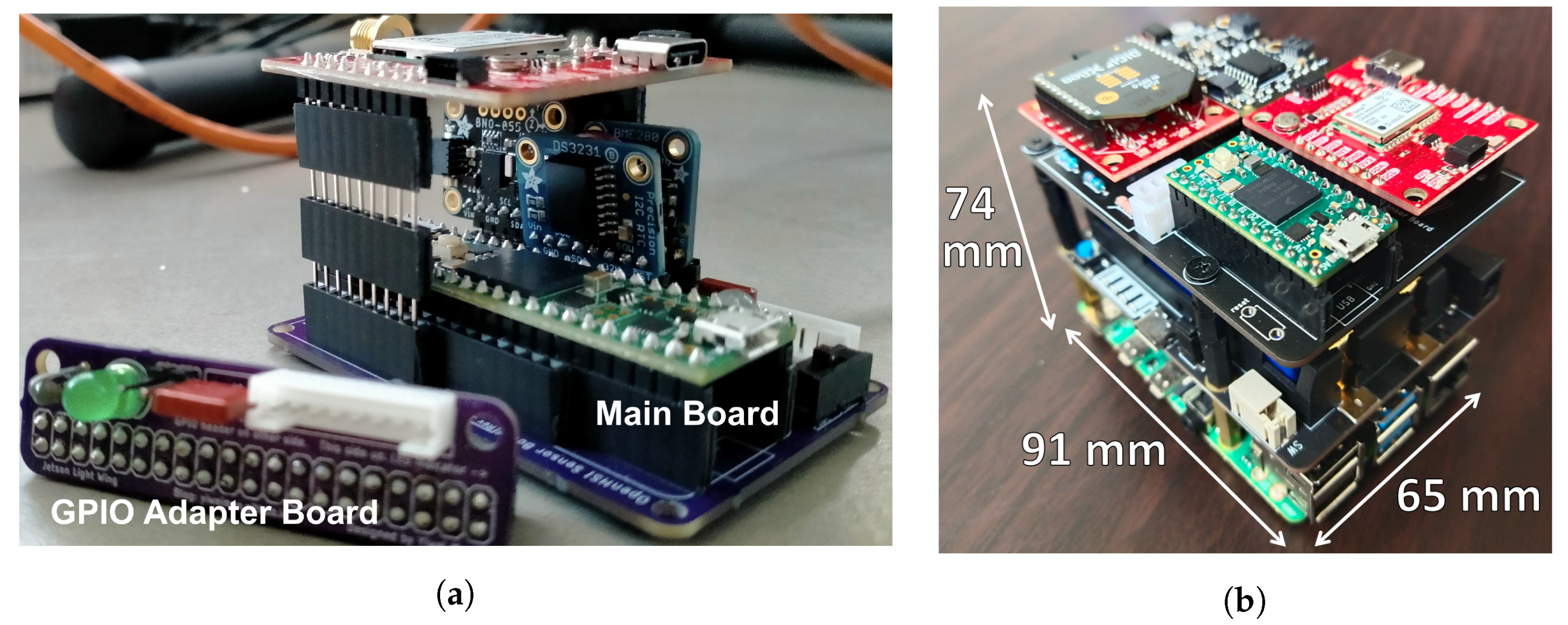
Connected to our Jetson Xavier AGX was a small Printed Circuit Board (PCB), shown in Figure 6a, that facilitated the collection of ancillary sensor data for assisting atmospheric and geometric correction. The sensors include: an IMU (BNO055); a humidity, temperature, and pressure sensor (BME280); a high-precision real-time clock (DS3231), and GPS (GPS NEO M9N). We chose to use a dedicated microcontroller with a real-time clock instead of the Jetson to update each sensor with timestamps. This was to avoid inconsistent timing effects due to the Jetson’s operating system scheduler.

With the ancillary sensors timestamped to the GPS time, the challenge is then to synchronise the data to the camera capture times. Synchronisation can be achieved by reading the GPS pulse per second signal as a GPIO interrupt. However, this required knowledge of the GPS time at the moment of interrupt (which are held in each data packet transmitted) so, instead, we used a more general method by treating each data packet event as a pseudo-interrupt. For each data packet received, we timestamped the system time, and the time offset can be found directly, albeit limited by the serial polling rate. To reduce interference in camera data collection, ancillary sensor data were collected in a separate CPU process. In practice, the timing accuracy achieved was around 1 ms.

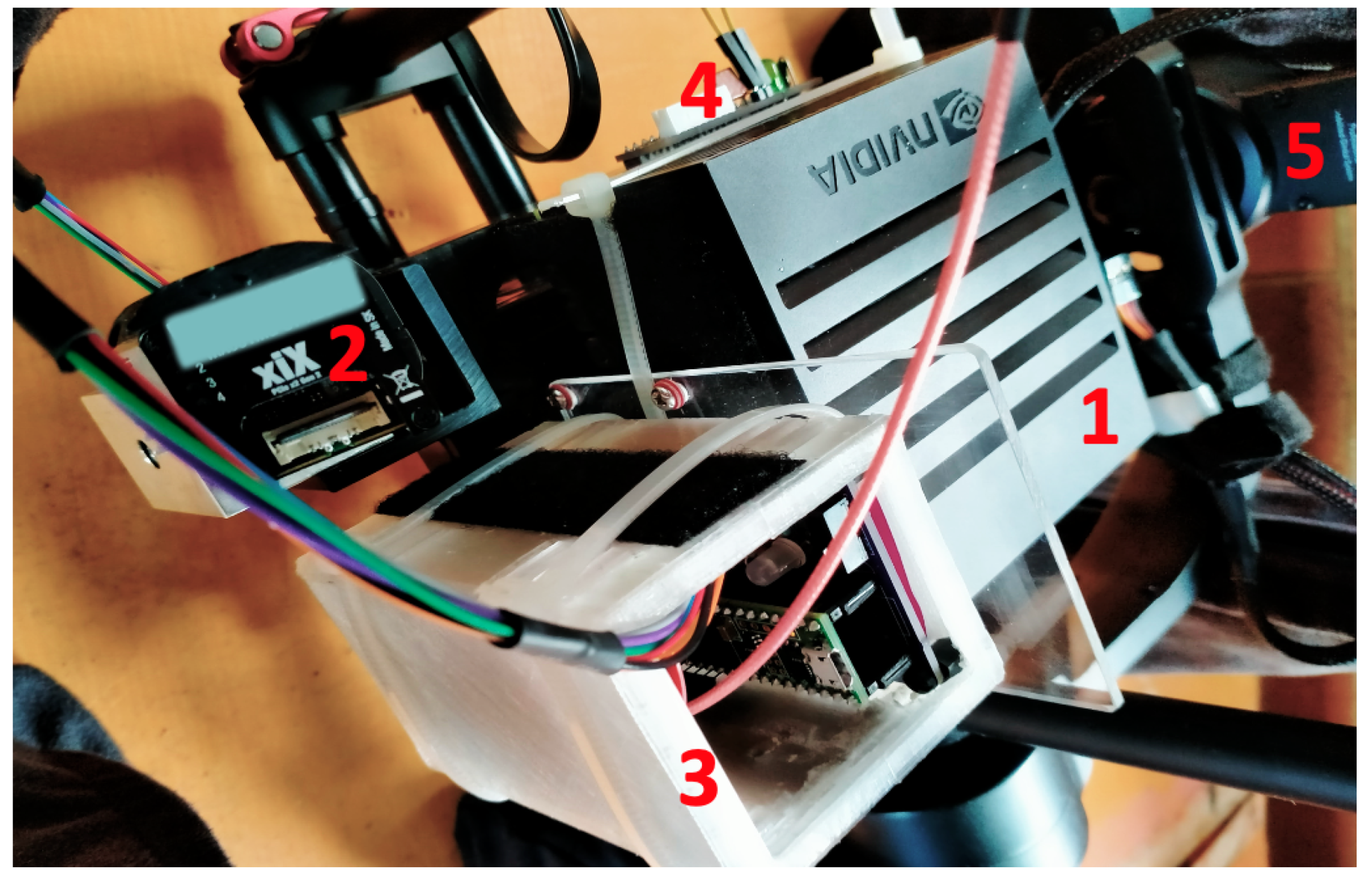
All sensor data were processed at their highest update rate by a Teensy 4.1 microcontroller, which then transferred the data to the Jetson over serial to be stored with the captured datacube. Not all the 40 GPIO pins available were required, so we used a smaller PCB as an adapter to an 8 pin JST socket. This was necessitated by the side access of the GPIO pins on the Jetson Xavier board and the placement of the ancillary sensors. The compact stacked design allowed all the components, including the compute system, sensors, and camera, to be mounted within the gimbal, as seen in Figure 7.

Shown in Figure 6b is an additional PCB designed for a Raspberry Pi4 (with a battery hat so we no longer need to draw power from the drone) to enable a more lightweight solution when fast real-time processing is not a priority. This eliminated the need for a ribbon cable and provided an overall package suitable for deployment on smaller drones and CubeSats. Through an XBee pair, periodic status messages are sent to a PC wirelessly for display on a interactive dashboard included with our open-source Python library.

4. Software Architecture

While recent developments demonstrated the feasibility and performance of a do-it-yourself hyperspectral imager, as discussed in the Introduction, there is not yet a complete software stack that combines the raw camera frames and turns them into high-quality corrected hyperspectral datasets. A major purpose of the OpenHSI project is to fill this gap and provide practitioners with the capability to calibrate a pushbroom HSI, capture hyperspectral datacubes, visualise them, and apply radiometric and geometric corrections.

A general overview of the modules in the openhsi library is shown in Figure 8. This library, which is released under the Apache 2.0 license, wraps the core functionality provided by the XIMEA/FLIR/LUCID API while adding features that transform the camera into a pushbroom hyperspectral sensor.

To promote reproducible research and foster global collaboration, we use a literate programming approach relying entirely on Jupyter notebooks. Using a tool called nbdev, the process of stripping source code, running tests, building documentation, and publishing a pypi and conda package with version number management is completely automated. Users are also able to access the documentation and tutorials (openhsi.github.io/openhsi, accessed on 5 April 2022) as a notebook that can be run on a Jupyter server. Each notebook serves as a self-contained example. The Python code relies heavily on inheritance and delegation to reduce code duplication and create composable modules.

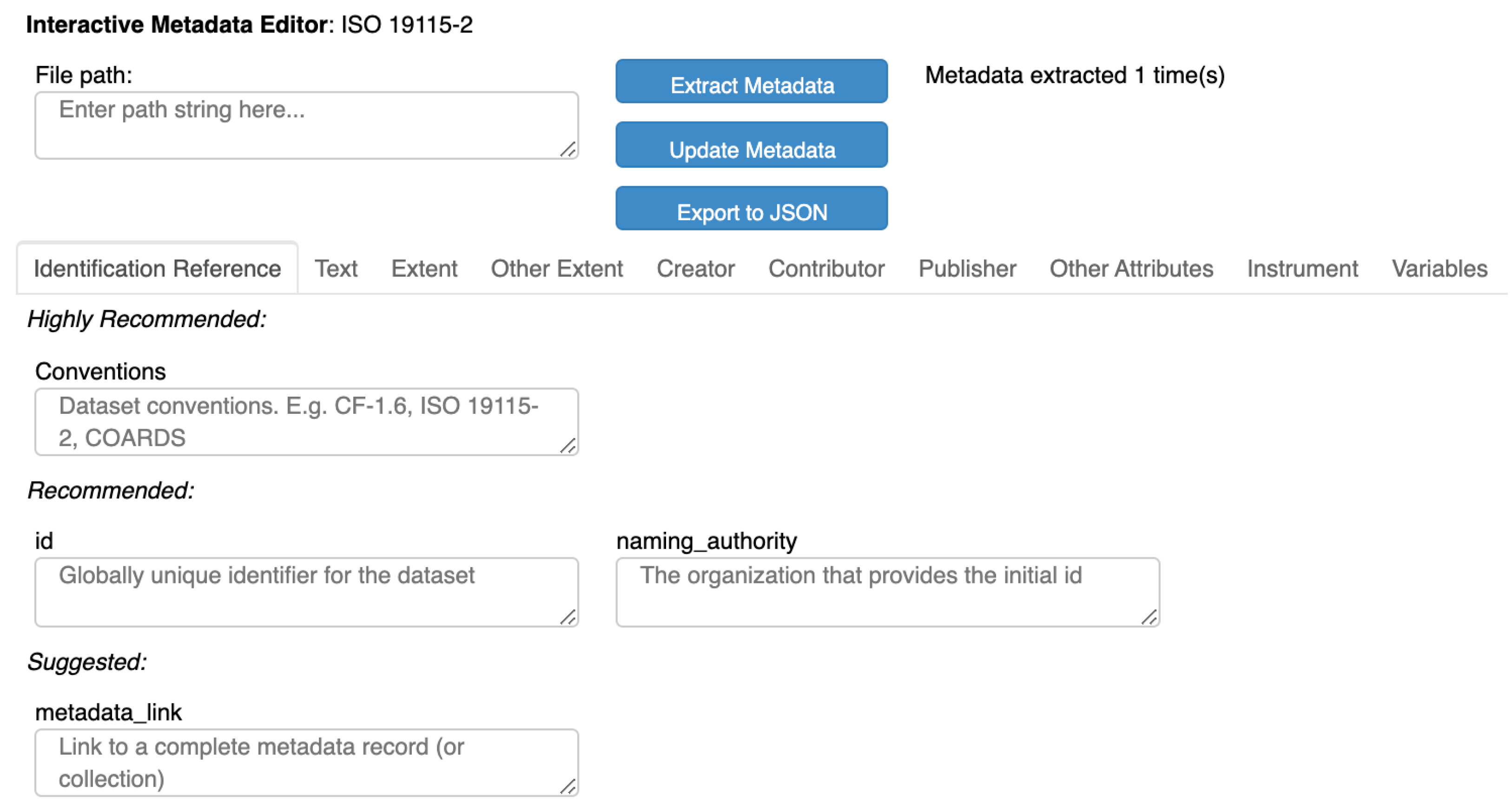
Our focus on documentation also extends to datasets in the form of metadata, an often underappreciated aspect of data collection.

Metadata

Built on the HDF5 format, we used the NetCDF format [26] to store each datacube in a standardised self-describing way that made it easy to access and share. Often, the metadata work is laborious and taken for granted, so, as part of pioneering a complete solution for creating hyperspectral datasets, openhsi includes an interactive ISO 19115-2:2019 metadata editor to record geographic and instrument information.

The widget shown in Figure 9 includes tabs for the various metadata sections and each text field includes a descriptive placeholder. A .nc file can be loaded, which will populate the existing fields and can subsequently be modified and updated in-place. Metadata can also be preconfigured to be included with each dataset when saved.

We take this ‘extra’ step of including a metadata editor because missing metadata can lead to misleading assumptions, and negatively impact downstream tasks by creating inaccurate models [27]. As suggested in [28], we believe that each dataset should be accompanied by a datasheet that documents its motivation, composition, collection process, and recommended uses. Having compliant metadata is necessary to create well-documented datasets. These features encourage a consistent basis for the communicating and sharing of hyperspectral datasets—which is currently lacking in the microscale HSI space.

5. Spectral Calibration, Optical Corrections, and Radiance Datacube

The next set of tasks for the software suite is to calibrate the imaged spectrum, perform the smile and flat-field optical corrections, and perform radiance conversion, as visualised in Figure 10. Rather than discussing this process abstractly, we will illustrate its use to obtain a reflectance datacube from raw data defined as digital numbers (DNs).

5.1. Spectral Calibration and Optical Corrections

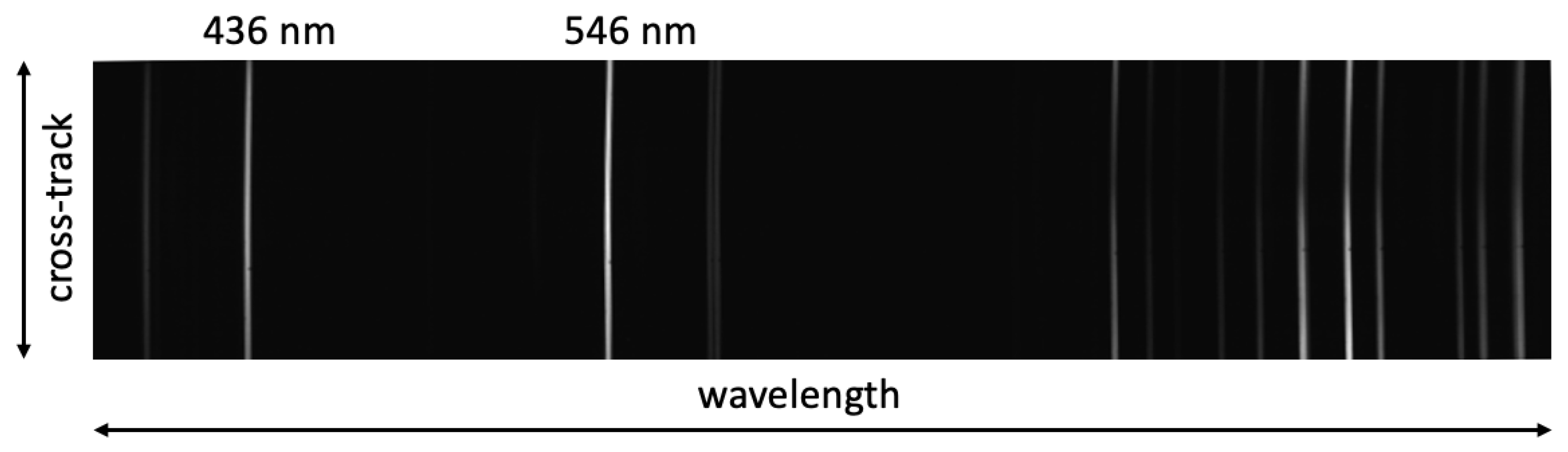
A HgAr source was used to evaluate how well OpenHSI can resolve emission lines and correct for smile artefacts. For a specific instrument, this calibration step may need to be redone occasionally due to optical degradation, aberrations, and misalignments from vibrations over time. We also found that adjusting the focus will shift the spectral range.

Figure 11 is an unprocessed frame captured by OpenHSI. The brightest emission lines at 436 nm and 546 nm are spectrally resolved. However, the slight curve near the top and bottom is indicative of smile error and needs to be corrected so that each column is associated with the same centre wavelength. It is important to reduce the tilt in the spectral lines by careful rotation of the slit in the lens tube.

To find the required wavelength shifts for each cross-track pixel, we apply a fast smile correction algorithm based on 1D convolution. Knowing that each cross-track pixel is similar to each other, a spectral row is used as the convolution window. Since the convolution equation will flip the window function, we simply provide the algorithm with a pre-flipped window. Using a predicted spectrum as the window function is also possible, as done in [29]. The peaks in the convolved outputs are then the smile correction offsets correct to the nearest pixel. Since applying this correction only requires changing the memory view of the array, this can be done quickly and in real time.

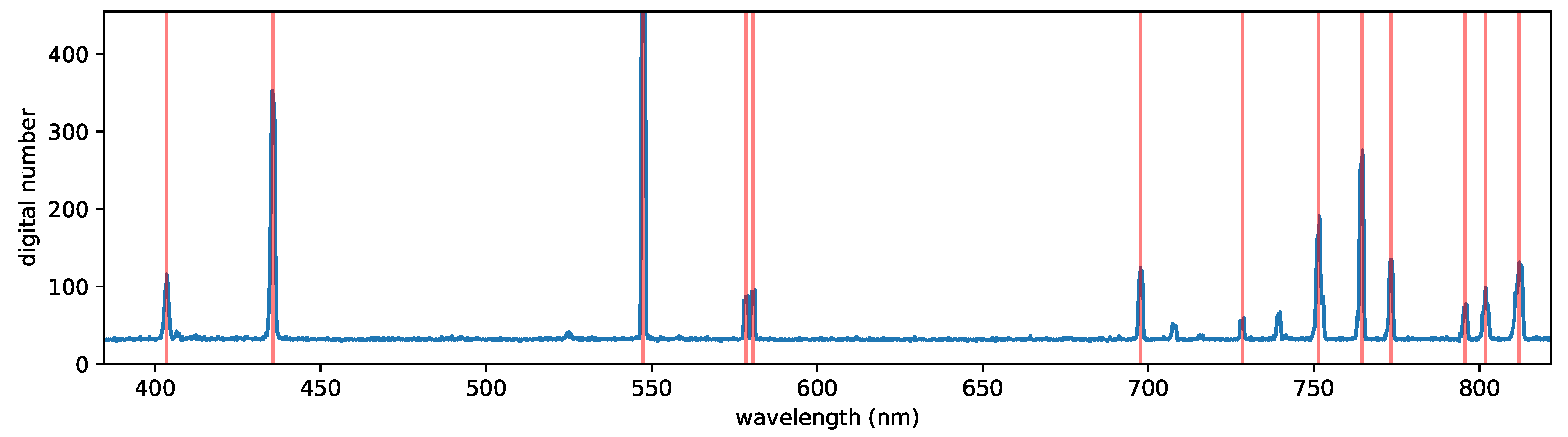
From the known emission lines, a peak finding algorithm is used along the centre cross-track pixel to find the column index of each detected peak. Assuming that each peak is Gaussian, a curve fit is applied to refine the centre wavelengths, as shown in Figure 12. The peak locations and known emission wavelengths are then interpolated to provide a column wavelength map. For the OpenHSI camera that we analysed, each column index corresponded to an ≈0.21 nm increment. The columns can then be binned down to a user-configurable full width at half maximum. Using a linear interpolation, the absolute error was ±3 nm, whereas a cubic interpolation gave an absolute error of ±0.3 nm. Using higher-order polynomials did not reduce the error because of overfitting.

Due to atmospheric scattering and absorption, which broaden fine spectral features, being able to resolve sub-nanometre features is unnecessary so, in our applications, we binned to 4 nm. This binning allowed us to achieve the SNR presented in Figure 5. Two methods for spectral binning are provided, depending on processing requirements.

For real-time processing, the fast binning procedure assumes that the wavelengths are linearly dependent on the column index because the binning algorithm consists of a single broadcasted summation with no additional memory allocation overhead. A slower but more accurate spectral binning procedure is also provided; it uses a cubic interpolation scheme to relate wavelength to column index but requires hundreds of temporary arrays to be allocated each time. In practice, slow binning is 2 ms slower than fast binning (which typically takes ≤0.4 ms). Binning can also be done in post-processing after collecting raw data.

When assembling the optics, a dust particle lodged in the slit and caused a cross-track artefact to appear in the form of a dark horizontal row. Furthermore, experiments imaging black and white bars showed insignificant keystone error, suggesting that the spatial pixels are spectrally pure. From this, we concluded that the keystone error was negligible (less than one pixel) and thus did not correct for it. Quantifying the keystone error would be a subject for future improvement.

Since not all pixels are illuminated on the sensor, we used a halogen lamp to determine the correct crop window.

All of these calibration steps are abstracted into a Python class DataCube built upon a custom circular array buffer implementation. After a data collect, the datacube can be saved in NetCDF format with named dimensions and metadata using the xarray package [30].

5.2. Radiance Conversion

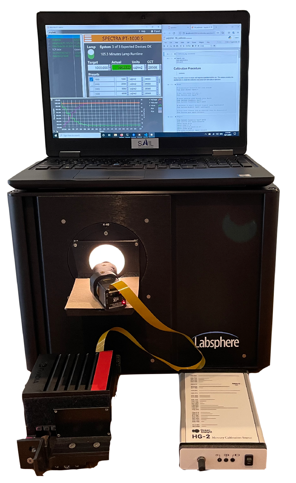
To ensure that artefacts due to pixel-level variations in sensitivity are removed, we convert from DNs to spectral radiance and calibrate using an integrating sphere. The setup used is shown in Figure 13.

To quantify the dark current, we recorded the raw camera DNs with the lens cover on in an unlit room for a variety of integration times and formed a look-up table. We also measured the DNs when the integrating sphere was set to a range of luminances.

The raw DNs can be converted to spectral radiance L by computing

$$L=\left(\mathrm{DNs}-{\mathrm{DNs}}_{\mathrm{dark}}\right)\times \left(\frac{L_{v,\mathrm{ref}}}{{\mathrm{DN}}_{L_{v,\mathrm{ref}}}}\right)\times \left(\frac{L_{\mathrm{reference}}}{53,880}\right).$$

(4)

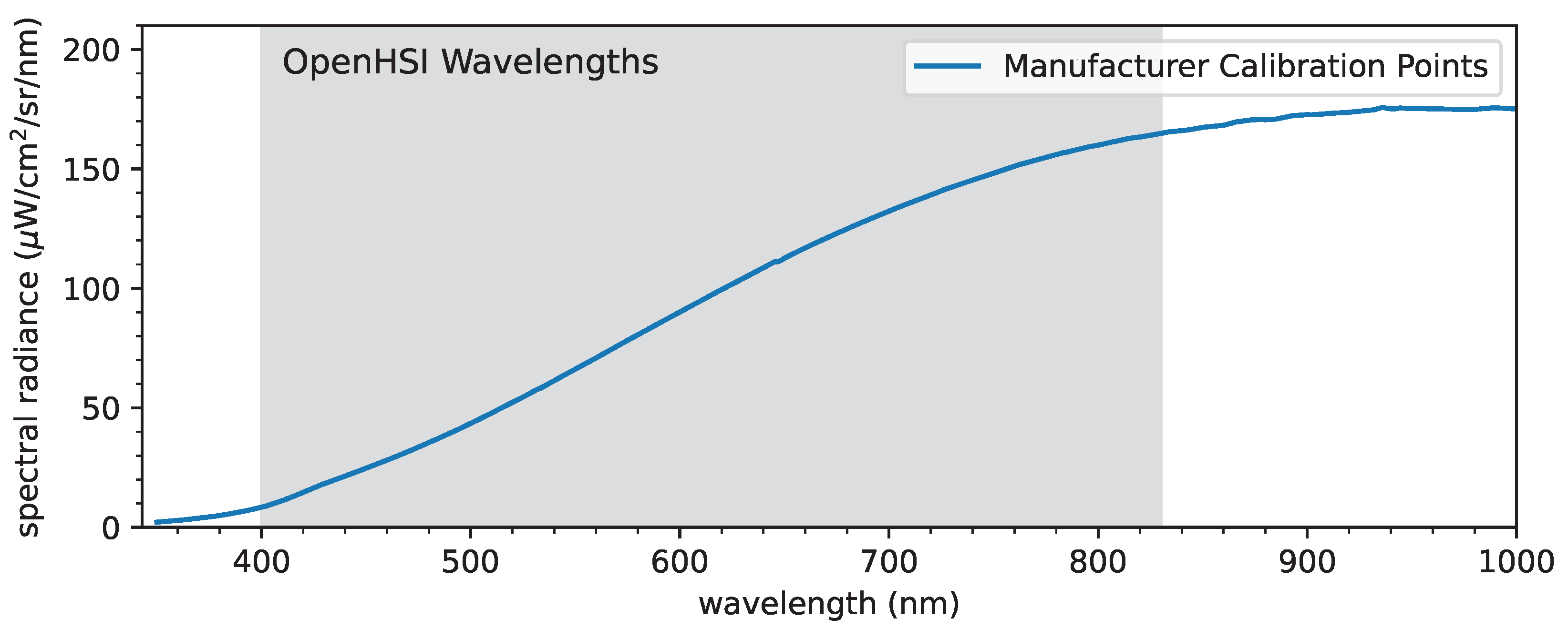
As each line is acquired, the dark current digital numbers DNs${}_{\mathrm{dark}}$ are subtracted and divided by the reference digital numbers at a given luminance DNs${}_{L_{v,\mathrm{ref}}}$ to obtain a dimensionless ratio. This is then multiplied by the corresponding luminance value $L_{v,\mathrm{ref}}$ to obtain pixels in units of luminance (Cd/m${}^2$). The manufacturer of the integrating sphere provides the spectral radiance $L_{\mathrm{reference}}$ when set to a luminance of 53,880 Cd/m${}^2$. We use this to convert the luminance pixels to spectral radiance by dividing by 53,880 Cd/m${}^2$ to obtain a dimensionless ratio and then multiplying by the manufacturer’s reference curve $L_{\mathrm{ref},53880}$ shown in Figure 14, which has units of spectral radiance (µW/cm${}^2$/sr/nm).

By converting to radiance, we were able to attenuate the effects of vignetting predicted from the Zemax simulation and also perform a flat field correction. We now proceed to calculate surface reflectances from the calibrated spectral radiance datacube using two approaches.

6. Radiometric Correction

Hyperspectral data acquired from airborne platforms are influenced by atmospheric absorption and scattering, as well as the sensor–target illumination geometry. In order to obtain nadir reflectance, radiometric correction is needed. The openhsi package includes two methods to achieve this based on (1) an open-source radiative transfer code written in Fortran called 6SV [31] with a Python wrapper Py6S [32] and (2) empirical line calibration (ELC).

6.1. Radiative Transfer Code (6SV)

A radiative transfer code models the interaction of sunlight as it enters the Earth’s atmosphere, reflects off the Earth’s surface, and travels back up through the atmosphere until it reaches a sensor. It includes the effects of energy loss from absorption, energy gain from emission, and energy redistribution from scattering [33].

To use 6SV, certain geographic information and local weather conditions need to be known: latitude, longitude, altitude, UTC time, zenith and azimuth angles, atmospheric profile, aerosol profile, and operating wavelengths. The default atmospheric profile used in openhsi is mid-latitude Summer and is augmented by local radiosonde data from the University of Wyoming (weather.uwyo.edu/upperair/sounding.html, accessed on 5 April 2022). If local pressure, temperature, and humidity is measured, these can be used to further parameterise the 6SV model.

We assumed that the ground reflectance is a homogenous Lambertian with a spectrally constant reflectance value of unity. This simulated the white reference that would normally be obtained using a spectralon panel in the lab. The 6SV reflectances can be calculated as the ratio of the measured radiance divided by the solar radiance at the sensor.

6.2. Empirical Line Calibration

If there are calibration targets with known spectral signatures in the data, we can also use ELC instead of 6SV to estimate a reflectance. ELC is a method to predict reflectance by solving a system of linear equations

$$L_i\left(\lambda \right)=\widehat{a}\left(\lambda \right){\rho }_i\left(\lambda \right)+\widehat{b}\left(\lambda \right)$$

(5)

that relate the at-sensor radiance L and reflectance $\rho$, where $\lambda$ is the wavelength, $\widehat{a}$ is the gain, and $\widehat{b}$ is the offset. This method requires ground truth data. We use calibration tarps but, in principle, tarps are not necessary as long as there are other objects in the scene with known spectra.

By using a dark and a bright target, the gain and offset estimated are suitable for the values in between. It takes some experimenting to check how ELC performs so openhsi provides an interactive tool. Users can draw and move bounding boxes which specify which pixels contribute to ELC. Equation (5) is shaped into the form $A\mathbf{x}=\mathbf{b}$, where

$$A=\left[\begin{array}{cc}{\rho }_1\left(\lambda \right)& 1\\ ⋮& ⋮\\ {\rho }_n\left(\lambda \right)& 1\end{array}\right],\mathbf{x}=\left[\begin{array}{c}\widehat{a}\left(\lambda \right)\\ \widehat{b}\left(\lambda \right)\end{array}\right],\mathrm{and}\mathbf{b}=\left[\begin{array}{c}{L}_1\left(\lambda \right)\\ ⋮\\ L_n\left(\lambda \right)\end{array}\right].$$

(6)

To compute $\widehat{a}$ and $\widehat{b}$ for all spectral bands efficiently, we stack many matrices together to form a rank three tensor that can be solved in one pass. When the system of equations is overdetermined, openhsi will use the pseudo-inverse $\mathbf{x}={\left(A^{T}A\right)}^{-1}{A}^T\mathbf{b}$ to find a least squares solution.

Once $\widehat{a}$ and $\widehat{b}$ are known, the estimated reflectance $\widehat{\rho }$ can be computed using

$$\widehat{\rho }\left(\lambda \right)=\frac{L\left(\lambda \right)-\widehat{b}\left(\lambda \right)}{\widehat{a}\left(\lambda \right)}.$$

(7)

7. Performance

The OpenHSI camera and software were flown on a Matrice 600 drone over a coastal land–beach–ocean region near Cairns in Queensland, Australia, on May 26th. A Ronin gimbal minimised distortion during flight and allowed the camera to be pointed at nadir from 120 m above the surface. At this height, the swath width was 22.6 m and the ground sample distance was 5 cm. Using an exposure time of 10 ms, the OpenHSI camera was able to run at 75 FPS so a flight speed of 3.8 m/s was chosen to achieve square pixels. We flew at around 2 pm local time when it was low tide.

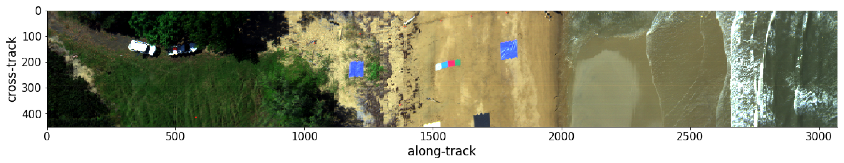
Within the scene imaged, we placed several calibration tarps of various colours labelled in Figure 15 (an RGB visualisation using the 640, 550, and 470 nm bands after smile correction and binning). The colour scale for the digital numbers is set by the 2–98% percentile to prevent outlier pixels from reducing contrast. openhsi also offers a histogram equalisation option as another robust visualisation option. Without the robust option, the specular reflection from the waves and the car roofs means that the rest of the scene appears dark and features are difficult to distinguish. The 293rd cross-track pixel appeared as a dark horizontal stripe through the whole scene; this was due to a dust particle on the imaging slit that resisted cleaning efforts.

After converting to radiance, the same scene is shown in Figure 16 using the same bands and robust visualisation option. The dark horizontal stripe from Figure 15 is now almost eliminated. From visual inspection, the colour representation is faithful to the eye observations and weather conditions on site.

To validate the spectral performance of the OpenHSI imaging spectrometer, we converted the radiance measured for the calibration tarps to reflectance and compared it to lab-based reflectance readings using an ASD Fieldspec 4 spectrometer.

7.1. Calibration Tarps

The tarps listed in

Table 3. Calibration tarp information.

Tarp Name	Information
gray	Type822 3 m 48% October 2016 Group VIII Technology
charcoal	Type822 3 m 6.5% October 2016 Group VIII Technology
cyan, magenta, green	Type822 1.2 × 3.6 m C/M/G March 2017 MFG Group VIII Technology
blue	Water and UV resistant high-density polyethylene weave

are designed to have a flat spectral signature at the given reflectance percentage. We also include coloured tarps to verify the spectral performance after calibrating using the gray tarps.

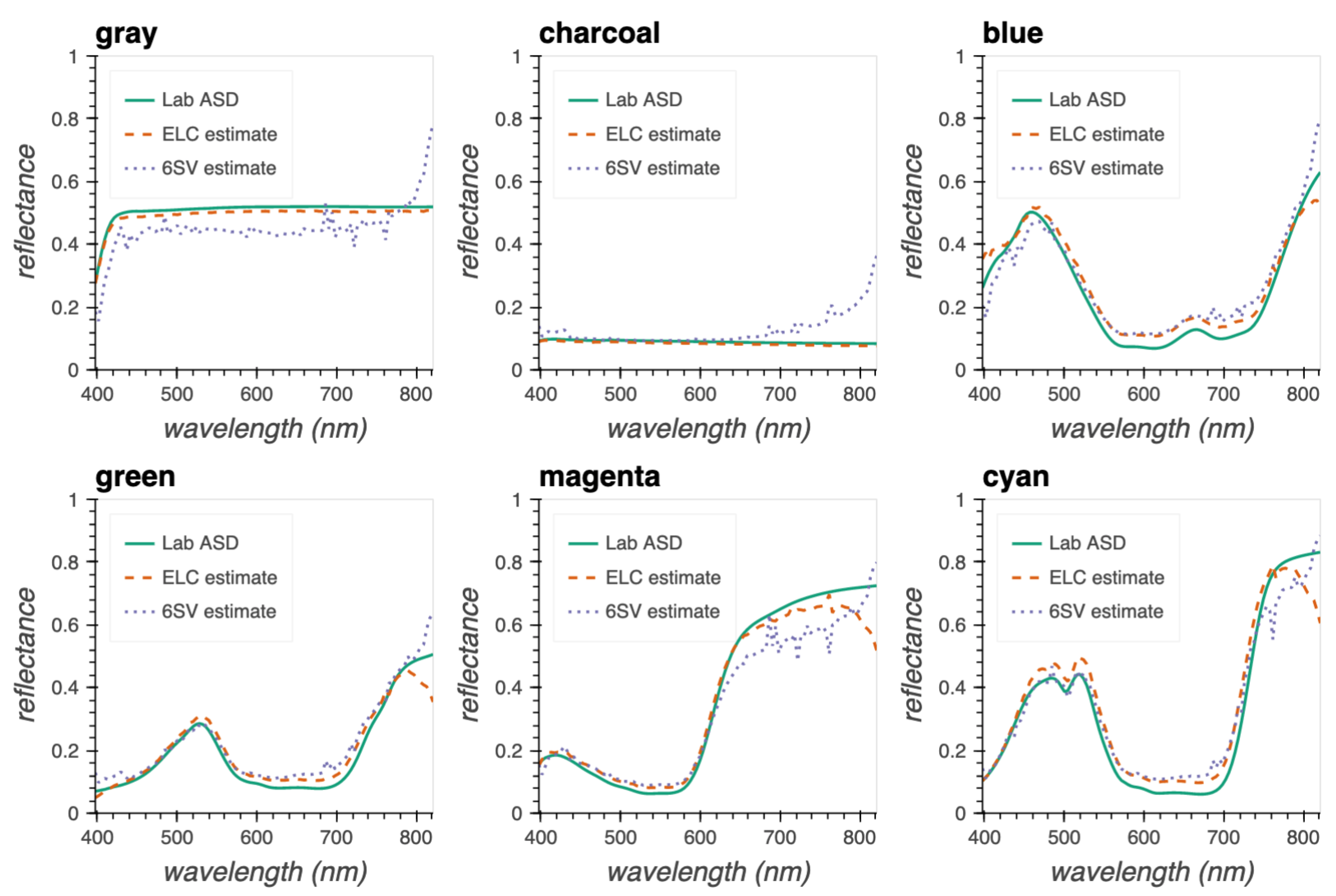
Since the ASD Fieldspec 4 measured reflectance from 350 to 2500 nm in 1 nm increments, we interpolated these to match the OpenHSI wavelengths and then compared with the reflectances estimated using both 6SV and ELC. Using the interactive ELC tool referenced in Section 6.2, pixels on the gray and charcoal tarp were used in the ELC algorithm. For the 6SV model, the nearest radiosonde data at Willis Island were used in the atmospheric profile to compute the radiance at the sensor. The results are compared in Figure 17.

For each tarp, we averaged the selected middle region away from the boundary to reduce any adjacency effects from other tarps and sand. This was not possible for the gray and charcoal tarps since most of the tarp was clipped. Due to strong wind, the blue tarp closest to the water showed ripples, so we used the blue tarp on the left instead.

The ELC estimates for the gray and charcoal tarps matched the ground truth, which was expected because they were used as the ELC reference. For the other tarps, the ELC estimates agreed quite well with the ASD reflectances, with relatively minor differences in magnitude. It consistently underestimated the infrared > 780 nm. We believe that this is because most of the gray tarp was clipped and the reference pixels chosen had a component of sand that was blown on top. Using other calibration tarps in the ELC algorithm could, in principle, fine tune the ELC estimates for the rest of the dataset and reduce the impact of the clipped gray tarp. When this was done, the dip in the infrared was reduced but still present.

Typically, the 6SV results follow the ASD and ELC results quite well in magnitude and large-scale trends for the charcoal, blue, green, magenta, and cyan tarps, but less well for the grey tarp. However, artefacts from atmospheric absorption bands are apparent in all the tarps for the 6SV results above approximately 700 nm—in particular, the O${}_2$-A absorption line at 760 nm. During our time on site, the cloud cover varied rapidly so the radiosonde data from the nearest weather station four hours earlier may not be an accurate representation of H${}_2$O content in the atmosphere. Furthermore, the 6SV results for all the tarps show a sharp rise at >800 nm and this is most apparent in the charcoal tarp. We hypothesise that this is due to some order overlap from the transmission grating that we used, leading the camera to measure more signal in that spectral region than what is predicted using 6SV. Our experiments with building and calibrating these hyperspectral imaging spectrometers using other cameras indicate that this order overlap does occur. Generally, the 6SV calculations tend to overestimate the atmospheric absorption but are still accurate enough to identify calibration tarps interactively in our ELC explorer widget.

7.2. Future Work

While the OpenHSI camera was stabilised with the Ronin gimble, some oscillations persisted and this was apparent from the warped edges of the vehicles and the tarps. To remove this warping, georectification is needed to locate each pixel to a coordinate system. This also facilitates the stitching of multiple swaths into a single dataset so that the full gray tarp can be recovered despite being clipped. Moreover, to improve the 6SV results produced via Py6S, we plan to collect pressure, humidity, and temperature data during future trials and validate whether the local radiosonde data are suitable. Furthermore, to deal with diffraction order overlap, we plan to include an order sorting filter or long-pass filter to choose where order overlap occurs.

To increase the number of photons incident on the detector and thus increase the SNR at the cost of some spectral resolution, a wider slit can be used. This would allow the camera to use a lower exposure while still retaining sufficient signal, operate at a higher frame rate, and be flown at a faster speed. Furthermore, due to the design and choice of components and detector, OpenHSI is only capable of imaging the visible–NIR spectrum, which limits the scope of what can be studied. To address this, one could operate another OpenHSI designed for the shortwave infrared range of 1–2.5 $\mathsf{\mu }$m in tandem and co-register the pixels.

For a first application of a microscale HSI built from COTS components with calibration and radiometric correction presented in this paper, these results illustrate the great promise that OpenHSI has for real-time data collection and analysis. An exciting development is that a variant of the OpenHSI camera will be used in the RobotX 2022 competition (http://robotx.org/programs/robotx-challenge-2022/, accessed on 5 April 2022), a nexus for many other research applications beyond imaging coastal regions, as presented in this work.

8. Conclusions

The central motivation of OpenHSI was to improve HSI accessibility and the acquisition, calibration, and analysis of hyperspectral datasets through open-source designs and software. We successfully demonstrated a compact and lightweight pushbroom hyperspectral imaging spectrometer made from COTS components. The key improvement upon the HSI introduced by [21] is a more uniform focus across the spectral range, which translates to better spatial contrast for spectral bands. An extensive software package, openhsi, was developed and optimised to simplify the process of capturing calibrated and corrected hyperspectral datacubes on development compute platforms.

To increase the adoption of microscale hyperspectral imaging spectrometers, we focused on software documentation from the outset via a literate programming approach. The end result is a holistic package that allows practitioners to interactively visualise, process, and create documented datasets with ISO 19115-2 metadata. We evaluated our smile correction, spectral binning, radiance conversion, and radiometeric correction routines (using 6SV and ELC) and optimised them for real-time processing. Finally, we flew the OpenHSI camera and software on a drone and verified the spectra collected using calibration tarps. It is our hope that OpenHSI will be the first step of many to removing barriers to the widespread use of hyperspectral technology.