Article

Precipitation Microphysics of Tropical Cyclones over Northeast China in 2020

1
Key Laboratory of Tropical Atmosphere-Ocean System, Ministry of Education, School of Atmospheric Sciences, Sun Yat-Sen University, Zhuhai 519000, China
2
Southern Marine Science and Engineering Guangdong Laboratory (Zhuhai), Zhuhai 519000, China
3
Opening Key Laboratory for Northeast Cold Vortex Research, Institute of Atmospheric Environment, China Meteorological Administration, Shenyang 110166, China
4
Shenzhen National Climate Observatory, Shenzhen 518040, China
*
Author to whom correspondence should be addressed.
Remote Sens. 2022, 14(9), 2188; https://doi.org/10.3390/rs14092188
Submission received: 7 April 2022 / Revised: 1 May 2022 / Accepted: 2 May 2022 / Published: 3 May 2022

Abstract

:
Landfalling tropical cyclones (TCs) in Northeast China are rare because of the region’s high latitude (>40°N). In 2020, Northeast China was affected by three TCs within half a month—the first time on record. We used the Global Precipitation Measurement orbital dataset to study the precipitation microphysics during the TC period in Northeast China in 2020 (2020-TC), and during September in this region from 2014 to 2019 (hereafter September 2014–September 2019). FY-4A was used to provide cloud top height (CTH). The results show that, compared with September 2014–September 2019, the 2020-TC precipitation has stronger precipitation ice productivity, weaker deposition efficiency, stronger riming, and stronger coalescence processes. The storm top height (STH), CTH, and the difference between the two (CTH-STH) are indicative of the near-surface droplet size distribution (DSD), but there are differences: STH and CTH-STH both correlate significantly with mean mass-weighted drop diameter, whereas only the positive correlation between CTH and normalized drop concentration parameter passes the significance test. These results reveal for the first time the precipitation microphysics of landfalling TCs in Northeast China, and allow discussion of the validity of convective intensity indicators from the perspective of DSD.

1. Introduction

Landfalling tropical cyclones (TCs) usually bring strong winds and heavy precipitation, which may cause serious economic losses and even endanger human life. Improving the quantitative precipitation estimation of landfalling TCs depends on an accurate understanding of microphysical processes, because the microphysics of TC precipitation and local precipitation are significantly different [1,2,3,4]. Droplet size distribution (DSD) is the basic parameter of precipitation microphysics, and there have been many studies on the DSD of TC precipitation and its corresponding microphysical processes. It is generally believed that landfalling TC precipitation has a high raindrop concentration and small raindrop diameter, and that the warm rain processes (accretion and coalescence) are dominant [5,6,7,8].
Located in the western North Pacific, China is one of the countries most threatened by TCs. Funded since 2009, the national Landfalling Tropical Cyclone Research Project (LTCRP) in China has built a large number of ground-based observation systems in East China and South China [9]. For example, a study using polarimetric radar found that landfalling TCs in South China have a larger raindrop diameter and lower raindrop concentration than those in East China [6,8]. However, LTCRP has not established observations in Northeast China (north of 40°N), because the number of TCs moving northwards is inherently small, and the energy of TCs in such a northerly location basically becomes exhausted. On rare occasions, however, the extratropical transition of TCs will bring TC-like conditions in summer and autumn to latitudes where such events would not normally occur, causing precipitation of a different nature to the usual local weather systems [10]. Wang et al. (2021) studied TC Yagi (201814), which converted to an extratropical cyclone, and found that its raindrop diameter was very different from normally observed landfalling TCs; specifically, it no longer possessed the characteristics of marine precipitation and instead was more typical of continental precipitation [11]. However, the instruments used in their research were actually located in East China (37°N, 117°E). At present, there is almost no research on the DSD and microphysical processes of landfalling TCs in Northeast China, which poses a significant challenge for local forecasters.
Fortunately, the rapid development of satellite remote sensing technology has provided us with an excellent opportunity to study the DSD and microphysical processes of landfalling TC precipitation in these areas lacking ground-based observations. The Global Precipitation Measurement (GPM) core satellite—the successor to the Tropical Rainfall Measuring Mission (TRMM)—was launched in February 2014. Different from the TRMM precipitation radar, the dual-frequency precipitation radar (DPR) the GPM carries can retrieve the three-dimensional DSD of precipitation [12]. There have been some studies on TCs using GPM DPR [13,14,15,16]. For example, Huang et al. (2022) found a good consistency of reflectivity between GPM DPR and ground-based S-band polarimetric radar on TC observation over South China, whereas underestimation was found for the raindrop number concentration [16]. However, there is a lack of polarimetric radar observations in Northeast China, and it is necessary for us to use satellite remote sensing with respect to the microphysics of mid-latitude TCs.
Storm top height (STH) and cloud top height (CTH) are widely used to characterize the convection intensity. STH, also known as echo-top height, indicates the maximum height a precipitation particle can reach. Stronger convection, capable of transporting larger particles and hydrometeors to higher altitudes and resulting in more latent heat release, may further exacerbate updrafts [17]. CTH is the maximum height of the visible part of the cloud, and is also the upper bound of the height of the condensation/nucleation of water vapor into cloud particles [18,19,20]. For example, Sun et al. (2021) used the Himawari-8 satellite to identify the overshooting tops of TCs and found that the overshooting tops of strong TCs and rapidly intensifying TCs are denser than those of weak TCs, as well as those of TCs that intensify or weaken slowly [21]. There have also been studies conducted suggesting that more comprehensive results can be achieved using CTH and STH together. Masunaga et al. divided precipitation into four categories: shallow convection has an STH of ~2 km, with an infrared brightness temperature of ~280 K, and warm rain processes dominate; cumulus congestus has an STH near the melting level, and the CTH does not reach the tropopause; deep stratiform has an STH near the melting level, but with very cold cloud tops; and deep convective has cloud tops as cold as deep stratiform, but the precipitation ice is more productive, forming at heights well above the melting level, thus with a higher STH [22,23,24]. Therefore, Liu et al. (2007) pointed out that the difference between the CTH and STH (CTH-STH) can be considered as another proxy for convection intensity—a smaller difference indicates a stronger convective core that lifts large particles closer to the cloud top [25].
STH, CTH, and CTH-STH are closely related to the near-surface DSD. Deeper systems can provide an environment that favors the production of larger raindrops through the process of collision–coalescence [1,14]. For example, Smalley and Rapp (2021) showed that in shallow cumulus clouds, keeping the humidity constant, the ratio of the cloud water path to rainwater nearly doubles for every 0.5 km increase in CTH for a given range [26]. The rain rate below the melting level increases with the STH until the STH reaches 8–9 km [27]. Deeper systems can also increase ice-phase processes, producing larger snowflakes or graupel—before the rapid intensification of TCs, there is the strongest increase in hydrometeor mass upward flux at the height of 10–15 km [28]. One of our group’s previous studies shows that as the STH grows from 4 km to 10 km, the near-surface raindrop diameter increases from 1.0 mm to 1.5 mm, mainly due to the process of riming and aggregation [29]. When CTH-STH is smaller (greater), it indicates a greater (smaller) ratio of hail/graupel particles to snow, and this structure cannot currently be captured by cloud-resolving models [30].
Within half a month from 27 August 2020, Northeast China was successively struck by three TCs (Bavi (202008), Maysak (202009), and Haishen (202010)), for the first time on record. The lowest pressures of the three TCs were 950 hPa, 935 hPa, and 910 hPa, respectively. Since the meridional circulation composed of the subtropical high and cold vortex remained relatively stable during this period, all three TCs were guided to move northward along a “straight” path (Figure 1). As the latitude of the TCs continued to increase, the thermal conditions on the sea surface deteriorated, the dry and cold air in the north gradually strengthened, and the TC intensity gradually weakened. The three TCs made landfall with 10-min maximum sustained winds at 35 m s−1, 42 m s−1, and 40 m s−1, respectively. However, after these TCs entered the mid-latitudes, they combined with cold air and transformed into extratropical cyclones, which affected a wider area and brought stronger rainfall and local instantaneous high winds. The daily rainfall recorded at 49 national-level observation stations in the provinces of Jilin and Heilongjiang exceeded the historical extreme value in September, and the rainfall in some areas was more than four times that of the same period in normal years.
This paper focuses on the microphysical characteristics of TC precipitation in Northeast China and its relationship with the STH and CTH. Since this area is generally rarely affected by TCs, the public and government have not paid enough attention to them, and forecasters also lack the necessary physical understanding of TC precipitation. We therefore hope that this study can address these issues by reporting and discussing microphysical observations of landfalling TC precipitation in Northeast China.

2. Data and Methods

We used DPR_NS (Ku normal scan) data from GPM 2ADPR in September 2014–September 2020. These data provide vertical profiles of DSD and radar reflectivity with a vertical interval of 125 m and a horizontal resolution of 5 km. DSD consists of the normalized drop concentration parameter (dBNw) and mean mass-weighted drop diameter (Dm), retrieved by the dual-frequency method at the Ku inner swath and by the single-frequency method at the outer swath. The units of Nw and Dm are mm−1 m−3 and mm, respectively. DSD has been shown to be in good agreement with ground-based observations in limited local areas all over the world [32,33,34,35]. The minimum radar detection threshold for KuPR is 15.5 dBZ [36].
The study area (Northeast China) is (40°–53°N, 115°–135°E) (Figure 2), and the statistics in the Results section are all based on GPM DPR pixels. The warm season in this area spans from May to September every year. The cold vortex is the dominant weather system in this region during the warm season, contributing ~50% of total precipitation [37]. Considering the large-scale precipitation in the study area affected by the cold vortex around 31 August 2020, it is difficult for us to distinguish whether this precipitation should be attributed to the cold vortex or the dissipated TC Bavi. Therefore, we selected GPM 2ADPR data from 2 to 9 September 2020. The precipitation in this area during this period can be considered to be entirely caused by TC movement and dissipation (hereafter referred to as 2020-TC). We used the GPM 2ADPR data of the region in September from 2014 to 2019 for comparison (hereafter referred to as September 2014–September 2019).
CTH retrieved by the FY-4A Advanced Geostationary Radiation Imager (AGRI) was used in this study. FY-4A is a new-generation Chinese geostationary satellite. The AGRI instrument on board performs a full-disk scan every 15 min and measures 14 spectral channels ranging from 0.47 to 13.5 μm [38]. The AGRI cloud product algorithm partly inherits the FY-2 algorithm, and partly refers to the GOES-R algorithm [39]. Briefly, retrieval of cloud top pressure mainly relies on two IR window bands (11 and 12 µm) and a single CO2 absorption band (13.5 µm), and then CTH is calculated using the Numerical Weather Prediction temperature profiles with a horizontal resolution of 4 km. This product has been widely used in cloud and precipitation research [40]. Compared with the Moderate Resolution Imaging Spectroradiometer (MODIS), AGRI underestimates the CTH by 1.366 ± 2.235 km over the Tibetan Plateau, a region with complex topography [41].
Because the study area is located in the mid-latitudes, where the observation capability of the geostationary satellite is weaker than that in the low latitudes, it is first necessary to test the reliability of the FY-4A CTH in this area. Cloud product data (MOD06L2 and MYD06L2) derived from MODIS were used for comparison. MODIS provides cloud top height at a resolution of 1 km × 1 km. Figure 2 shows an example of the quasi-simultaneous observations of MODIS, FY-4A, and Himawari-8 on 8 September 2020 at 05:15, 05:15, and 05:10 UTC, respectively. At this time, TC Haishen had transformed into an extratropical cyclone, but it affected almost the entire study area. The cloud displayed by the three products are similar in shape, all rotating in a cyclonic shape. The maximum CTH observed by MODIS reaches up to 14 km, mainly distributed to the northwest and south of the TC center. The CTHs of FY-4A and Himawari-8 also reach a maximum in this area, but the maximum CTH is less than 12 km. Between the spiral cloud belts and beyond the TC cloud belt, there are many low clouds, and the CTH retrieved by MODIS is lower. The CTHs of FY-4A and Himawari-8 are similar in value, but the CTH of FY-4A looks smoother, and Himawari-8 shows more detail, which may be related to their different sensitivity.
To quantitatively demonstrate the reliability of the FY-4A CTH, we performed a pixel-to-pixel comparison using all CTH observations from 2 to 9 September 2020. Only both “cloudy” pixels were involved in comparison. We used the CTH of Terra and Aqua MODIS to compare with the FY-4A CTH, which guaranteed an adequate contrast between day and night. Specifically, the FY-4A observation closest to the MODIS observation time was selected, and the MODIS pixels with a distance of less than 4 km from the FY-4A pixel were arithmetically averaged to obtain the FY-4A and MODIS pixel-to-pixel CTH comparison. The results are shown in Figure 3a, from which we can see that the CTH has two large values of occurrence frequency at ~2 km and ~10 km. The FY-4A CTH is generally higher than the MODIS CTH at ~2 km, and the FY-4A CTH is lower at ~10 km. Overall, FY-4A underestimates the CTH by 1.12 ± 2.49 km compared with MODIS, and this error is slightly lower than the results of reference [41] over the Tibetan Plateau, which may be because the topography of Northeast China is less complex than the Tibetan Plateau. The inconsistency between the two is mainly due to the difference in CO2 absorption bands—FY-4A AGRI has one, and MODIS has four.
The Himawari-8 CTH was also used for a quantitative comparison with the FY-4A CTH. Since the Himawari-8 official product only uses daytime observation data to retrieve CTH, we also only used the daytime FY-4A CTH for the comparison. Himawari-8 provides 0.05° gridded CTHs, and the closest FY-4A pixel to the Himawari-8 grid was used for comparison with Himawari-8. As shown in Figure 3b, the CTHs of Himawari-8 and FY-4A are consistent, and the FY-4A CTH is lower by 0.21 ± 2.40 km, which may be due to their similar retrieval channels.
The above comparison shows that it is reasonable to use the FY-4A CTH during the 2020-TC period. When matching the pixels between GPM DPR and FY-4A AGRI, the DPR pixel was used as the benchmark, and the nearest FY-4A pixel was selected to provide the CTH of the DPR pixel.

3. Results

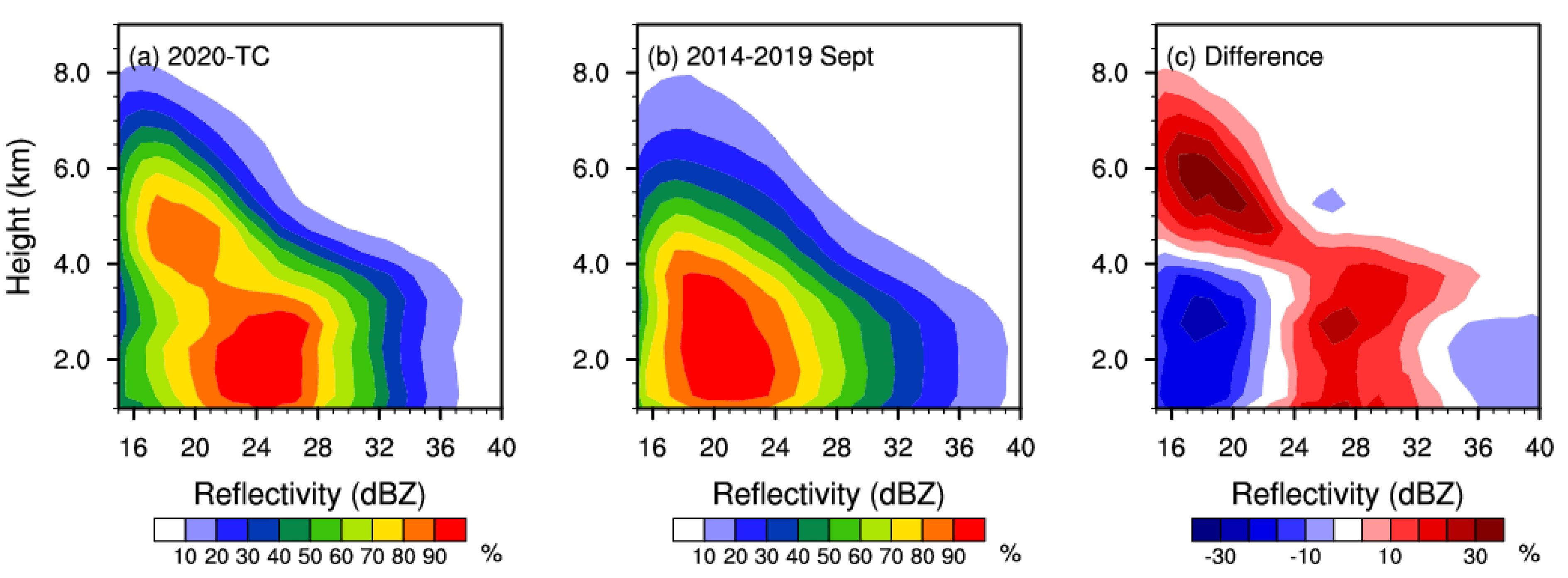
3.1. Differences in Precipitation Microphysics between 2020-TC and September 2014–September 2019

Figure 4 shows the reflectivity CFADs (contoured frequency by altitude diagrams) of the 2020-TC period, September 2014–September 2019, and their difference over Northeast China. Total number of DPR profiles is 36,661 and 240,781, respectively. The reflectivity was interpolated into bins with a vertical interval of 0.5 km and a horizontal interval of 1 dBZ. A minimum threshold of 100 in each bin was used to avoid noise. Values were normalized with the overall maximum, which ensured that the value in each bin was between 0% and 100%, where 100% is equivalent to 9694 observations in (a) and 60,973 observations in (b). The difference in CFAD was directly obtained by subtracting the 2014–2019 CFAD from the 2020-TC CFAD. As pointed out by Zagrodnik et al. (2019), compared to layer-by-layer normalization, normalizing by overall maximum allows the differences between different heights to be compared [42].
During the 2020-TC period, at altitudes above 5 km, the reflectivity exhibits a constant slope—the 50% contour increases from 17 dBZ at 6.75 km to 24 dBZ at 5 km (growth rate of 4 dBZ km−1). In contrast, the 50% contour for September 2014–September 2019 does not reach the height of 6.5 km, but it increases almost linearly from 18 dBZ at 5.75 km to 23 dBZ at 5 km (growth rate of 6.7 dBZ km−1). This indicates that the precipitation during the 2020-TC period had a weaker deposition efficiency. Around 5 km, the CFAD of 2020-TC exhibits a distinct “shoulder”—the slope of reflectivity increases with decreasing altitude changes. The most obvious phenomenon is at the height of 5 km (28 dBZ) of the 10% contour. Above this height, the reflectivity increases slowly with the decrease in height—that is, the growth of ice-phase deposition only. Below this height, the rate of increase in reflectivity is almost twice as fast as before, which is indicative of the contribution of mixed-phase riming. Correspondingly, the precipitation of September 2014–September 2019 does not show a rapid increase in reflectivity. Likewise, in the 2020-TC modal contours (e.g., the 70% contour), this phenomenon of mixed-phase growth becomes less pronounced, indicating that the riming process only existed in part of the precipitation in 2020-TC. At altitudes below ~3.5 km, the reflectivity of 2020-TC remains unchanged, indicating the presence of a melting layer and a near-equilibrium liquid-phase process. In September 2014–September 2019, the melting level is located at ~3 km. This suggests that the arrival of the TCs had raised the height of the melting level, providing sufficient vapor transport and development space for warm rain processes (collision–coalescence) [43].
From the difference in CFAD (Figure 4c), there is an obvious positive difference in the low reflectivity region of the ice phase (center at ~18 dBZ, 6 km). On the one hand, this is due to the difference in deposition efficiency mentioned earlier, while on the other hand, it is due to the stronger precipitation ice productivity of TCs [24]. This phenomenon can also be seen in Figure 4a,b—with a fixed reflectivity of 17 dBZ, the contours of 2020-TC are denser than those of September 2014–September 2019. Specifically, the maximum heights of the 10% contours of both are around 8 km, while the 2020-TC (September 2014–September 2019) 50% contour appears at 6.5 km (5.25 km). In the liquid phase, there is a strong negative difference at 15–20 dBZ, a moderate positive difference at 24–32 dBZ, and a weak negative difference at 36–40 dBZ. This indicates that there was more moderate precipitation rather than heavy precipitation in the 2020-TC period.
Figure 5 shows the joint probability distribution functions (PDFs) of the near-surface DSD. Compared with September 2014–September 2019, the precipitation during the 2020-TC period shows higher dBNw (36–50) with small Dm (0.8–1.6 mm), and moderate dBNw (32–36) with moderate Dm (1.2–1.6 mm). Correspondingly, although the near-surface Dm during September 2014–September 2019 is larger, it has a lower dBNw (<30), which would have made it difficult for a greater rain rate to generate [44,45]. The average dBNw and Dm are 34.4 (33.0) and 1.23 (1.28) mm for 2020-TC (September 2014–September 2019), respectively. Compared with the “maritime-like” cluster (dashed line box in Figure 5) and “continental-like” cluster (solid line box in Figure 5) proposed by Bringi et al. (2003) [46], both DSDs during 2020-TC and September 2014–September 2019 are significantly different from them, showing a smaller Dm. The DSD in Northeast China is more distributed near the fitting line of stratiform precipitation (dashed line in Figure 5). Meanwhile, comparing with specific observed events, the dBNw and Dm for TC landfall in Taiwan are 38 and 2 mm [1], and for TC landfall in East China, they are 46.7 and 1.41 mm [6], while for TC precipitation over the South China Sea, they are 44.7 and 1.49 mm [8]. These results are all larger than the landfalling TC precipitation in the present study, which indicates that the microphysics of landfalling TCs in Northeast China is very different from that in the tropics and subtropics. As reported in reference [43], landfalling extratropical cyclones over the west coast of North America have the most frequent drop size regime at dBNw values from 34 to 40 and Dm values from 1.0 to 1.6 mm. These are relatively close to our results, indicating that TCs in Northeast China possess the DSD characteristics of extratropical cyclones. However, it should be noted that these studies did not use the same method and instrument to retrieve dBNw and Dm, which may have caused some differences in values. Nonetheless, we believe that the retrieval accuracy of GPM DPR itself will not produce too much error, and therefore, the absolute errors of 2020-TC and September 2014–September 2019 would not be altered.
Figure 6 shows the vertical profile of the DSD for the two periods. Overall, dBNw during the 2020-TC period is 1 larger than that during September 2014–September 2019 (Figure 6a), which would have provided an excellent environment for particle collection. At the height of 6 km in the ice-phase region, the Dm of 2020-TC is less than 1.1 mm, while that of September 2014–September 2019 is greater than 1.2 mm (Figure 6b). This is because, on the one hand, with the strong updrafts of the TCs, more small particles would have been transported from the low level to the middle level, which would have reduced the particle size in the middle level; on the other hand, small particles compete with each other for water vapor in the process of nucleation and deposition, meaning each particle cannot grow rapidly. This phenomenon is also reflected in the CFAD—although greater dBNw exists in the ice-phase region of the 2020-TC precipitation, the reflectivity is proportional to the sixth power of the particle size, so there is a lower rate of increase in reflectivity in the ice-phase region in 2020-TC (Figure 4a). The height of 3–5 km is the main area in which mixed-phase processes occur. Affected by the updraft in the TC, riming occurs, and the particle size grows rapidly (increasing from ~1.13 mm to ~1.24 mm) as the ice particles from the upper layer fall and the droplets from the lower layer rise [47]. Correspondingly, although this process also exists in the precipitation of September 2014–September 2019, the Dm only increases by ~0.05 mm. This shows that mixed-phase processes were stronger during the 2020-TC period. Below 3 km is the liquid-phase region, and the Dm of both shows almost no change, indicating that the microphysical processes had reached an equilibrium as a whole.
By sorting the STH and averaging the samples, we calculated the relationship between the STH and near-surface DSD (Figure 7). Each point represents 10% of the sample size, bars correspond to the standard deviation of the DSD of those 10% samples, and the dashed line is the line of best fit. Figure 7a,b shows that there is a weak positive correlation between STH and dBNw, but neither one passes the 95% significance test. A clearly anomalous point is the lowest 10% STH, which corresponds to a large dBNw (~35.6 for 2020-TC, ~33.3 for September 2014–September 2019). These precipitation events are shallow convection, and warm rain processes dominate the mechanism for the generation of such precipitation [14,23]. The arrival of the TCs brought a large amount of water vapor to the low level, but limited by the development range of this type of precipitation (less than 3 km), the particles could not develop to a large extent. Clear evidence is that the minimum 10% of STH in Figure 7c corresponds to an excessively small Dm. Unlike dBNw, the positive correlation between STH and Dm passes the significance test. A slight difference is that the line of best fit for 2020-TC has a smaller slope (0.061 vs. 0.083) than that for September 2014–September 2019, which indicates that Dm increased relatively slowly with STH. A key reason is that, during the 2020-TC period, the updrafts and downdrafts in the precipitating cloud were complex, and the precipitation particles did not simply grow from high to low during their descent. Especially in the liquid phase, there may have been a variety of complex microphysical growth processes.
To quantitatively analyze the role of warm rain processes in precipitation in Northeast China, we adopted methods similar to those in references [13,48]. Specifically, we used changes in Dm and reflectivity to identify the dominant microphysical processes (coalescence, break-up, evaporation, and size-sorting). Considering that the melting level in Northeast China in September is much lower than in the study of reference [13], we calculated the changes in Dm and reflectivity at the near surface and height of 2.25 km ( D m   =   D m s u r f a c e     D m 2.25 km , Reflectivity   =   Reflectivity s u r f a c e     Reflectivity 2.25 km )). In general, coalescence (break-up) causes both Dm and reflectivity to increase (decrease), while evaporation or size-sorting will make the small droplets disappear, thus increasing Dm but decreasing reflectivity. The “balance” between coalescence and break-up causes a slight decrease in Dm and an increase in reflectivity [13].
Although Figure 6 shows that the average Dm is almost unchanged below the melting level, Figure 8 shows that there are differences in the warm rain processes between the two periods. The most frequent warm rain process during the two periods is coalescence, accounting for more than 40%, but the frequency of coalescence for 2020-TC is 5.59% higher than that for September 2014–September 2019. Notably, Huang and Chen (2019) reported that the coalescence dominance of convective (stratiform) precipitation over the western North Pacific from TCs is 63.4% (50.6%) of the total [13]. We used the same data and similar algorithms as them, indicating that Northeast China has a low coalescence frequency. The frequency of break-up in the two periods is similar, at 39.9% and 40.7%, respectively, which is similar to the results of Huang and Chen (2019) (33.5% for convective precipitation and 46.1% for stratiform precipitation) [13]. Compared with September 2014–September 2019, 2020-TC has less evaporation and size-sorting (4.02% vs. 6.31%), which is because the sufficient water vapor in the low level of the TCs would have inhibited evaporation.

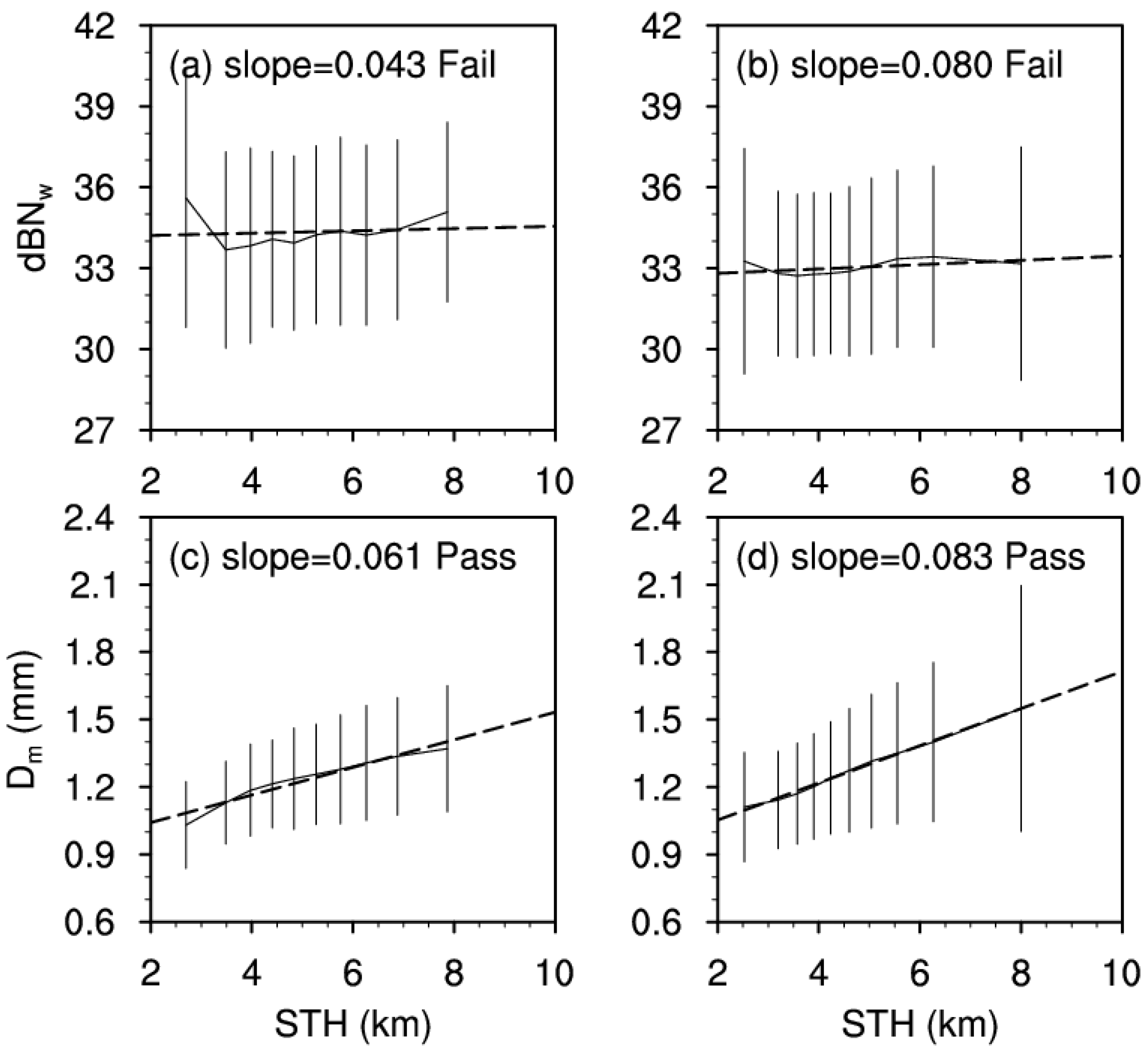
3.2. Relationship between Convective Intensity Indicators and DSDs

Next, we included the CTH from FY-4A observations to explore the ability of various parameters to serve as indicators of the surface DSD during the 2020-TC period. Figure 9 shows the relationship between both CTH and CTH-STH and near-surface DSD. CTH is positively correlated with near-surface dBNw and passes the 95% significance test (Figure 9a), while CTH-STH appears to be independent of dBNw (Figure 9b). In contrast, CTH is independent of Dm (Figure 9c), but CTH-STH is negatively correlated with Dm and passes the significance test (Figure 9d). The above results show that CTH, as an indicator of convection intensity, actually characterizes more raindrop concentrations. CTH-STH can indeed be used to approximate the intensity of convection [25], because it can indicate the near-surface raindrop size.
One possible explanation for the above phenomenon is that strong convection is better able to transport larger particles and/or more hydrometeors to higher altitudes, while bringing about more latent heat release and accelerating updrafts [17], resulting in higher CTH. This can also explain the negative correlation in Figure 9d, as the smaller difference between CTH and STH indicates that more large particles are lifted by the strong upward motion [25], while promoting the rapid growth of graupel rather than snow [30]. As a result, particles falling to the surface appear larger. However, there is still a problem here, which is that high STH and CTH both indicate intense convection, but their relationship with DSD is significantly different (e.g., Figure 7c shows that only the relationship between STH and Dm passes the significance test, while Figure 9a shows that only the relationship between CTH and dBNw passes the significance test).
To explore this issue in depth, we classified the precipitation based on the dominant microphysical processes below the melting level, following the approach used in Figure 8, and calculated the relationship between three indicators and the near-surface DSD (Figure 10 and Figure 11). From top to bottom, they correspond to the four quadrants (coalescence, size-sorting or evaporation, break-up, and break-up and coalescence balance) shown in Figure 8. An interesting phenomenon is that, unlike Figure 7a (the relationship between STH and dBNw fails the significance test), Figure 10d,g,j shows that the positive relationship between STH and dBNw passes the significance test, and the slopes are 0.305, 0.273, and 0.245. Although the relationship between CTH and dBNw passes the significance test (Figure 9a), Figure 10e,h,k shows larger slopes. No matter what microphysical processes exist in the liquid phase, the relationship between CTH-STH and dBNw is not significant. This phenomenon suggests that coalescence in the low level interferes with the indication of raindrop concentration by STH and CTH, because the process is very complex—on the one hand, raindrops merge to reduce the concentration, and on the other hand, the reduction in the condensation surface area increases the level of supersaturation, activating new condensation nuclei and causing an increase in raindrop concentration. The second quadrant (size-sorting or evaporation) shows the strongest positive correlation, whether it is STH vs. dBNw or CTH vs. dBNw, which may be because evaporation usually occurs after raindrops have left the cloud. The effect of evaporation on raindrops is easier to describe, so STH and CTH are good indicators of the near-surface raindrop concentration in this case.
Unlike the raindrop concentration, no matter what the dominant microphysical process below the melting level is, there is a positive correlation between STH and Dm that passes the significance test, and the slopes are similar (0.063–0.069). It is worth noting that while Figure 9c shows that CTH is independent of Dm, a negative correlation that passes the significance test appears in Figure 11e. That is, in the dominant microphysical process of size-sorting or evaporation, the higher the CTH, the smaller the Dm. We suspect that there may have been a multi-layer cloud structure. This speculation can be seen from the distribution of STH, which it is mostly concentrated below 6 km. The upper cloud layer may have been the cloud cover advecting from the strong TC convection area, which does not actually produce precipitation, while the lower cloud layer would have been the shallow convection that produced the precipitation. Stephens and Wood (2007) found a similar phenomenon in tropical convection, and they pointed out that the top of the upper cloud is usually up to 12 km, but the actual precipitation layer is located slightly above the melting level [49]. CTH-STH also shows a consistent negative correlation with Dm and passes the significance test, indicating that it is effective as an indicator of surface Dm.

4. Discussion

Compared with September 2014–September 2019, in the ice-phase region, the precipitation in Northeast China during the 2020-TC period has stronger precipitation ice productivity, weaker deposition efficiency, and a stronger riming process. The arrival of the TCs raises the melting level, such that the 2020-TC precipitation has a broader space for the development of warm rain processes. The average surface dBNw and Dm are 34.4 (33.0) and 1.23 (1.28) mm for 2020-TC (September 2014–September 2019), respectively. This is close to the DSD of stratiform precipitation reported by Bringi et al. (2003) [46], and has smaller dBNw and Dm than landfalling TCs in other parts of China.
When the liquid-phase processes were not distinguished, the relationships between STH (CTH) and Dm (dBNw) were itemized as follows:
-
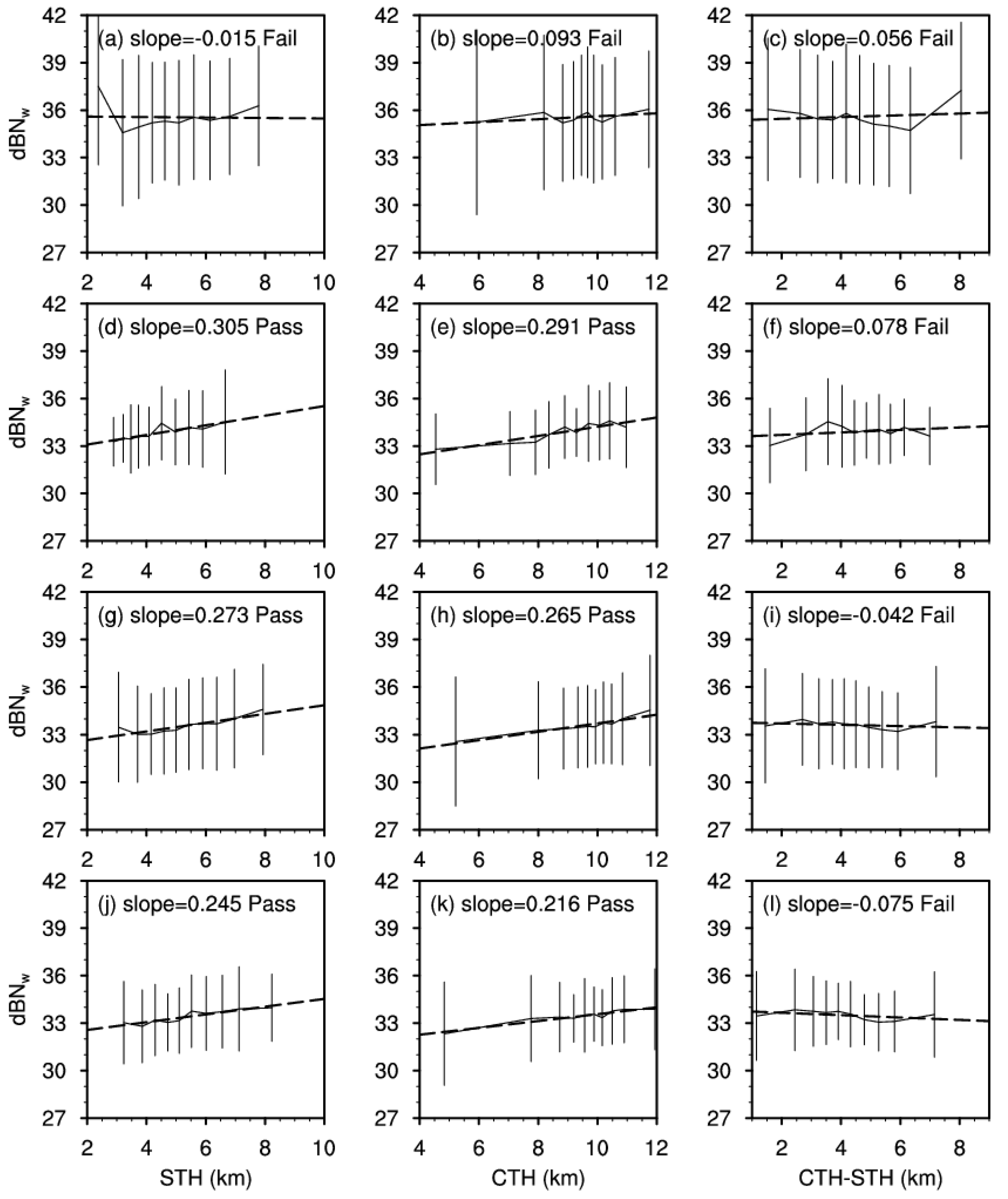
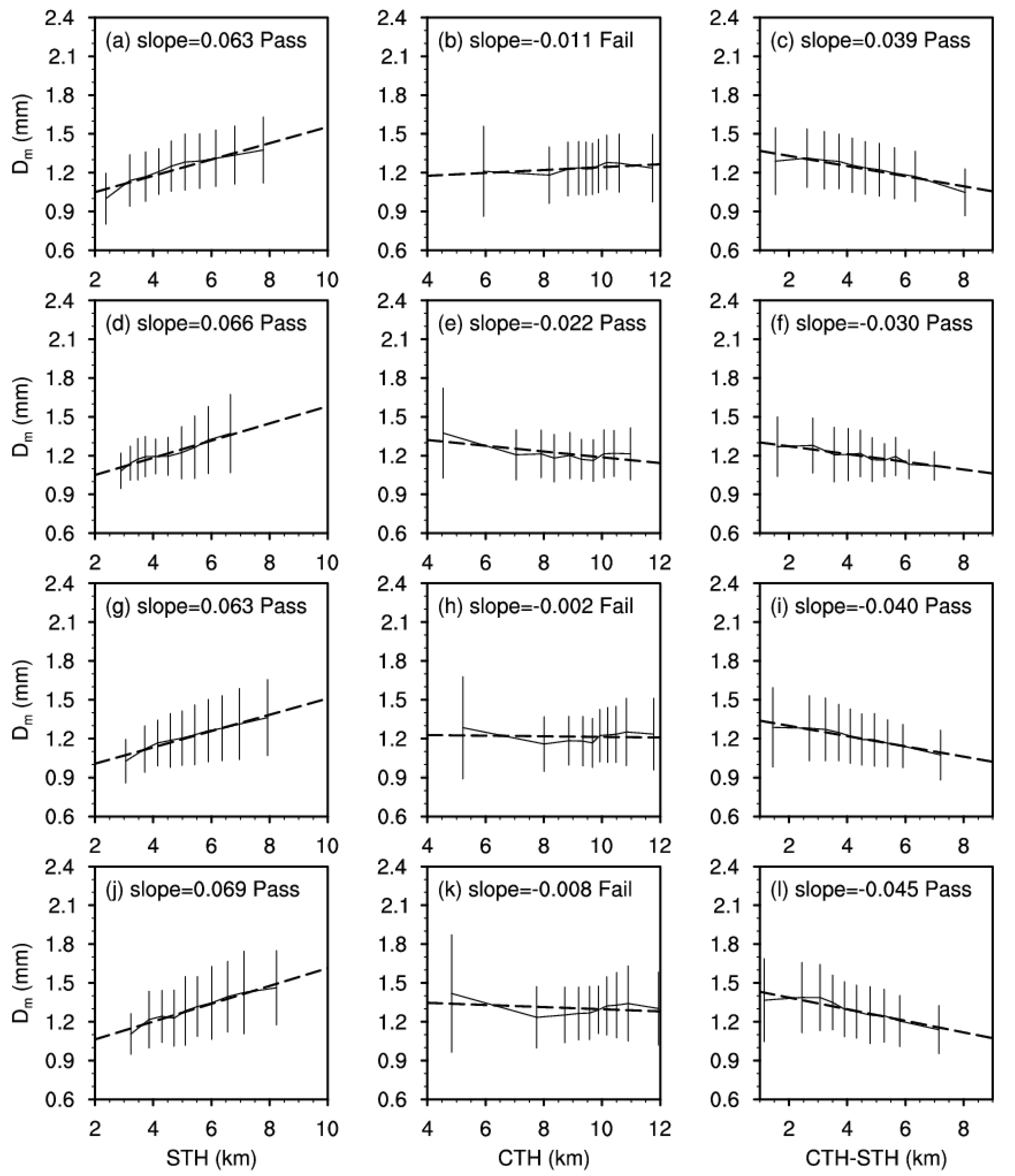
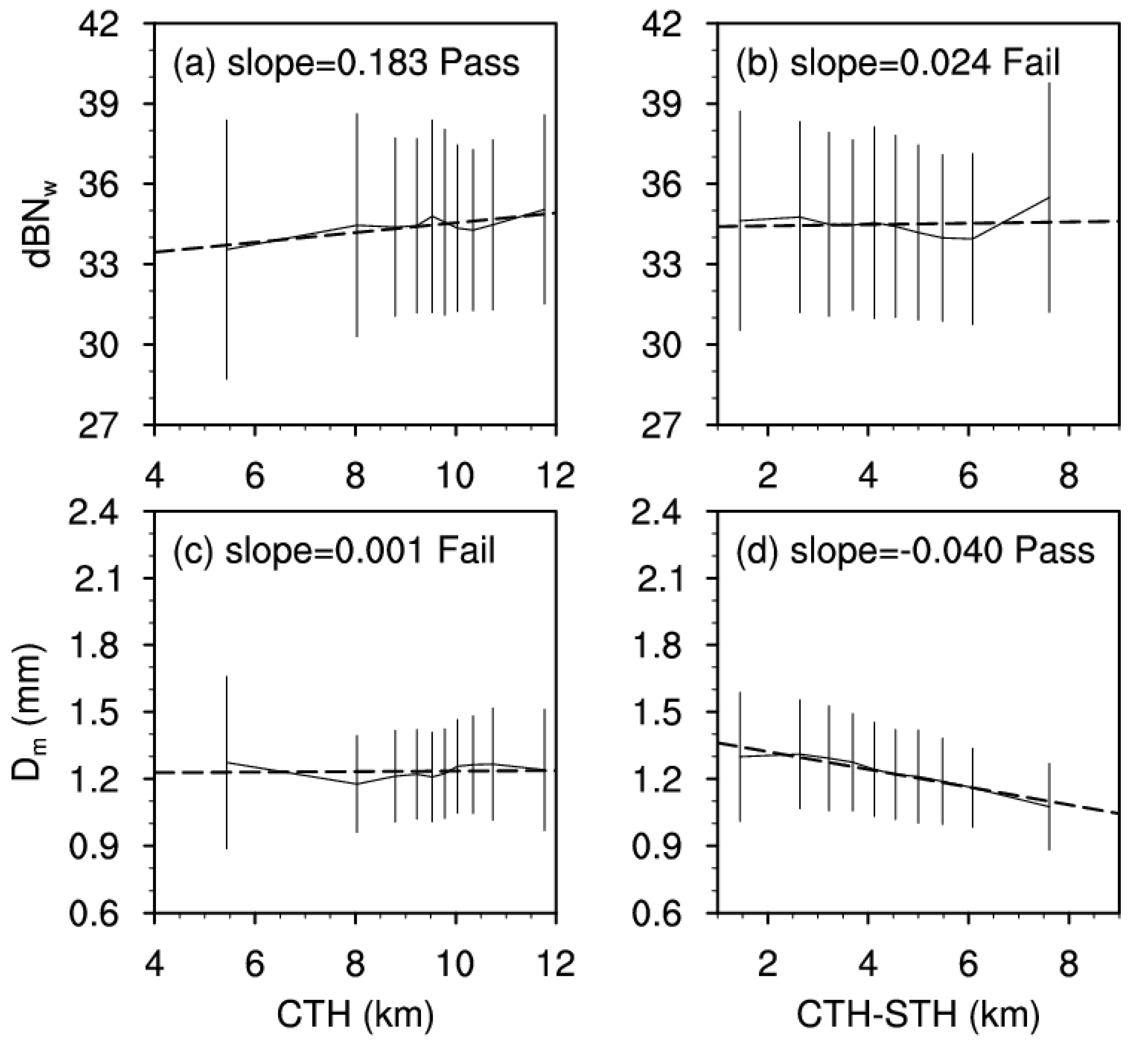
Positive correlation between STH and Dm passes the test.
-
Positive correlation between CTH and dBNw passes the test.
-
Negative correlation between CTH-STH and Dm passes the test.
-
The other relationships all fail the test.
Compared with September 2014–September 2019, the Dm of 2020-TC increases relatively slowly with STH, indicating the influence of complex microphysical processes. Coalescence is the dominant liquid-phase microphysical process (46%) of precipitation in 2020-TC, but its proportion is much lower than that of TC precipitation in other regions. In addition, 2020-TC has less size-sorting and evaporation than the precipitation in September 2014–September 2019.
When the liquid-phase processes were distinguished, the important relationships between STH (CTH) and Dm (dBNw) were itemized as follows:
-
Positive correlations of STH (CTH) with dBNw pass the test (except coalescence).
-
The relationships between STH (CTH) and dBNw fail the test (coalescence dominant).
-
The relationships between STH and Dm pass the test (any conditions).
-
Negative correlation between CTH and Dm passes the test (size-sorting or evaporation).
-
The relationship between CTH-STH and DSD is the same as when liquid-phase processes are not distinguished.
There is a long-standing discussion on the effects of STH and CTH on near-surface precipitation. For example, Hamada et al. (2015) concluded a weak linkage between the heaviest rainfall and tallest storms [50], while Wang and Tang (2020) found strong positive relationships between extreme convection and precipitation [51]. In this paper, using the GPM 2ADPR, the precipitation intensity was split into two relatively independent variables, dBNw and Dm, and the relationships between STH (CTH) and Dm (dBNw) were discussed. Liu et al. (2007) proposed CTH-STH as a proxy of convection intensity [25]. Here, we found that this variable can indeed indicate the surface Dm. However, given that this variable requires observations with two instruments (infrared and radar) simultaneously, in practical terms, it may be difficult to use.
The GPM core satellite, equipped with a unique DPR instrument, provides DSD data for areas deficient in ground-based observations. FY-4A, as a stationary satellite, can achieve continuous observation of the hemisphere. Combining GPM DPR and FY-4A AGRI data provides an excellent opportunity to study microphysical structures. In this paper, we focused on the microphysical characteristics of landfalling TCs in Northeast China in 2020, and attempted to reveal the relationship between near-surface DSD and parameters characterizing convection intensity (STH, CTH, and CTH-STH). It is concluded that the DSD of TCs in Northeast China is different from that of local precipitation and landfalling TC precipitation in other regions. Rain top and cloud top indicate raindrop diameter and concentration, respectively. Elucidating the microphysical processes that cause this difference in even more detail depends on further observational studies and high-resolution numerical simulations being conducted in the future.

Author Contributions

A.Z. and Y.C. conceived the idea and proposed this study. Y.C. prepared the data and drafted the manuscript. X.P., S.C., Y.H., and W.L. discussed the concepts and edited the manuscript. All authors have read and agreed to the published version of the manuscript.

Funding

This work was funded by the Guangdong Major Project of Basic and Applied Basic Research (grant number 2020B0301030004), the National Natural Science Foundation of China (grant numbers 42105068, 42075004, and 42005062), the Fengyun Application Pioneering Project (grant number FY-APP-2021.0114), and the Innovation Group Project of Southern Marine Science and Engineering Guangdong Laboratory (Zhuhai) (grant number 311021009).

Institutional Review Board Statement

Not applicable.

Informed Consent Statement

Not applicable.

Data Availability Statement

The GPM 2ADPR dataset used in this study was collected from the Precipitation Measurement Mission website: https://pmm.nasa.gov (accessed on 2 March 2022). The FY-4A dataset used in this study was collected from: http://data.nsmc.org.cn/. The Himawari-8 CTH used in this study was collected from: ftp.ptree.jaxa.jp (accessed on 2 March 2022).

Conflicts of Interest

The authors declare no conflict of interest.

References

  1. Chang, W.Y.; Wang, T.C.C.; Lin, P.L. Characteristics of the Raindrop Size Distribution and Drop Shape Relation in Typhoon Systems in the Western Pacific from the 2D Video Disdrometer and NCU C-Band Polarimetric Radar. J. Atmos. Ocean. Technol. 2009, 26, 1973–1993. [Google Scholar] [CrossRef]
  2. Morrison, H.; Thompson, G.; Tatarskii, V. Impact of Cloud Microphysics on the Development of Trailing Stratiform Precipitation in a Simulated Squall Line: Comparison of One- and Two-Moment Schemes. Mon. Weather Rev. 2009, 137, 991–1007. [Google Scholar] [CrossRef] [Green Version]
  3. Chen, Y.; Duan, J.; An, J.; Liu, H. Raindrop Size Distribution Characteristics for Tropical Cyclones and Meiyu-Baiu Fronts Impacting Tokyo, Japan. Atmosphere 2019, 10, 391. [Google Scholar] [CrossRef] [Green Version]
  4. Janapati, J.; Seela, B.K.; Lin, P.-L.; Lee, M.-T.; Joseph, E. Microphysical features of typhoon and non-typhoon rainfall observed in Taiwan, an island in the northwestern Pacific. Hydrol. Earth Syst. Sci. 2021, 25, 4025–4040. [Google Scholar] [CrossRef]
  5. Wang, M.J.; Zhao, K.; Lee, W.C.; Zhang, F.Q. Microphysical and Kinematic Structure of Convective-Scale Elements in the Inner Rainband of Typhoon Matmo (2014) After Landfall. J. Geophys. Res.-Atmos. 2018, 123, 6549–6564. [Google Scholar] [CrossRef] [Green Version]
  6. Wang, M.J.; Zhao, K.; Xue, M.; Zhang, G.F.; Liu, S.; Wen, L.; Chen, G. Precipitation microphysics characteristics of a Typhoon Matmo (2014) rainband after landfall over eastern China based on polarimetric radar observations. J. Geophys. Res.-Atmos. 2016, 121, 12415–12433. [Google Scholar] [CrossRef]
  7. Wen, L.; Zhao, K.; Chen, G.; Wang, M.; Zhou, B.; Huang, H.; Hu, D.; Lee, W.-C.; Hu, H. Drop Size Distribution Characteristics of Seven Typhoons in China. J. Geophys. Res.-Atmos. 2018, 123, 6529–6548. [Google Scholar] [CrossRef]
  8. Zheng, H.P.; Zhang, Y.; Zhang, L.F.; Lei, H.C.; Wu, Z.H. Precipitation Microphysical Processes in the Inner Rainband of Tropical Cyclone Kajiki (2019) over the South China Sea Revealed by Polarimetric Radar. Adv. Atmos. Sci. 2021, 38, 65–80. [Google Scholar] [CrossRef]
  9. Duan, Y.H.; Wan, Q.L.; Huang, J.; Huang, J.; Zhao, K.; Yu, H.; Wang, Y.; Zhao, D.; Feng, J.; Tang, J.; et al. Landfalling Tropical Cyclone Research Project (LTCRP) in China. Bull. Am. Meteorol. Soc. 2019, 100, Es447–Es472. [Google Scholar] [CrossRef]
  10. Jones, S.C.; Harr, P.A.; Abraham, J.; Bosart, L.F.; Bowyer, P.J.; Evans, J.L.; Hanley, D.E.; Hanstrum, B.N.; Hart, R.E.; Lalaurette, F.; et al. The extratropical transition of tropical cyclones: Forecast challenges, current understanding, and future directions. Weather. Forecast. 2003, 18, 1052–1092. [Google Scholar] [CrossRef]
  11. Wang, H.; Wang, W.Q.; Wang, J.; Gong, D.L.; Zhang, D.G.; Zhang, L.; Zhang, Q.C. Rainfall Microphysical Properties of Landfalling Typhoon Yagi (201814) Based on the Observations of Micro Rain Radar and Cloud Radar in Shandong, China. Adv. Atmos. Sci. 2021, 38, 994–1011. [Google Scholar] [CrossRef]
  12. Hou, A.Y.; Kakar, R.K.; Neeck, S.; Azarbarzin, A.A.; Kummerow, C.D.; Kojima, M.; Oki, R.; Nakamura, K.; Iguchi, T. The Global Precipitation Measurement Mission. Bull. Am. Meteorol. Soc. 2014, 95, 701–722. [Google Scholar] [CrossRef]
  13. Huang, H.; Chen, F. Precipitation Microphysics of Tropical Cyclones Over the Western North Pacific Based on GPM DPR Observations: A Preliminary Analysis. J. Geophys. Res.-Atmos. 2019, 124, 3124–3142. [Google Scholar] [CrossRef]
  14. Chen, F.J.; Fu, Y.F.; Yang, Y.J. Regional Variability of Precipitation in Tropical Cyclones Over the Western North Pacific Revealed by the GPM Dual-Frequency Precipitation Radar and Microwave Imager. J. Geophys. Res.-Atmos. 2019, 124, 11281–11296. [Google Scholar] [CrossRef]
  15. Wu, Z.; Huang, Y.; Zhang, Y.; Zhang, L.; Lei, H.; Zheng, H. Precipitation characteristics of typhoon Lekima (2019) at landfall revealed by joint observations from GPM satellite and S-band radar. Atmos. Res. 2021, 260, 105714. [Google Scholar] [CrossRef]
  16. Huang, H.; Zhao, K.; Fu, P.L.; Chen, H.N.; Chen, G.; Zhang, Y. Validation of Precipitation Measurements from the Dual-Frequency Precipitation Radar Onboard the GPM Core Observatory Using a Polarimetric Radar in South China. IEEE Trans. Geosci. Remote Sens. 2022, 60, 4104216. [Google Scholar] [CrossRef]
  17. Luo, Z.J.; Jeyaratnam, J.; Iwasaki, S.; Takahashi, H.; Anderson, R. Convective vertical velocity and cloud internal vertical structure: An A-Train perspective. Geophys. Res. Lett. 2014, 41, 723–729. [Google Scholar] [CrossRef]
  18. Huo, J.; Lu, D.R.; Duan, S.; Bi, Y.H.; Liu, B. Comparison of the cloud top heights retrieved from MODIS and AHI satellite data with ground-based Ka-band radar. Atmos. Meas. Tech. 2020, 13, 1–11. [Google Scholar] [CrossRef] [Green Version]
  19. Liu, C.Y.; Chiu, C.H.; Lin, P.H.; Min, M. Comparison of Cloud-Top Property Retrievals from Advanced Himawari Imager, MODIS, CloudSat/CPR, CALIPSO/CALIOP, and Radiosonde. J. Geophys. Res.-Atmos. 2020, 125, e2020JD032683. [Google Scholar] [CrossRef]
  20. Yang, X.; Ge, J.M.; Hu, X.Y.; Wang, M.H.; Han, Z.H. Cloud-Top Height Comparison from Multi-Satellite Sensors and Ground-Based Cloud Radar over SACOL Site. Remote Sens. 2021, 13, 2715. [Google Scholar] [CrossRef]
  21. Sun, L.X.; Tang, X.D.; Zhuge, X.Y.; Tan, Z.M.; Fang, J. Diurnal Variation of Overshooting Tops in Typhoons Detected by Himawari-8 Satellite. Geophys. Res. Lett. 2021, 48, e2021GL095565. [Google Scholar] [CrossRef]
  22. Masunaga, H.; Kummerow, C.D. Observations of tropical precipitating clouds ranging from shallow to deep convective systems. Geophys. Res. Lett. 2006, 33, L16805. [Google Scholar] [CrossRef] [Green Version]
  23. Masunaga, H.; L’Ecuyer, T.S.; Kummerow, C.D. Variability in the characteristics of precipitation systems in the tropical Pacific. Part 1: Spatial structure. J. Clim. 2005, 18, 823–840. [Google Scholar] [CrossRef] [Green Version]
  24. Masunaga, H.; Satoh, M.; Miura, H. A joint satellite and global cloud-resolving model analysis of a Madden-Julian Oscillation event: Model diagnosis. J. Geophys. Res.-Atmos. 2008, 113, D17210. [Google Scholar] [CrossRef] [Green Version]
  25. Liu, C.T.; Zipser, E.J.; Nesbitt, S.W. Global distribution of tropical deep convection: Different perspectives from TRMM infrared and radar data. J. Clim. 2007, 20, 489–503. [Google Scholar] [CrossRef]
  26. Smalley, K.M.; Rapp, A.D. A-Train estimates of the sensitivity of the cloud-to-rainwater ratio to cloud size, relative humidity, and aerosols. Atmos. Chem. Phys. 2021, 21, 2765–2779. [Google Scholar] [CrossRef]
  27. Takayabu, Y.N. Spectral representation of rain profiles and diurnal variations observed with TRMM PR over the equatorial area. Geophys. Res. Lett. 2002, 29, 1584. [Google Scholar] [CrossRef] [Green Version]
  28. McFarquhar, G.M.; Jewett, B.F.; Gilmore, M.S.; Nesbitt, S.W.; Hsieh, T.L. Vertical Velocity and Microphysical Distributions Related to Rapid Intensification in a Simulation of Hurricane Dennis (2005). J. Atmos. Sci. 2012, 69, 3515–3534. [Google Scholar] [CrossRef]
  29. Chen, Y.L.; Zhang, A.Q.; Zhang, Y.H.; Cui, C.G.; Wan, R.; Wang, B.; Fu, Y.F. A Heavy Precipitation Event in the Yangtze River Basin Led by an Eastward Moving Tibetan Plateau Cloud System in the Summer of 2016. J. Geophys. Res.-Atmos. 2020, 125, e2020JD032429. [Google Scholar] [CrossRef]
  30. Dodson, J.B.; Taylor, P.C.; Branson, M. Microphysical variability of Amazonian deep convective cores observed by CloudSat and simulated by a multi-scale modeling framework. Atmos. Chem. Phys. 2018, 18, 6493–6510. [Google Scholar] [CrossRef] [Green Version]
  31. Lu, X.Q.; Yu, H.; Ying, M.; Zhao, B.; Zhang, S.; Lin, L.; Bai, L.; Wan, L. Western North Pacific Tropical Cyclone Database Created by the China Meteorological Administration. Adv. Atmos. Sci. 2021, 38, 690–699. [Google Scholar] [CrossRef]
  32. Speirs, P.; Gabella, M.; Berne, A. A comparison between the GPM dual-frequency precipitation radar and ground-based radar precipitation rate estimates in the Swiss Alps and Plateau. J. Hydrometeorol. 2017, 18, 1247–1269. [Google Scholar] [CrossRef]
  33. Petracca, M.; D’Adderio, L.P.; Porcù, F. Validation of GPM dual-frequency precipitation radar (DPR) rainfall products over Italy. J. Hydrometeorol. 2018, 19, 907–925. [Google Scholar] [CrossRef]
  34. D’Adderio, L.P.; Vulpiani, G.; Porcù, F.; Tokay, A.; Meneghini, R. Comparison of GPM core observatory and ground-based radar retrieval of mass-weighted mean raindrop diameter at midlatitude. J. Hydrometeorol. 2018, 19, 1583–1598. [Google Scholar] [CrossRef]
  35. Ryu, J.; Song, H.J.; Sohn, B.J.; Liu, C. Global Distribution of Three Types of Drop Size Distribution Representing Heavy Rainfall From GPM/DPR Measurements. Geophys. Res. Lett. 2021, 48, e2020GL090871. [Google Scholar] [CrossRef]
  36. Seto, S.; Iguchi, T.; Meneghini, R.; Awaka, J.; Kubota, T.; Masaki, T.; Takahashi, N. The Precipitation Rate Retrieval Algorithms for the GPM Dual-frequency Precipitation Radar. J. Meteorol. Soc. Jpn. 2021, 99, 205–237. [Google Scholar] [CrossRef]
  37. Zhang, C.; Zhang, Q.; Wang, Y.; Liang, X. Climatology of warm season cold vortices in East Asia: 1979–2005. Meteorol. Atmos. Phys. 2008, 100, 291–301. [Google Scholar] [CrossRef]
  38. Yang, J.; Zhang, Z.Q.; Wei, C.Y.; Lu, F.; Guo, Q. Introducing the New Generation of Chinese Geostationary Weather Satellites, Fengyun-4. Bull. Am. Meteorol. Soc. 2017, 98, 1637–1658. [Google Scholar] [CrossRef]
  39. Min, M.; Wu, C.Q.; Li, C.; Liu, H.; Xu, N.; Wu, X.; Chen, L.; Wang, F.; Sun, F.; Qin, D.; et al. Developing the Science Product Algorithm Testbed for Chinese Next-Generation Geostationary Meteorological Satellites: Fengyun-4 Series. J. Meteorol. Res. 2017, 31, 708–719. [Google Scholar] [CrossRef]
  40. Chen, Y.L.; Li, W.B.; Chen, S.M.; Zhang, A.Q.; Fu, Y.F. Linkage Between the Vertical Evolution of Clouds and Droplet Growth Modes as Seen From FY-4A AGRI and GPM DPR. Geophys. Res. Lett. 2020, 47, e2020GL088312. [Google Scholar] [CrossRef]
  41. Xu, W.J.; Lyu, D.R. Evaluation of Cloud Mask and Cloud Top Height from Fengyun-4A with MODIS Cloud Retrievals over the Tibetan Plateau. Remote Sens. 2021, 13, 1418. [Google Scholar] [CrossRef]
  42. Zagrodnik, J.P.; McMurdie, L.A.; Houze, R.A.; Tanelli, S. Vertical Structure and Microphysical Characteristics of Frontal Systems Passing over a Three-Dimensional Coastal Mountain Range. J. Atmos. Sci. 2019, 76, 1521–1546. [Google Scholar] [CrossRef]
  43. Zagrodnik, J.P.; McMurdie, L.A.; Houze, R.A. Stratiform Precipitation Processes in Cyclones Passing over a Coastal Mountain Range. J. Atmos. Sci. 2018, 75, 983–1004. [Google Scholar] [CrossRef] [Green Version]
  44. Bao, X.W.; Wu, L.G.; Zhang, S.; Li, Q.; Lin, L.; Zhao, B.; Wu, D.; Xia, W.; Xu, B. Distinct Raindrop Size Distributions of Convective Inner- and Outer-Rainband Rain in Typhoon Maria (2018). J. Geophys. Res.-Atmos. 2020, 125, e2020JD032482. [Google Scholar] [CrossRef]
  45. Bao, X.W.; Wu, L.G.; Zhang, S.; Yuan, H.Z.; Wang, H.H. A Comparison of Convective Raindrop Size Distributions in the Eyewall and Spiral Rainbands of Typhoon Lekima (2019). Geophys. Res. Lett. 2020, 47, e2020GL090729. [Google Scholar] [CrossRef]
  46. Bringi, V.N.; Chandrasekar, V.; Hubbert, J.; Gorgucci, E.; Randeu, W.L.; Schoenhuber, M. Raindrop size distribution in different climatic regimes from disdrometer and dual-polarized radar analysis. J. Atmos. Sci. 2003, 60, 354–365. [Google Scholar] [CrossRef]
  47. Han, B.; Du, Y.; Wu, C.; Liu, X. Microphysical Characteristics of the Coexisting Frontal and Warm-Sector Heavy Rainfall in South China. J. Geophys. Res.-Atmos. 2021, 126, e2021JD035446. [Google Scholar] [CrossRef]
  48. Kumjian, M.R.; Prat, O.P. The Impact of Raindrop Collisional Processes on the Polarimetric Radar Variables. J. Atmos. Sci. 2014, 71, 3052–3067. [Google Scholar] [CrossRef]
  49. Stephens, G.L.; Wood, N.B. Properties of tropical convection observed by millimeter-wave radar systems. Mon. Weather. Rev. 2007, 135, 821–842. [Google Scholar] [CrossRef]
  50. Hamada, A.; Takayabu, Y.N.; Liu, C.; Zipser, E.J. Weak linkage between the heaviest rainfall and tallest storms. Nat. Commun. 2015, 6, 6213. [Google Scholar] [CrossRef]
  51. Wang, T.C.; Tang, G.Q. Spatial Variability and Linkage between Extreme Convections and Extreme Precipitation Revealed by 22-Year Space-Borne Precipitation Radar Data. Geophys. Res. Lett. 2020, 47, e2020GL088437. [Google Scholar] [CrossRef]
Figure 1. Three TCs that affected Northeast China in 2020. The numbers represent the dates; the large black dots represent 0000 UTC; the small black dots represent 6-h intervals; the colors represent the central maximum wind speed. The data source is the Western North Pacific Tropical Cyclone Database produced by the China Meteorological Administration [31].
Remotesensing 14 02188 g001
Figure 2. Example of the quasi-simultaneous observations of MODIS, FY-4A, and Himawari-8 in the study area at 05:15, 05:15, and 05:10 UTC on 8 September 2020, respectively. The black dashed lines in (b) and (c) are the orbital boundaries of MODIS in (a).
Remotesensing 14 02188 g002
Figure 3. Pixel-to-pixel comparison of FY-4A CTH with (a) MODIS CTH and (b) Himawari-8 CTH. The timespan used for the statistics is from 2 to 9 September 2020, in which Himawari-8 only has daytime data. The color fill is the occurrence probability of each bin, and the bin interval is 0.5 km.
Remotesensing 14 02188 g003
Figure 4. CFADs for the reflectivity during the (a) 2020-TC period, (b) September 2014–September 2019 period, and (c) their difference (former minus the latter). The CFADs are normalized by the overall maximum, and the value of each bin represents the occurrence frequency compared to the absolute maximum frequency.
Remotesensing 14 02188 g004
Figure 5. PDFs of near-surface DSD for (a) 2020-TC, (b) September 2014–September 2019, and (c) their difference (former minus the latter). The PDF is normalized with the overall maximum, and the value of each bin represents the occurrence frequency compared to the absolute maximum frequency: 100% is equivalent to 6201 observations in (a) and 44,875 observations in (b). The Dm interval is 0.2 mm, and the dBNw interval is 2. Dashed line and solid line boxes represent “maritime-like” cluster and “continental-like” cluster proposed by reference [44], respectively.
Remotesensing 14 02188 g005
Figure 6. Vertical profiles for (a) dBNw and (b) Dm. The blue line represents the 2020-TC period, and the red line represents the September 2014–September 2019 period.
Remotesensing 14 02188 g006
Figure 7. Relationship between STH and DSD: (a,b) STH vs. dBNw; (c,d) STH vs. Dm; (a,c) 2020-TC; (b,d) September 2014–September 2019. Bars represent the standard deviation; the dashed line is the line of best fit for 10 equal-sample points; the panel lettering of each sub-figure is followed by the slope of the line of best fit and whether it passes the 95% significance test.
Remotesensing 14 02188 g007
Figure 8. Frequency patterns in two-dimensional space of ΔDm and ΔReflectivity for (a) 2020-TC, (b) September 2014–September 2019, and (c) their difference (former minus the latter). The text in the figure represents the dominant microphysical processes and proportions in each quadrant.
Remotesensing 14 02188 g008
Figure 9. Relationship of (a,c) CTH and (b,d) CTH-STH with (a,b) dBNw and (c,d) Dm for 2020-TC. Bars represent the standard deviation; the dashed line is the line of best fit for 10 equal-sample points; the panel lettering of each sub-figure is followed by the slope of the line of best fit and whether it passes the 95% significance test.
Remotesensing 14 02188 g009
Figure 10. Relationship of STH (left), CTH (middle), and CTH-STH (right) with dBNw during the 2020-TC period. According to the classification shown in Figure 8, the different dominant physical processes under the melting level are represented from top to bottom: (ac) coalescence, (df) size-sorting or evaporation, (gi) break-up, and (jl) break-up and coalescence balance. Bars represent the standard deviation; the dashed line is the line of best fit for 10 equal-sample points; the panel lettering of each sub-figure is followed by the slope of the line of best fit and whether it passes the 95% significance test.
Remotesensing 14 02188 g010
Figure 11. Relationship of STH (left), CTH (middle), and CTH-STH (right) with Dm during the 2020-TC pe-riod. According to the classification shown in Figure 8, the different dominant physical processes under the melting level are represented from top to bottom: (ac) coalescence, (df) size-sorting or evaporation, (gi) break-up, and (jl) break-up and coalescence balance. Bars represent the standard deviation; the dashed line is the line of best fit for 10 equal-sample points; the panel let-tering of each sub-figure is followed by the slope of the line of best fit and whether it passes the 95% significance test.
Remotesensing 14 02188 g011
Publisher’s Note: MDPI stays neutral with regard to jurisdictional claims in published maps and institutional affiliations.

