Article

Monitoring Annual Land Use/Land Cover Change in the Tucson Metropolitan Area with Google Earth Engine (1986–2020)

by
Fabrice Dubertret
1,*,
François-Michel Le Tourneau
2,
Miguel L. Villarreal
3 and
Laura M. Norman
4
1
International Research Laboratory on Interdisciplinary Global Environmental Studies (IRL iGLOBES), National Scientific Research Center (CNRS), University of Arizona, 845 N. Park Avenue, Marshall Building 5th Floor, Tucson, AZ 85719, USA
2
National Scientific Research Center (CNRS)—Pôle de Recherche pour l’Organisation et la Diffusion de l’Information Géographique (PRODIG), Campus Condorcet, Bâtiment Recherche Sud, 5 Cours des Humanités, 93300 Aubervilliers, France
3
U.S. Geological Survey, Western Geographic Science Center, Moffett Field, CA 94035, USA
4
U.S. Geological Survey, Western Geographic Science Center, Tucson, AZ 85719, USA
*
Author to whom correspondence should be addressed.
Remote Sens. 2022, 14(9), 2127; https://doi.org/10.3390/rs14092127
Submission received: 27 January 2022 / Revised: 19 April 2022 / Accepted: 26 April 2022 / Published: 28 April 2022

Abstract

:
The Tucson metropolitan area, located in the Sonoran Desert of southeastern Arizona (USA), is affected by both massive population growth and rapid climate change, resulting in important land use and land cover (LULC) changes. As its fragile arid ecosystem and scarce resources are increasingly under pressure, there is a crucial need to monitor such landscape transformations. For such ends, we propose a method to compute yearly 30 m resolution LULC maps of the region from 1986 to 2020, using a combination of Landsat imagery, derived transformation and indices, texture analysis and other ancillary data fed to a Random Forest classifier. The entire process was hosted in the Google Earth Engine with tremendous computing capacities that allowed us to process a large amount of data and to achieve high overall classification accuracy for each year, ranging from 86.7 to 96.3%. Conservative post-processing techniques were also used to mitigate the persistent confusions between the numerous isolated houses in the region and their desert surroundings and to smooth year-specific LULC changes in order to identify general trends. We then show that policies to lessen urban sprawl in the area had little effects and we provide an automated tool to continue monitoring such dynamics in the future.

1. Introduction

The city of Tucson and the upper Santa Cruz River valley are located in the southeastern corner of Arizona, a region undergoing rapid land use and land cover (LULC) changes. From an economy mostly based on agriculture and mining in the early 20th century, the development of aeronautic industries and services (such as the University of Arizona, Tucson, AZ, USA) in the 1960s and 1970s have led to a population boom in the area [1,2]. As the popularization of air conditioning allowed residents to tame the scorching climate of the Sonoran Desert, people increasingly moved to work or retire in the area, attracted by a sunny year-round climate and relatively affordable housing [1,3]. The result was an exponential demographic rise with double-digit growth rates, which continues today: Pima County’s population, where Tucson is located, grew from 141,216 in 1950 to 351,667 in 1970, 666,880 in 1990 and 1,043,433 in 2020 [4].
As a consequence, the Tucson region displays rapid urban [5] and exurban growth [6,7], with most people coming to southeastern Arizona favoring individual houses with garden in sprawling suburban areas over apartments in cities. This trend, associated with other human-driven LULC changes related to agriculture and mining, is putting greater pressure on the already scarce water resources and is increasing habitat fragmentation, creating new imbalances in the complex ecosystem of the Sonoran Desert [5,8,9,10,11,12]. Moreover, the region is undergoing significant climate change at the same time, mainly manifested by a rise in temperature, extended dry season and unpredictable rainfall patterns [13,14] with a greater frequency of extreme events [15].
In this context, there is an urgent need to monitor the temporal and spatial patterns of LULC changes and assess how the environment is responding to such transformations. Remote sensing is a practical and cost-efficient tool for such ends, as demonstrated by the growing number of studies on land cover monitoring. However, even when conducted over the same area, the limited set of land cover classes used in generalized regional or national scale approaches [16,17,18], coarse temporal resolution [19,20], limited time span [21,22] and/or the focus on specific topics (such as impervious surfaces [23] or cropland [24]) may restrain the possible uses of their derived datasets for finer analysis on specific areas. Still, this flourishing literature provides valuable insights for adapting methods and good practices for conducting annual LULC quantification and change analysis over other regions of interest with different needs. While focusing on the Tucson metropolitan area, this research aims to provide a generic and adaptative tool for producing yearly LULC maps over long time periods.
Achieving a multitemporal analysis over several decades requires overcoming numerous technical challenges, such as rectifying the differences between multiple sensors across different time periods, or addressing heterogeneous data quality and availability due to various factors, notably cloud cover [25,26]. Recent cloud computing and big data approaches [27,28] have brought new solutions to such problems, allowing researchers to assemble and process very large datasets composed of collections of remote sensing images and other ancillary data [29,30], thus potentially dramatically improving the performances of image classification and LULC analyses [31,32]. Rather than hand-picking a set of images with 5- to 10-year intervals, these new techniques now allow time-effective processing, development and analysis of vast, virtually seamless and high-resolution annual land cover map products [17,33] that can be updated each year.
Google Earth Engine (GEE) is an open access JavaScript Application Programming Interface (API) providing for such cloud computing approaches with a multi-petabyte catalog of remote sensing data allowing users to select and process enormous volumes of data, and has already proven its capacities for land cover classification and change detection [26,28,30,34,35,36,37,38,39,40]. This paper builds on these approaches to present a GEE workflow for generating annual land cover map products of the upper Santa Cruz watershed at 30 m spatial resolution and over a 35-year-long period (1986–2020), rejoining and expanding previous decadal LULC mapping efforts in the region [19]. The use of biannual Landsat pre-processed composites and a large number of image transformations, indices, texture analysis, ancillary data and post-processing techniques allowed us to achieve accurate yearly land cover classifications (overall accuracy > 86.7%). As our script can be used for automated classifications of oncoming years, this allows for precise monitoring of LULC changes past and future, which will be illustrated with a succinct analysis of urban sprawl dynamics in the region, i.e., the expansion of city footprints through the creation of new low density urban areas on surrounding undeveloped lands [41].
The GEE scripts associated with this study, designed to be generic enough for easy adaptation to other areas of interest with different needs, are openly accessible for re-use and modification [42].

2. Materials and Methods

2.1. Study Area

Our study area covers 15,867 km2 of the binational Santa Cruz watershed in southern Arizona, United States and northern Sonora, Mexico (Figure 1). Its climate is characterized by mild winter and high summer temperatures, and a bimodal precipitation pattern with a dry season in spring followed by the North American Monsoon. Climate change is impacting the area, both by an overall rise in temperature with a higher frequency of extreme heat and by less predictable rainfall patterns with extended droughts followed by flood events [13,14,15].
The watershed topography is characteristic of the Basin and Range Province. It is composed of multiple mountain chains with steep and narrow canyons separated by vast, flat and arid valleys. Elevation ranges from 525 to 2855 m above sea level and is one of the main drivers influencing natural land cover, creating concentric belts of vegetation around mountain summits. Ascending from the arid plains, largely dominated by shrublands interrupted by mesquite and cottonwood trees along the riverbanks, natural land cover evolves into grassland, followed by oak, juniper and pine woodlands, up to aspen and mixed conifer forests [46].
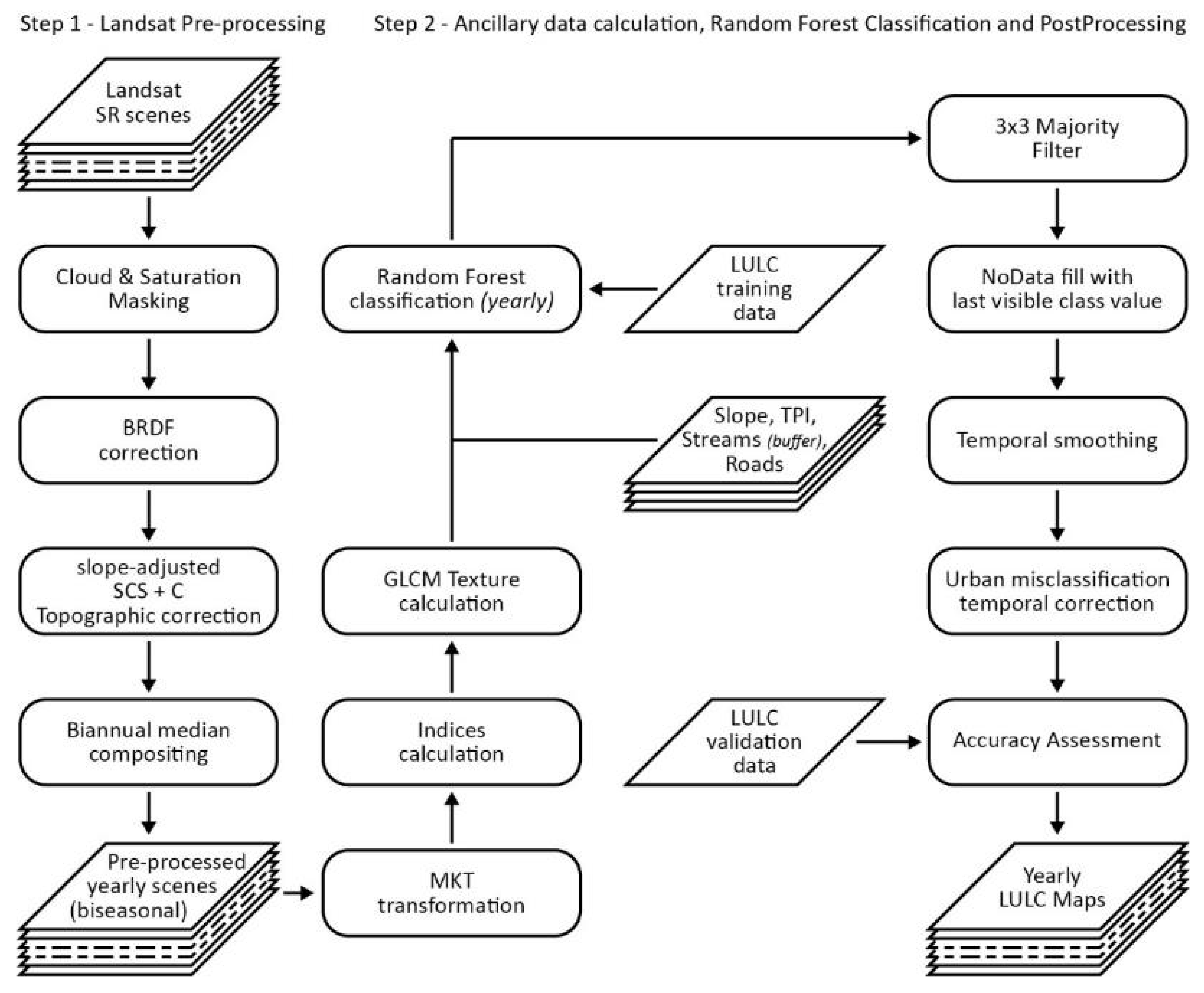
Two major urbanized areas are present in the upper Santa Cruz watershed (Figure 1): the rapidly growing Tucson metropolitan area and Ambos Nogales located on the United States–Mexico border [3,9,10,19,47,48]. While this study aims at expanding the temporal resolution of the decadal products by Villarreal et al. in 2011 [19], we also increased our coverage to include the catchment area of the upper Santa Cruz River up to its confluence with the Brawley Wash sub-basin which is also significantly affected by recent urban sprawl. The watershed boundaries used to define our region of interest were derived from the United States Geological Survey (USGS) National Hydrography Dataset Plus High Resolution [44], and used to clip all data used during our overall yearly LULC classification process (Figure 2).

2.2. Image Data and Pre-Processing

We chose to work with Landsat data, which provides imagery of the Earth’s surface for over 40 years at a medium/high spatial resolution of 30 m (60 m for the first satellites and thermal bands), in spectral bands which are generally consistent across the 8 different sensors launched since 1972, and will be in the next decades with the recent launch of Landsat 9. We used orthorectified and atmospherically corrected Landsat Surface Reflectance Tier 1 imagery collections available in Google Earth Engine for Landsat OLI/TIRS and TM sensors (Landsat ETM+ data were not used due to its Scan Line Corrector error). Clouds and saturated pixels were detected and masked using the associated quality band [49]. We expanded the cloud masks by 240 m to include possibly undetected fuzzy cloud edges and pixels affected by “adjacency effect”, i.e., light scattering around clouds disturbing the measurement of the surface reflectance [50]. Only scenes with cloud cover <25% were considered.
The large extent of the study area means that multiple Landsat scenes had to be used to get a full coverage, adding another point of complexity as these may be captured at different times and dates, which means that illumination conditions can be different (Landsat Path/Rows images needed to cover the entire study area are: 35/37, 35/38, 35/39, 36/37 and 36/38). To obtain seamless mosaics, we normalized reflectance values using Nadir Bidirectional Reflectance Distribution Function (BRDF) adjustment [51]. Regarding topographic corrections, we applied the well-performing Sun Canopy Sensor + C correction model [52,53,54] to each scene. However, to avoid problematic under or over-correction observed in steep slopes [55], we used a differentiated determination of the C parameter. Rather than processing the image as a whole, we thus divided the images in 16 different classes of slope (from 0° to 80° with 5° ranges) and computed a different C for each class. We also averaged the values of the two Landsat OLI thermal bands into a single band to ensure consistency with TM sensors.
These steps were applied on all available Landsat TM and OLI scenes over our study area for two time periods per year: one representing the dry early summer (1 May to 30 June) and one from the “green-up” or growing season that follows the monsoon (15 August to 31 October). For each, we composited the pre-processed Landsat scenes using the median value of each unmasked pixels, a method which has proven accuracy in processing time series data [26,30]. This allowed us to automatically get more than 99.3% coverage of our study area for both periods of each year between 1986 and 2021. Due to rare meteorological conditions, this percentage falls, however, to 97.6% in 1990. Additionally, no data allowing a relevant coverage of the study area for both seasons was available for years previous to 1986, nor for the year 2012 (because of Landsat 7 issues and the delayed launch of Landsat 8 from July 2011 to February 2013), which was thus left out of our time series. In summary, we used Landsat 5 TM imagery from 1986 to 2011 and Landsat 8 OLI imagery from 2013 to 2021.

2.3. Image Transformation and Ancillary Data

In order to improve the accuracy of the classification, we calculated a number of indices and gathered ancillary data. These derived datasets were subsequently included as new predictor variables in the yearly land cover classifications (Table 1).
Multitemporal Kauth-Thomas (MKT) transformations between the two periods of each year were computed using sensor-dependent coefficients found in the literature [64,65,66]. MKT transformation allows for a comparison between multidate datasets by producing a 12 bands matrix which contains 6 standard coefficients (greenness, wetness, brightness, and 3 “un-named” others) and their respective orthogonal change coefficients.
We derived Normalized Difference Vegetation Index (NDVI), Normalized Difference Water Index (NDWI), and several built-up and bareness indices from Landsat bands of both periods, namely the Normalized Difference Built-up Index (NDBI), the Built-up Area Extraction Index (BAEI), the Normalized Difference Bareness Index (NDBai), as well as the Dry Built-up and the Dry Bareness indices which are better performing in arid climates [56,57,58,59].
Gray-Level Co-occurrence Matrix (GLCM) textural features were then generated for every Landsat band, MKT transformation, and above-mentioned indices. Of the various GLCM-based textural features available, we only selected correlation and contrast, as recommended by Hall-Beyer [63] for simple texture analysis. As pointed out by the literature [58,63], kernel size is a critical parameter for texture classification as it defines the context around the reference pixel, and appropriate sizes must be based upon knowledge of the local geographical context and trial and error attempts. Out of numerous tests with various kernel sizes, alone or in combination, we found that a single 3 × 3 pixels window performed best in detecting (semi-) isolated housing which is characteristic of urban sprawl in the Tucson area. We used the average of 4 offset directions (0°, 45°, 90° and 135°) in our kernel to ensure directional independence of calculated texture features.
We also included other ancillary data as input for the classifier. Slope and a 15-pixel radius Topographic Position Index (TPI) for each pixel were derived from the Shuttle Radar Topography Mission (SRTM) 30 m resolution global digital elevation model [43]. TPI is a method of terrain classification which compares the elevation value of each cell against the mean elevation of its specified neighborhood [60,61,62]. We also used the USGS National Hydrography Dataset Plus High Resolution [44] Flowline data to calculate a buffer area around main streams proportional to the total drainage area (in km2) of each section with the formula:
buffer = log10 (Drainage Area) × 30 m
We extracted the main roads network (highways and trunk roads) from the OpenStreetMap [67] dataset and buffered it by 30 m. All these ancillary data were included as new bands in each annual dataset, which then grew to 124 bands each (Figure 2). This amount of data was only possible to handle using the supercomputer and parallel processing capabilities of GEE.

2.4. Training and Validation Data

Inspired by previous studies [19] and based on the National Land Cover Database [68,69], we defined a total of 14 major LULC classes. For classification purposes, some of these classes were subdivided in order to catch local variations in land cover spectral signature (Table 2). To ensure comparability with previous 1979 to 2009 decadal classifications [19], these subclasses were merged back into their parent wider classes when statistics were calculated (but detailed subclasses could be kept if need be).
As our goal was to use supervised classification algorithms, we created a set of 1923 polygons spread across our study area, totaling 10,579 hectares and representing all classes and subclasses (see Supplementary Materials Table S1 for detail). These polygons were drawn using a self-made grid mimicking Landsat pixel to ensure their homogeneity in composition, leading to heterogeneity in size. LULC class assignation for each polygon was conducted by a single trained interpreter, based on human visual analysis of different high resolution orthophoto sources, including National Agriculture Imagery Program (NAIP) aerial imagery or Google Earth current and historic repositories. The latter were used to ensure that these polygons had consistent LULC from 1986 to 2021, allowing us to use the same sample for each year. These “ground-truth” polygons were then randomly and equally split into training and validation datasets, later used to acquire a random stratified sample of 4874 training and 4960 validation points evenly distributed between our LULC classes and subclasses (about 277 points per class). Sampling was conducted at a minimum resolution of 30 m to ensure that two points could not fall within the same Landsat pixel.

2.5. Classification and Post-Processing

Each year’s 124 variable datasets and stratified sample training points were then provided as inputs for a supervised 10 trees Random Forest (RF) classification. RF is currently reported as one of the best classifiers, producing high accuracy while staying relatively computationally light [70,71,72,73]. RF classifications operate by constructing multiple decision trees and outputting for each pixel the mode of all predicted classes [74]. Thus, this method is less sensible to overfitting training data than single decision tree predictors, which they generally outperform [75]. This characteristic of RF classifiers and the tremendous computing capacities of GEE allowed us to feed all 124 variable datasets for the computation of LULC maps for each year, without the need for prior feature selection.
Yearly classified images produced by the RF classifier were cleaned using a majority filter with a 3 × 3 moving window to eliminate “salt-pepper” noise in the classification results and give it a smoother appearance. Remaining NoData pixels from each year’s cloud and saturation masks were filled with the last observed class value, or, if unavailable, with the next observable class value.
The whole 1986–2021 classification time series was then smoothed to reduce the effects of inter-annual variability on the classification or obviously misclassified pixels (such as unmasked cloud shadows), and to avoid false or minor change detections. Following [76], we designed an algorithm analyzing the classified data in which a LULC class change for a given pixel was only validated when it was maintained for at least two consecutive years, otherwise the pixel class values were rolled back to their previous state.
Still, a specific problem had to be tackled in our study area, which is the very close spectral signature between bright desert vegetation or soil (i.e., shrublands, barren lands or mines) and built-up areas, especially very diffuse urban environments and spatially heterogeneous landscapes. In order to solve this difficulty, we also applied a conservative routine to urban pixels in the time series: as urbanization is unidirectional and built-up areas are quite unlikely to revert back to other land covers [18,77], if a pixel previously detected as urban was no longer urban in any of the following years (i.e., a much larger time span than the previous filter), it was considered to be non-urban and its class value was replaced with the last, or, if unavailable, with the next observable non-urban class value. In other words, in case of doubts on the built-up nature of a pixel in our classification time series, it was considered non-urban so that we focus on a conservative estimate of urban expansion in our region of interest.

3. Results

3.1. Variable Importance

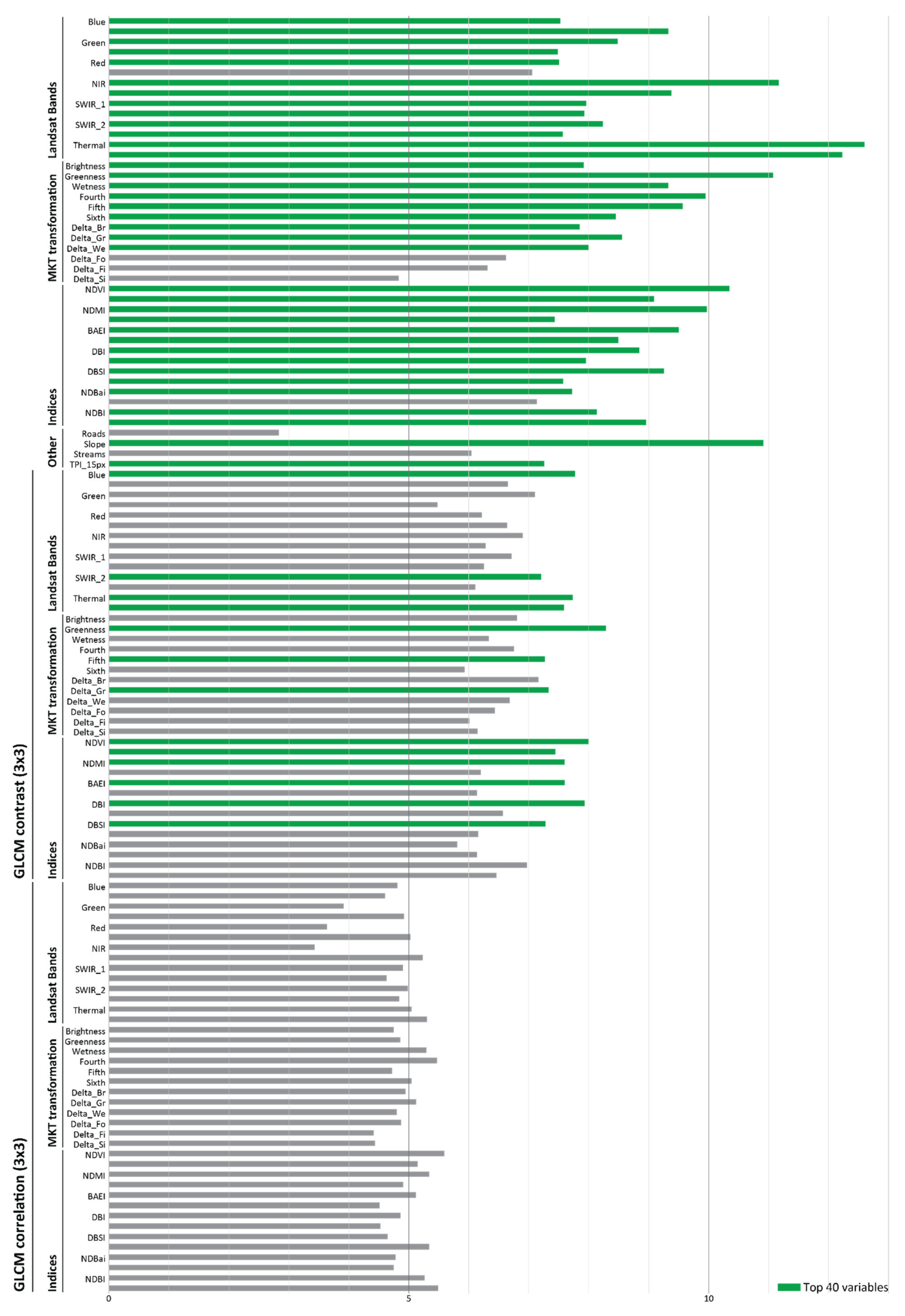
On average across the yearly models, the most important variables for the construction of the RF classifier are Landsat thermal bands for both seasons, MKT greenness, slope, early summer Landsat NIR band, NDMI and NDVI, MKT fifth and fourth components and the BAEI Index for the dry season (Figure 3). While these bands are followed closely in importance by many others which also contribute significantly to the model, they are representative of the different aspects which directly influence LULC in the study area, such as terrain through thermal bands (temperature lowers with elevation) and slope, vegetation (NDVI and NDMI) and its seasonal persistence (greenness), buildings (BAEI), soil (NIR), or a mixture of the above. While elevation is a major driver of vegetation distribution in the study area, we did not use it as a direct input in our models as it tended to overfit the classification over this variable and led to major misclassifications in the agricultural lowlands in the northwestern region of the study area (Figure 1).
The least contributing variable is the mapped roads ancillary data, meaning it is seldom used as a node in the model to differentiate classes, which is consistent with the fact that it mostly aims at discriminating highways (class 21). The 40 least important variables are dominated by GLCM correlation textural features, best used to identify homogeneous patches, which is consistent with the complexity of semi-arid shrublands dominating our study area. However, these variables still contribute significantly to the model, as removing them lead to a drop in the classification’s accuracy. Using more and/or larger texture kernels may increase statistical accuracy of the model, but result in a lower visual performance of the mapped LULC classes as the very frequent isolated houses in the area become undetected.

3.2. Classification Accuracy Assessment

Accuracy assessment is critical to evaluate the quality of a LULC map generated from remote sensing data. The most common way to assess accuracy it is to rely on both visual assessment and on the error matrix of the classification results. In this case, we measured the overall accuracy of each yearly LULC maps using the Kappa statistic, which evaluates the agreement between classification results and reference data after removing the proportion of agreement that could be expected to occur by chance [78]. Kappa values range from −1 (complete disagreement) to 1 (perfect match). In depth analysis of the yearly confusion matrix and derived statistics (overall, user’s and producer’s accuracies) were also used to identify class performances and misclassifications.
The LULC maps generated over the 34 years between 1986 and 2020 (excluding 2012) show good classification results, with overall accuracy (OA) and Kappa (KA) statistics ranging, respectively, from 86.7% and 0.85 in 1986 to 96.3% and 0.96 in 2020 (Supplementary Table S2). While accuracy remains good, classification quality tends to decrease further back in time. The following sections will discuss general trends in the classification results and accuracy statistics for all classes over the entire time period, noting that some variations can occur from year to year.
Water (11), roads (21), evergreen forest (42) and cultivated crops (82) are the most accurately classified classes with >95% producer accuracy (PA) and user accuracy (UA) for every year (but 89.7% PA for cultivated crops in 1986). Grasslands (71), pastures/parks (81) and riparian forests (91) are also well identified, with UA >90% for all years (but 1986), although they only achieve PA > 90% from 1994, 2002, and 1991, respectively. Developed medium and high-density (23 and 24) and barren washes (31) show a similar pattern, but with a lower PA > 80% from 1993, 1996 and 1986, respectively. Shrubs (52) show an opposite pattern, with a generally higher PA (>95%) than UA (>80%) for all years. Developed low-density (22) and barren mines (32) are also relatively well identified, although their performance is a bit lower with UA and PA > 80% (but in early years). Deciduous forests (41) show a decent PA (>80%) but a UA ranging from 60.9 to 84.2%.
The relatively lower classification accuracy of deciduous forests is mostly caused by commission errors over other land covers, notably shrubs, grassland or barren washes, which are often present in the same areas. Such mixed land cover pixels can easily be affected by interannual variations, giving the lead to one or the other LULC classes depending on the climate conditions. Altogether, such shifts between natural vegetation represent 34.5% of pixels misclassifications over the entire time period. Other sources of inaccuracies are confusions within urban land cover classes but with different densities (14.1% of all misclassifications) or with other bright land covers with close spectral signatures, especially barren mines (11.0%) or shrubs (8.5%). Additionally, some isolated houses may remain undetected as they sometimes do not sharply contrast with the shrubland they replace and most buildings are smaller in size than the 30 m Landsat pixel resolution. Confusions between barren mining lands and shrubs (14.2% of misclassifications) can also be noted, inherent to mining cycles with the creation of new tailings and revegetation of older tailings, while our training and validation polygons remained the same over the entire time period.

3.3. Trends in LULC Changes in the Upper Santa Cruz Watershed

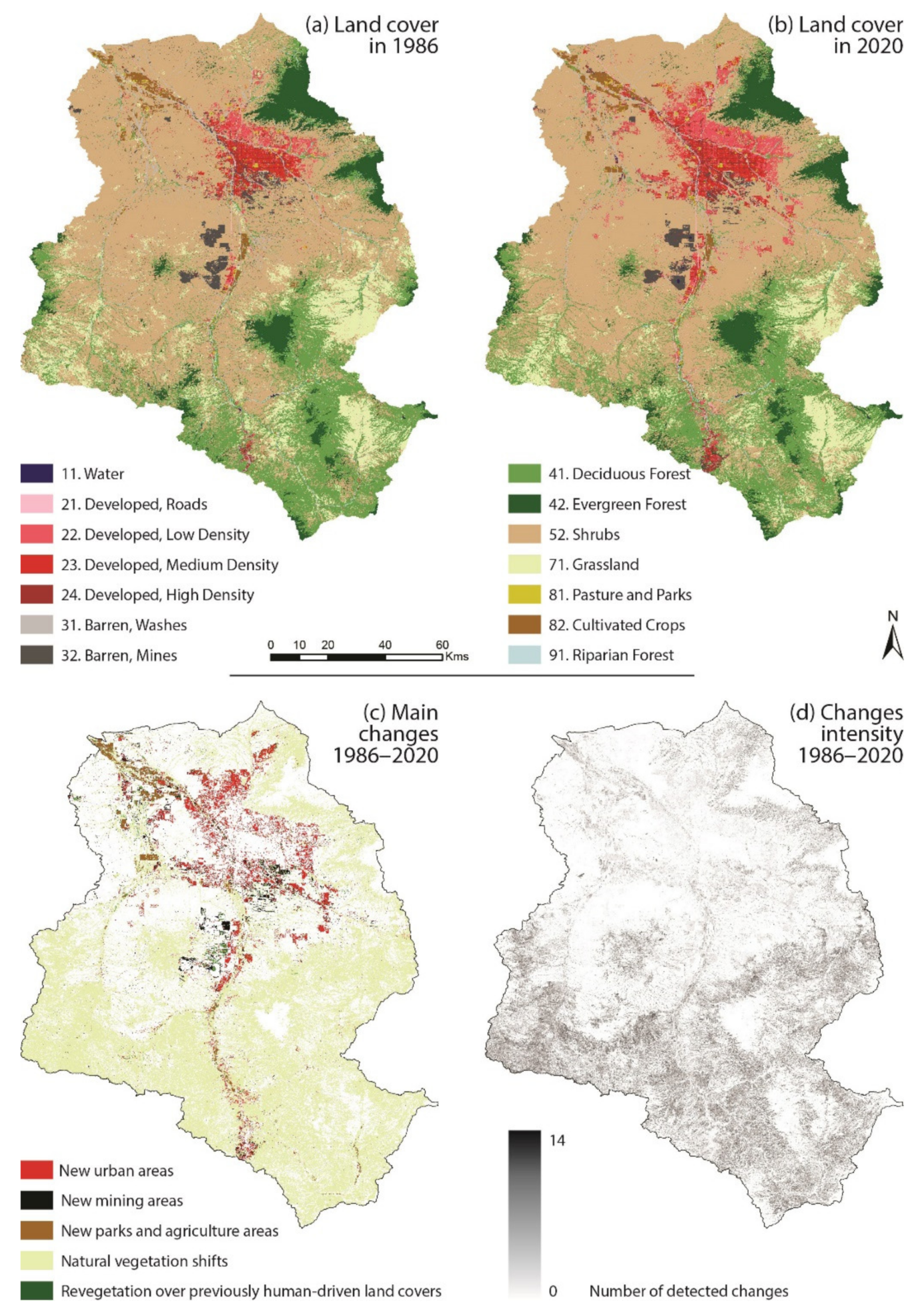
Our yearly classification results provide a clear view of the spatial distribution of LULC types across the study area, from which we can monitor and quantify the important landscape transformations that occurred from 1986 to 2020 (Figure 4 and Supplementary Figure S1). Almost half (48.8%) of the study area witnessed land cover transformations during this time period, most often multiple times (only 9.4% of the region of interest changed only once).
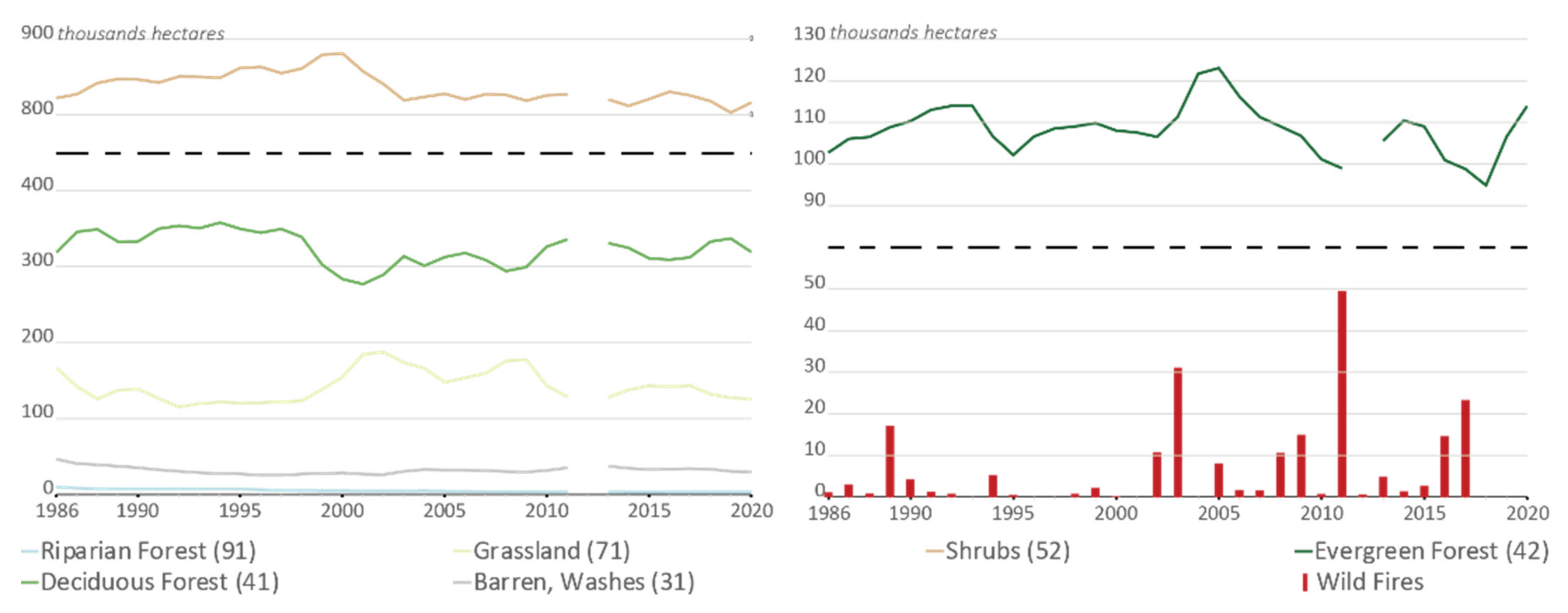
Natural land covers (i.e., shrubs, grasslands, forests and barren washes) are highly dominant in the region, although their share slightly decreases over the 1986–2020 period that we considered, from 92.5% to 88.8% of our overall area of interest (Figure 4). Shifts among natural LULC classes also make up the vast majority of all identified changes (86.8%). Although the respective share of each land cover class can significantly evolve from year to year (Figure 5), natural land covers still maintain a rough balance over the entire time period and at the watershed scale, as most transformations are compensated by opposite trends (Table 3). The most commonly observed dynamics are switches between shrubs and mesquite forests (29.1% of all observed changes), shrubs and grassland (21.1%), deciduous forests and grassland (15.2%), deciduous and evergreen forests (9.6%) and shrubs and evergreen forests (4.6%). These fluctuations can be explained by various factors, notably climatic variations from one year to another as well as prolonged and persistent drought [79,80]. Mesquite encroachment into grasslands is also happening in the south of our study area, but campaigns to mitigate this trend are also in place [81], so that the yearly evolution of their respective total area at the watershed scale appear symmetric (Figure 5). Still, while 27,000 hectares of grassland have been overtaken by mesquite cover, it has only been compensated over 18,000 hectares (about two thirds) by opposite dynamics. While mesquite cover remained constant (albeit fluctuations) at the watershed scale over the 35-year period, grassland cover dropped by 24.5%, mostly replaced by shrublands, which may be a sign of desertification (Figure 5). Evergreen forest covers also show some dramatic decrease which seems to be associated with wildfires [82,83], though forest cover appears to regenerate over the years (Figure 5).
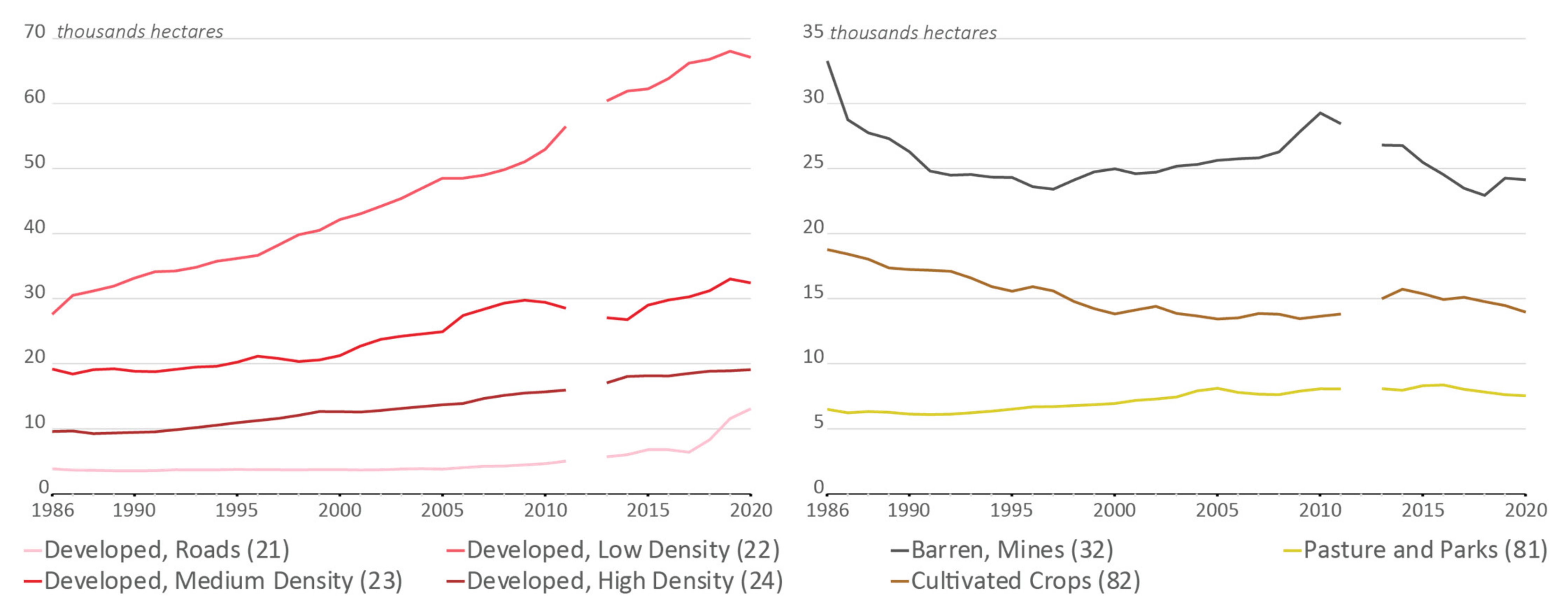
In turn, human-induced land cover changes appear statistically less frequent, as they are most often permanent especially when converting to built-up areas. Such dynamics is the most prominent source of anthropic LULC transformation in the watershed, as newly built urban areas (including roads) account for 2.9% of all observed changes over from 1986 to 2020 (Table 3). Although the area tagged as urban by our model is conservative and thus likely to be an underestimate, it has been steadily increasing in the last three decades and is now largely dominated by low-density residential areas or isolated houses (Figure 4 and Figure 6). Urban development has demonstrated a steady increase and has more than doubled (+118.7%) over the last 35 years (Figure 6). Accommodation of the population immigrating from other parts of the USA to the Tucson metropolitan area is clearly oriented towards building on new lands, mostly shrubs, rather than increasing density in existing urban areas: the expansion rate of low-density urban areas has almost been twice as high as the densification dynamics (+143.2% vs. +79.1%). On average, about 2100 hectares a year have been converted to urban areas since 1986. The urbanization rate has gained steam when the effects of the 2008 crisis did level off, as it increased to 2900 hectares a year after 2010.
The strong pressure this suburbanization puts on the environment in the Tucson region is accompanied by the development of green recreational areas associated with new housing communities. While our pastures and parks class of our model cannot distinguish golf courses from grazing areas due to their very close spectral signature, both are great consumers of water, a scarce resource in the Sonoran Desert. Overall, the total area of the pastures and parks class increased by 16.0% between 1986 and 2020, representing 0.5% of all observed LULC changes across the watershed, replacing mostly shrubs and cultivated crops.
The total area of agriculture over the study area has significantly dropped by 25%, or 4800 hectares, between 1986 and 2020 (Figure 6). Despite this general trend, the replacement of crops by other land covers (mostly shrubs) is highly compensated by the opposite dynamic, accounting, respectively, for 1.2% and 1.0% of all identified changes. While it includes the conversion of never cropped lands to agriculture, this phenomenon is characteristic of the complex rotation of cultures and fallows in irrigated perimeters. According to our LULC classifications, 28% (1350 hectares) of abandoned cultivated lands between 1986 and 2020 have been permanently converted to urban areas, which represent about 7% of the initial cropland cover.
Regarding mining activities, the total area of barren land decreased over the last 35 years (Figure 6). Still, 1.6% of all identified changes over the time period are associated with new mining areas, but which is compensated by the conversion of old tailings (2.0%), mostly revegetated by shrubs. This reflects a slow decrease in mining in the region, where some mines were closed, and no major new pits were open.
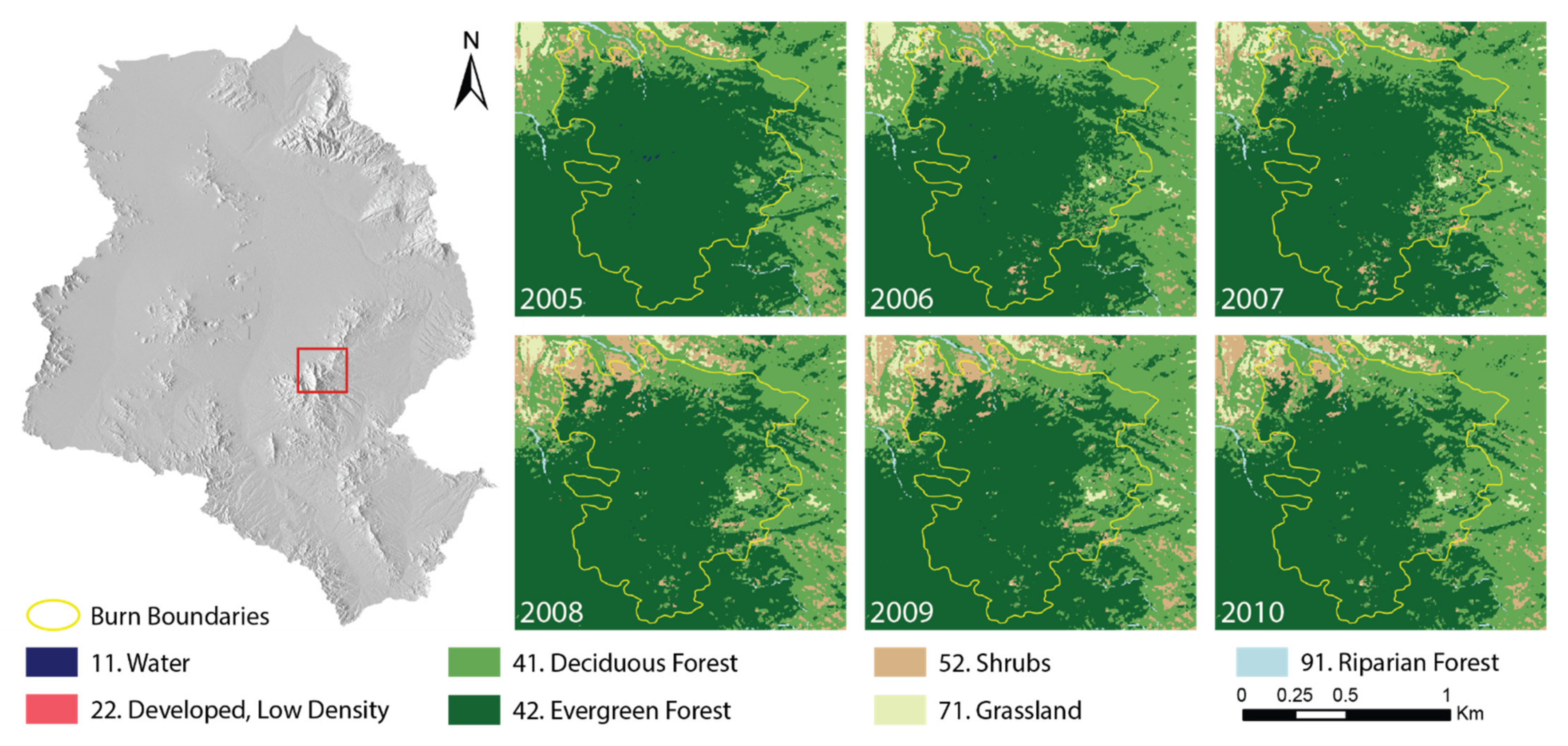
The annual time series of LULC maps resulting from this study allows for the monitoring of spatio-temporal processes that would be difficult to observe using sparser or bi-temporal imagery. The combination of visual and statistical analysis of these maps reflects both sudden transformations of the watershed landscapes, such as the aftereffects of the 2005 Florida wildfire south of Tucson (Figure 5 and Figure 7), or gradual changes spanning several years, such as vegetation regrowth or the spread of built-up areas.

4. Discussion

4.1. Urbanization Patterns in the Upper Santa Cruz Watershed

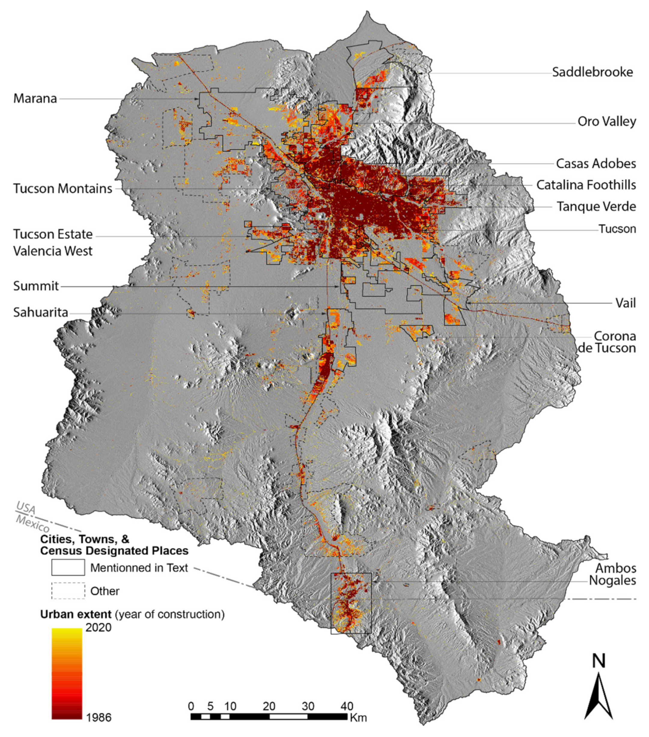
Urban sprawl is a major driver of persistent LULC changes in our study area. To further analyze its spatial distribution, we overlapped our classification results with the legal and statistical entities of United States census designated places [84] while expanding the Ambos Nogales area south to include its Mexican part. This revealed that more than 60% of observed urban sprawl between 1986 and 2020 is located away from cities (Figure 8). Tucson and its directly adjacent statistical areas account for only about a third (34.4%) of the urban extension, mostly in its periphery. While the already significantly developed northern suburbs (Casas Adobes, Catalina Foothills and Tanque Verde) show an urban cover increase of 42.8 to 63.2%, the city is significantly expanding south and west in newly built neighborhoods (Summit, Tucson Estate, Tucson Mountains or Valencia West) where urban cover increased by two to five times its original area in the last 35 years. Nogales was less dynamic, as it only includes 4.0% of the observed urban extension in the watershed.
Already existing small towns have shown massive expansion, such as Oro Valley (+236.8%), Marana (+578.6%) or Sahuarita (+498.9%), located, respectively, north, north-west and south of Tucson, AZ, USA. Altogether, these three towns account for 17.2% of the 1986–2020 urban expansion in the upper Santa Cruz watershed. A number of settlements and recently formed communities have also appeared or are rapidly growing, farther from Tucson while remaining close to the highways, such as Vail in the east (+1251.5%), Saddlebrooke in the north (+1196.4%) or Corona de Tucson in the south (+1106.3%). While these are now significant enough to be included in census designated places, it has to be noted that 20.6% of all urban expansion observed by our study happens away from all statistical areas, composed mostly of isolated houses or newly built communities.
Such leapfrog urbanization is not new in the region and is putting an increasing pressure on a fragile ecosystem with scarce resources [85,86]. Water is the main concern, since the region is arid. Heavy groundwater pumping led to a declining water table in the 1990s, when plans and legislative acts reorganized some of the withdrawal of groundwater resources and provided a new supply through the Central Arizona Project Canal [87,88,89]. Even if the average consumption of water by person dropped significantly in cities [5], availability is still a concern in the face of climate change and continuing expansion of urban areas [12], although the Arizona Groundwater Management Act of 1980 requires developers to prove access to a one-hundred-year water supply in order to tackle this issue.
Habitat fragmentation of the typical open-space landscape of the Sonoran Desert is also a concern. The Pima County, which has been sensible to environmental preservation as early as the 1930s [90], adopted in response its Sonoran Desert Conservation Plan in 1999 and subsequently made attempts to purchase ranchland to slow the conversion of agricultural land to urban use [91] and maintain “open spaces”. While protected areas have mostly been preserved from new settlements, such political interventions have not significantly changed the model of urban growth around Tucson in the last decade.

4.2. Main Drivers of Inaccuracies in Our Yearly Classifications

As noted before, inaccuracies in our model are strongly correlated with time, LULC classification being less performant as we go back in past years. This is most likely due to the fact that we favored an automated process over the entire 1986–2020 period, thus using the same training and validation polygons for the entire time series. While high-resolution satellite imagery can be used as “ground truth” in recent years, available aerial imagery in the 1970s and 1980s is scarcer and of much coarser resolution. Our training and validation datasets are less accurate back then, as they may contain uncorrected errors for the LULC classes they actually cover on the ground at these times.
While Landsat data provide opportunities for consistent time series of satellite imageries spanning several decades, its medium-high resolution of 30 m can complicate the identification of smaller targets, such as the isolated houses characteristic of some urbanization dynamics in the Tucson area. This issue is compensated to some extent by the use of 3 × 3 pixel GLCM texture kernels allowing for the better detection of spatial variations in the spectral signature of pixels that may include single houses (i.e., bright built-up areas surrounded by green vegetation). As a result, our yearly classifications are highly sensitive to such patterns, with a good detection of low-density urban areas, at the cost of some commission errors in other bright areas of heterogeneous composition, such as washes or mine tailings.
One of the solutions used to mitigate these trends was to use our conservative routine on urban pixels. It is based on the hypothesis that urban extent is expanding in the area, so that built-up areas are unlikely to revert back to other LULC classes, and thus corrects any pixel identified as urban for one year and non-urban for later years. This allowed us to greatly reduce their occurrence and to gain significant visual accuracy, while statistical accuracy (Kappa and OA) remained roughly the same on average over the yearly classification results. We were thus able to better identify urbanization dynamics. However, while our model had the tendency to mix up dense urban pixels and barren mining lands in its detection capacities, this routine had the side effect to lower its ability to detect some types of urban areas. In the south of Nogales, for instance, some dense urban areas are mapped as barren mining areas, probably because of the type of construction material and geometry of urbanization in Mexico, which differs from urban and suburban areas in the United States, where most of our training samples are located.
Still, we should also underline that a major source of inaccuracies in our model is happening between classes of natural vegetation (34.5% between 1986 and 2020) or within different urban classes (14.1%). For example, mesquite trees (class 41) are often misidentified over arroyos, herbaceous cover and riverine or evergreen forests, mainly in areas presenting a mixture of these different land covers. Thus, these can be considered “relative” errors rather than “absolute” errors, as they related to the proportional share of these mixed land covers within a pixel, which can also change over the years while our training and validation polygons remain the same. While shrubs (class 52) may be mapped over barren mine pits (due to their revegetation) and low-density urban areas, they may also be mapped over other low-vegetation classes, such as drying-up grassland and pastures. These misclassifications may be related to climate variations across the years, disregarded by our static training and validation data. To corroborate this assumption, we already noted that LULC changes over the analyzed period are highly dominated by shifts within natural vegetation classes (see Figure 4c,d). This can also be caused by slight variations of the land cover within mixed pixels, thus leading to biased estimates of land cover transformations in the watershed. Hence, integrating sub-pixel analysis [92,93,94] may be useful to overcome the impact of mixed pixels in yearly classification inaccuracies and derived change analysis.

4.3. Paths for Expanding and Improving the Model

The yearly LULC classifications we have produced between 1986 and 2020 rely primarily on Landsat 5 and Landsat 8 images. The code which was elaborated can already process all forthcoming years as long as Landsat 8 and now Landsat 9 continue to operate and could be adapted to also process other data sources in the future, such as Sentinel-2 imagery. For now, as the current year is used in post-processing, only LULC maps of the preceding year can be computed (if imagery is available for both needed seasons in a year to compute MKT transformations, which is by the end of November). However, if the 35-year period covered in this study can be expanded towards future years, expanding it in the past could also be interesting in order to better document the history of urban growth and environmental change in the area.
Such an extension backwards in time is, however, a complex task. In effect, our study is based on the use of pre-processed Tier 1 Landsat SR products, which are less readily available before 1986. We could extend the coverage of our analysis to July 1982 and the launch of Landsat 4 TM, but this would require a custom raw data pre-processing which could lead in incompatibility with further data. Additionally, the use of Landsat MSS data would be necessary to go back farther than 1982, but those images are not available as SR products, and both spectral bands and resolution are not really the same as Landsat TM, so consistency over the classification process and results are not guaranteed when using these. Use of MSS would potentially allow one to go back as far as 1972, but it is to be expected that accuracy will be much lower, also because image availability and quality would be lower than for MSS, leading to more misclassified pixels for each year.
One way to further improve the accuracy of our model would be to manually refine our training and validation datasets, as well as Landsat scene selection, for each year. So far, we accepted images with a rather high cloud cover, and we selected rather large time windows for each of the two seasons we considered. This was necessary in order to not have too many NoData pixels—i.e., areas masked out by our image pre-processing technique removing clouds, cloud edges and saturated pixels. Raw image quality or season-specific spectral signature detection might be improved by manually picking Landsat scenes and thus lowering both these filters, but without the confidence to gain full coverage images for each year. However, this would drastically increase human intervention while we favored an automated process which allows us to rapidly process long time series. Moreover, selecting images manually with different characteristics and editing training and validation data for each year would make the whole methodology more time consuming, with the additional cost of being less reproducible over the entire time series.
Lastly, as one goal of this research is to provide a generic and adaptative GEE script for computing annual LULC time series over different regions of interests, the robustness of our method shall be tested not only in comparable areas with similar issues (such as the US Southwest as a whole), but also beyond desert landscapes with adjusted land cover indicators.

5. Conclusions

We propose in this study an automated multi-temporal and multi-sensor classification method to extract yearly LULC data for the Tucson area since the mid-80s. Hosting the entire workflow in the GEE platform allowed us to quickly process very large datasets and to maintain a consistent methodology for the entire 1986–2020 period and on to oncoming years. We used a number of post-processing techniques to mitigate inevitable issues in temporal LULC change monitoring, such as smoothing the influence of interannual climate variations or addressing possible misclassifications associated with the lack of availability of robust ground truth imagery to build our model training datasets as we go further back in time. For most years, we achieved very satisfying classification accuracy (over 90 to 95%), allowing us to monitor landscape transformations in southern Arizona from then and in the future. While this analysis focused on the production of a long time series of annual LULC maps, future lines of research shall focus on detected change verification, as well as identification of their mechanisms and their driving forces (e.g., climate change or land use policies) in the upper Santa Cruz watershed.
Our methodology demonstrates the potential of the enormous cloud calculation capabilities offered by GEE. This server-sided technology allowed us to not only save a considerable amount of time in comparison with the traditional desktop computing techniques, but also assures our scripts are adaptable for any other project with similar needs over different regions of interest, in order to provide critical and timely information with high temporal depth to decision makers.

Supplementary Materials

The following supporting information can be downloaded at: https://www.mdpi.com/article/10.3390/rs14092127/s1, Figure S1: Maps of yearly land cover classification results (1986–2020); Table S1: Training/validation dataset composition; Table S2: Confusion matrix for years 1986–2020.

Author Contributions

Conceptualization, F.D., F.-M.L.T. and M.L.V.; methodology, F.D.; software, F.D.; validation, F.D. and F.-M.L.T.; formal analysis, F.D. and F.-M.L.T.; investigation, F.D. and F.-M.L.T.; resources, F.D. and M.L.V.; data curation, F.D.; writing—original draft preparation, F.D.; writing—review and editing, F.D., F.-M.L.T., M.L.V. and L.M.N.; visualization, F.D.; supervision, F.-M.L.T.; project administration, F.D. and F.-M.L.T.; funding acquisition, F.-M.L.T. All authors have read and agreed to the published version of the manuscript.

Funding

This research was funded by a grant from the LabEx DRIHM, French Programme “Investissements d’Avenir” (ANR-11-LABX-0010), which is managed by the French National Research Agency (Agence Nationale de la Recherche, or ANR). M.L.V. and L.M.N. are supported by the Land Change Science Program of the U.S. Geological Survey.

Data Availability Statement

The yearly LULC classification results, the GEE scripts and other ancillary data supporting this study are open access; See Dubertret, F., Le Tourneau, F.M., Villarreal, M.L. and L.M. Norman. 2022. Annual (1986–2020) land-use/land cover maps of the Tucson metropolitan area, Arizona: U.S. Geological Survey data release, https://doi.org/10.5066/P9XC5Y36 (accessed on 14 April 2022).

Acknowledgments

We would like to thank the four anonymous reviewers, as well as Roy E. Petrakis and Geneva W. Chong for their comments and suggestions on how to further improve the first drafts of this article. Any use of trade, firm or product names is for descriptive purposes only and does not imply endorsement by the U.S. Government.

Conflicts of Interest

The authors declare no conflict of interest.

References

  1. Sheridan, T.E. Arizona: A History, Rev. ed.; Southwest Center Series; University of Arizona Press: Tucson, AZ, USA, 2012; ISBN 978-0-8165-0687-3. [Google Scholar]
  2. Devine, D. Tucson: A History of the Old Pueblo from the 1854 Gadsden Purchase; McFarland & Company, Inc.: Jefferson, NC, USA, 2015; ISBN 978-0-7864-9710-2. [Google Scholar]
  3. Norman, L.M.; Feller, M.; Villarreal, M.L. Developing Spatially Explicit Footprints of Plausible Land-Use Scenarios in the Santa Cruz Watershed, Arizona and Sonora. Landsc. Urban Plan. 2012, 107, 225–235. [Google Scholar] [CrossRef] [Green Version]
  4. U.S. Census Bureau. 2020 Census Results. Available online: https://data.census.gov/ (accessed on 14 April 2022).
  5. Le Tourneau, F.-M.; Dubertret, F. Space and water, key factors of urban growth in the South-Western United States: Case study of Tucson and Pima County (Arizona). Espace Géographique 2019, 48, 39–56. [Google Scholar] [CrossRef]
  6. Sheridan, T.E. Cows, Condos, and the Contested Commons: The Political Ecology of Ranching on the Arizona-Sonora Borderlands. Hum. Organ. 2001, 60, 141–152. [Google Scholar] [CrossRef]
  7. Vukomanovic, J.; Vogler, J.B.; Petrasova, A. Modeling the Connection between Viewscapes and Home Locations in a Rapidly Exurbanizing Region. Comput. Environ. Urban Syst. 2019, 78, 101388. [Google Scholar] [CrossRef]
  8. Niraula, R.; Meixner, T.; Norman, L.M. Determining the Importance of Model Calibration for Forecasting Absolute/Relative Changes in Streamflow from LULC and Climate Changes. J. Hydrol. 2015, 522, 439–451. [Google Scholar] [CrossRef]
  9. Norman, L.; Tallent-Halsell, N.; Labiosa, W.; Weber, M.; McCoy, A.; Hirschboeck, K.; Callegary, J.; Van Riper, C.; Gray, F. Developing an Ecosystem Services Online Decision Support Tool to Assess the Impacts of Climate Change and Urban Growth in the Santa Cruz Watershed; Where We Live, Work, and Play. Sustainability 2010, 2, 2044–2069. [Google Scholar] [CrossRef] [Green Version]
  10. Villarreal, M.L.; Norman, L.M.; Boykin, K.G.; Wallace, C.S.A. Biodiversity Losses and Conservation Trade-Offs: Assessing Future Urban Growth Scenarios for a North American Trade Corridor. Int. J. Biodivers. Sci. Ecosyst. Serv. Manag. 2013, 9, 90–103. [Google Scholar] [CrossRef]
  11. Norman, L.M.; Villarreal, M.L.; Lara-Valencia, F.; Yuan, Y.; Nie, W.; Wilson, S.; Amaya, G.; Sleeter, R. Mapping Socio-Environmentally Vulnerable Populations Access and Exposure to Ecosystem Services at the U.S.–Mexico Borderlands. Appl. Geogr. 2012, 34, 413–424. [Google Scholar] [CrossRef]
  12. Yang, Z.; Dominguez, F.; Gupta, H.; Zeng, X.; Norman, L. Urban Effects on Regional Climate: A Case Study in the Phoenix and Tucson “Sun Corridor”. Earth Interact. 2016, 20, 1–25. [Google Scholar] [CrossRef]
  13. Garfin, G.; Jardine, A.; Merideth, R.; Black, M.; LeRoy, S. Assessment of Climate Change in the Southwest United States: A Report Prepared for the National Climate Assessment; A report by the Southwest Climate Alliance; Island Press: Washington, DC, USA, 2013. [Google Scholar]
  14. Gonzalez, P.; Garfin, G.M.; Breshears, D.; Brooks, K.; Brown, H.E.; Elias, E.; Gunasekara, A.; Huntly, N.; Maldonado, J.K.; Mantua, N.J.; et al. Chapter 25: Southwest. In Impacts, Risks, and Adaptation in the United States: The Fourth National Climate Assessment, Volume II; Reidmiller, D.R., Avery, C.W., Easterling, D.R., Kunkel, K.E., Lewis, K.L.M., Maycock, T.K., Stewart, B.C., Eds.; U.S. Global Change Research Program: Washington, DC, USA, 2018; pp. 1101–1184. [Google Scholar] [CrossRef]
  15. Ghasemi Tousi, E.; O’Brien, W.; Doulabian, S.; Shadmehri Toosi, A. Climate Changes Impact on Stormwater Infrastructure Design in Tucson Arizona. Sustain. Cities Soc. 2021, 72, 103014. [Google Scholar] [CrossRef]
  16. Latifovic, R.; Homer, C.; Ressl, R.; Pouliot, D.A.; Hossian, S.; Colditz, R.; Olthof, I.; Chandra, G.; Victoria, A. North American Land Change Monitoring System. In Remote Sensing of Land Use and Land Cover: Principles and Applications; Giri, C.P., Ed.; CRC Press: Boca Raton, FL, USA, 2012; pp. 303–324. [Google Scholar] [CrossRef]
  17. Brown, J.F.; Tollerud, H.J.; Barber, C.P.; Zhou, Q.; Dwyer, J.L.; Vogelmann, J.E.; Loveland, T.R.; Woodcock, C.E.; Stehman, S.V.; Zhu, Z.; et al. Lessons Learned Implementing an Operational Continuous United States National Land Change Monitoring Capability: The Land Change Monitoring, Assessment, and Projection (LCMAP) Approach. Remote Sens. Environ. 2020, 238, 111356. [Google Scholar] [CrossRef]
  18. Auch, R.F.; Wellington, D.F.; Taylor, J.L.; Stehman, S.V.; Tollerud, H.J.; Brown, J.F.; Loveland, T.R.; Pengra, B.W.; Horton, J.A.; Zhu, Z.; et al. Conterminous United States Land-Cover Change (1985–2016): New Insights from Annual Time Series. Land 2022, 11, 298. [Google Scholar] [CrossRef]
  19. Villarreal, M.; Norman, L.; Wallace, C.; van Riper, C. A Multitemporal (1979–2009) Land-Use/Land-Cover Dataset of the Binational Santa Cruz Watershed. In Open-File Report 2011–1131; U.S. Geological Survey: Reston, VA, USA, 2011; p. 26. [Google Scholar]
  20. Wickham, J.; Homer, C.; Vogelmann, J.; McKerrow, A.; Mueller, R.; Herold, N.; Coulston, J. The Multi-Resolution Land Characteristics (MRLC) Consortium—20 Years of Development and Integration of USA National Land Cover Data. Remote Sens. 2014, 6, 7424–7441. [Google Scholar] [CrossRef] [Green Version]
  21. Hansen, M.C.; Egorov, A.; Potapov, P.V.; Stehman, S.V.; Tyukavina, A.; Turubanova, S.A.; Roy, D.P.; Goetz, S.J.; Loveland, T.R.; Ju, J.; et al. Monitoring Conterminous United States (CONUS) Land Cover Change with Web-Enabled Landsat Data (WELD). Remote Sens. Environ. 2014, 140, 466–484. [Google Scholar] [CrossRef] [Green Version]
  22. Homer, C.; Dewitz, J.; Jin, S.; Xian, G.; Costello, C.; Danielson, P.; Gass, L.; Funk, M.; Wickham, J.; Stehman, S.; et al. Conterminous United States Land Cover Change Patterns 2001–2016 from the 2016 National Land Cover Database. ISPRS J. Photogramm. Remote Sens. 2020, 162, 184–199. [Google Scholar] [CrossRef]
  23. Li, X.; Zhou, Y.; Zhu, Z.; Cao, W. A National Dataset of 30 m Annual Urban Extent Dynamics (1985–2015) in the Conterminous United States. Earth Syst. Sci. Data 2020, 12, 357–371. [Google Scholar] [CrossRef] [Green Version]
  24. Lark, T.J.; Mueller, R.M.; Johnson, D.M.; Gibbs, H.K. Measuring Land-Use and Land-Cover Change Using the U.S. Department of Agriculture’s Cropland Data Layer: Cautions and Recommendations. Int. J. Appl. Earth Obs. Geoinf. 2017, 62, 224–235. [Google Scholar] [CrossRef]
  25. Farahani, M.; Mohammadzadeh, A. Domain Adaptation for Unsupervised Change Detection of Multisensor Multitemporal Remote-Sensing Images. Int. J. Remote Sens. 2020, 41, 3902–3923. [Google Scholar] [CrossRef]
  26. Phan, T.N.; Kuch, V.; Lehnert, L.W. Land Cover Classification Using Google Earth Engine and Random Forest Classifier—The Role of Image Composition. Remote Sens. 2020, 12, 2411. [Google Scholar] [CrossRef]
  27. Casu, F.; Manunta, M.; Agram, P.S.; Crippen, R.E. Big Remotely Sensed Data: Tools, Applications and Experiences. Remote Sens. Environ. 2017, 202, 1–2. [Google Scholar] [CrossRef]
  28. Gorelick, N.; Hancher, M.; Dixon, M.; Ilyushchenko, S.; Thau, D.; Moore, R. Google Earth Engine: Planetary-Scale Geospatial Analysis for Everyone. Remote Sens. Environ. 2017, 202, 18–27. [Google Scholar] [CrossRef]
  29. Huang, H.; Chen, W.; Zhang, Y.; Qiao, L.; Du, Y. Analysis of Ecological Quality in Lhasa Metropolitan Area during 1990–2017 Based on Remote Sensing and Google Earth Engine Platform. J. Geogr. Sci. 2021, 31, 265–280. [Google Scholar] [CrossRef]
  30. Xie, S.; Liu, L.; Zhang, X.; Yang, J.; Chen, X.; Gao, Y. Automatic Land-Cover Mapping Using Landsat Time-Series Data Based on Google Earth Engine. Remote Sens. 2019, 11, 3023. [Google Scholar] [CrossRef] [Green Version]
  31. Wulder, M.A.; Coops, N.C.; Roy, D.P.; White, J.C.; Hermosilla, T. Land Cover 2.0. Int. J. Remote Sens. 2018, 39, 4254–4284. [Google Scholar] [CrossRef] [Green Version]
  32. Xu, J.; Xiao, W.; He, T.; Deng, X.; Chen, W. Extraction of Built-up Area Using Multi-Sensor Data—A Case Study Based on Google Earth Engine in Zhejiang Province, China. Int. J. Remote Sens. 2021, 42, 389–404. [Google Scholar] [CrossRef]
  33. Souza, C.M., Jr.; Shimbo, J.Z.; Rosa, M.R.; Parente, L.L.; Alencar, A.A.; Rudorff, B.F.T.; Hasenack, H.; Matsumoto, M.; Ferreira, L.G.; Souza-Filho, P.W.M.; et al. Reconstructing Three Decades of Land Use and Land Cover Changes in Brazilian Biomes with Landsat Archive and Earth Engine. Remote Sens. 2020, 12, 2735. [Google Scholar] [CrossRef]
  34. Xia, H.; Zhao, J.; Qin, Y.; Yang, J.; Cui, Y.; Song, H.; Ma, L.; Jin, N.; Meng, Q. Changes in Water Surface Area during 1989–2017 in the Huai River Basin Using Landsat Data and Google Earth Engine. Remote Sens. 2019, 11, 1824. [Google Scholar] [CrossRef] [Green Version]
  35. Kumar, L.; Mutanga, O. Google Earth Engine Applications Since Inception: Usage, Trends, and Potential. Remote Sens. 2018, 10, 1509. [Google Scholar] [CrossRef] [Green Version]
  36. Wang, L.; Diao, C.; Xian, G.; Yin, D.; Lu, Y.; Zou, S.; Erickson, T.A. A Summary of the Special Issue on Remote Sensing of Land Change Science with Google Earth Engine. Remote Sens. Environ. 2020, 248, 112002. [Google Scholar] [CrossRef]
  37. Liu, X.; Hu, G.; Chen, Y.; Li, X.; Xu, X.; Li, S.; Pei, F.; Wang, S. High-Resolution Multi-Temporal Mapping of Global Urban Land Using Landsat Images Based on the Google Earth Engine Platform. Remote Sens. Environ. 2018, 209, 227–239. [Google Scholar] [CrossRef]
  38. Zhang, X.; Liu, L.; Wu, C.; Chen, X.; Gao, Y.; Xie, S.; Zhang, B. Development of a Global 30 m Impervious Surface Map Using Multisource and Multitemporal Remote Sensing Datasets with the Google Earth Engine Platform. Earth Syst. Sci. Data 2020, 12, 1625–1648. [Google Scholar] [CrossRef]
  39. Tang, Z.; Li, Y.; Gu, Y.; Jiang, W.; Xue, Y.; Hu, Q.; LaGrange, T.; Bishop, A.; Drahota, J.; Li, R. Assessing Nebraska Playa Wetland Inundation Status during 1985–2015 Using Landsat Data and Google Earth Engine. Environ. Monit. Assess. 2016, 188, 654. [Google Scholar] [CrossRef] [PubMed]
  40. Floreano, I.X.; de Moraes, L.A.F. Land Use/Land Cover (LULC) Analysis (2009–2019) with Google Earth Engine and 2030 Prediction Using Markov-CA in the Rondônia State, Brazil. Environ. Monit. Assess. 2021, 193, 239. [Google Scholar] [CrossRef]
  41. Nechyba, T.J.; Walsh, R.P. Urban Sprawl. J. Econ. Perspect. 2004, 18, 177–200. [Google Scholar] [CrossRef] [Green Version]
  42. Dubertret, F.; Le Tourneau, F.-M.; Villareal, M.; Norman, L. Annual (1986–2020) Land-Use/Land Cover Maps of the Tucson Metropolitan Area, Arizona. U.S. Geological Survey. 2022. Available online: https://www.sciencebase.gov/catalog/item/61fc4f6cd34e622189cbd903 (accessed on 14 April 2022).
  43. Farr, T.G.; Rosen, P.A.; Caro, E.; Crippen, R.; Duren, R.; Hensley, S.; Kobrick, M.; Paller, M.; Rodriguez, E.; Roth, L.; et al. The Shuttle Radar Topography Mission. Rev. Geophys. 2007, 45, RG2004. [Google Scholar] [CrossRef] [Green Version]
  44. U.S. Geological Survey. USGS National Hydrography Dataset Plus High Resolution (NHDPlus HR) for 4-Digit Hydrologic Unit-1505 (Published 20180813). Available online: https://www.sciencebase.gov/catalog/item/5d30c292e4b01d82ce84aa32 (accessed on 14 April 2022).
  45. Global Administrative Areas Digital Geospatial Data. University of California, Berkeley, Museum of Vertebrate Zoology and the International Rice Research Institute. Available online: http://www.gadm.org/ (accessed on 14 April 2022).
  46. Wallace, C.; Villarreal, M.; Norman, L. Development of a High-Resolution Binational Vegetation Map of the Santa Cruz River Riparian Corridor and Surrounding Watershed, Southern Arizona and Northern Sonora, Mexico. In Open-File Report 2011-1143; U.S. Geological Survey: Reston, VA, USA, 2011; p. 22. [Google Scholar] [CrossRef]
  47. Norman, L.; Donelson, A.; Pfeifer, E.; Lam, A. Colonia Development and Land Use Change in Ambos Nogales, United States-Mexican Border. In Open-File Report 2006-1112; U.S. Geological Survey: Reston, VA, USA, 2006; p. 121. [Google Scholar] [CrossRef]
  48. Norman, L.M.; Wallace, C.S.A. Mapping Land Use/Land Cover in the Ambos Nogales Study Area. In Open-File Report 2008-1378; U.S. Geological Survey: Reston, VA, USA, 2008. [Google Scholar] [CrossRef]
  49. Foga, S.; Scaramuzza, P.L.; Guo, S.; Zhu, Z.; Dilley, R.D.; Beckmann, T.; Schmidt, G.L.; Dwyer, J.L.; Joseph Hughes, M.; Laue, B. Cloud Detection Algorithm Comparison and Validation for Operational Landsat Data Products. Remote Sens. Environ. 2017, 194, 379–390. [Google Scholar] [CrossRef] [Green Version]
  50. Hagolle, O.; Colin, J. Several Issues Found in Recent Papers on Cloud Detection Published in MDPI Remote Sensing. Available online: https://labo.obs-mip.fr/multitemp/issues-with-mdpi-remote-sensing-recent-papers-on-cloud-detection/ (accessed on 14 April 2022).
  51. Roy, D.P.; Zhang, H.K.; Ju, J.; Gomez-Dans, J.L.; Lewis, P.E.; Schaaf, C.B.; Sun, Q.; Li, J.; Huang, H.; Kovalskyy, V. A General Method to Normalize Landsat Reflectance Data to Nadir BRDF Adjusted Reflectance. Remote Sens. Environ. 2016, 176, 255–271. [Google Scholar] [CrossRef] [Green Version]
  52. Soenen, S.A.; Peddle, D.R.; Coburn, C.A. SCS + C: A Modified Sun-Canopy-Sensor Topographic Correction in Forested Terrain. IEEE Trans. Geosci. Remote Sens. 2005, 43, 2148–2159. [Google Scholar] [CrossRef]
  53. Dong, C.; Zhao, G.; Meng, Y.; Li, B.; Peng, B. The Effect of Topographic Correction on Forest Tree Species Classification Accuracy. Remote Sens. 2020, 12, 787. [Google Scholar] [CrossRef] [Green Version]
  54. Fang, Y.; Zhao, J.; Liu, L.; Wang, J. Comparision of Eight Topographic Correction Algorithms Applied to Landsat-8 OLI Imagery Based on the DEM. IOP Conf. Ser. Earth Environ. Sci. 2020, 428, 012051. [Google Scholar] [CrossRef] [Green Version]
  55. Vázquez-Jiménez, R.; Romero-Calcerrada, R.; Ramos-Bernal, R.; Arrogante-Funes, P.; Novillo, C. Topographic Correction to Landsat Imagery through Slope Classification by Applying the SCS + C Method in Mountainous Forest Areas. ISPRS Int. J. Geo-Inf. 2017, 6, 287. [Google Scholar] [CrossRef]
  56. Tucker, C.J. Red and Photographic Infrared Linear Combinations for Monitoring Vegetation. Remote Sens. Environ. 1979, 8, 127–150. [Google Scholar] [CrossRef] [Green Version]
  57. Gao, B. NDWI—A Normalized Difference Water Index for Remote Sensing of Vegetation Liquid Water from Space. Remote Sens. Environ. 1996, 58, 257–266. [Google Scholar] [CrossRef]
  58. Bramhe, V.S.; Ghosh, S.K.; Garg, P.K. Extraction of Built-Up Area by Combining Textural Features and Spectral Indices from LANDSAT-8 Multispectral Image. ISPRS-Int. Arch. Photogramm. Remote Sens. Spat. Inf. Sci. 2018, 425, 727–733. [Google Scholar] [CrossRef] [Green Version]
  59. Rasul, A.; Balzter, H.; Ibrahim, G.R.F.; Hameed, H.M.; Wheeler, J.; Adamu, B.; Ibrahim, S.; Najmaddin, P.M. Applying Built-Up and Bare-Soil Indices from Landsat 8 to Cities in Dry Climates. Land 2018, 7, 81. [Google Scholar] [CrossRef] [Green Version]
  60. Guisan, A.; Weiss, S.B.; Weiss, A.D. GLM versus CCA Spatial Modeling of Plant Species Distribution. Plant Ecol. 1999, 143, 107–122. [Google Scholar] [CrossRef]
  61. Weiss, A.D. Topographic Position and Landforms Analysis. In Proceedings of the ESRI User Conference, San Diego, CA, USA, 9–13 July 2001. [Google Scholar]
  62. De Reu, J.; Bourgeois, J.; Bats, M.; Zwertvaegher, A.; Gelorini, V.; De Smedt, P.; Chu, W.; Antrop, M.; De Maeyer, P.; Finke, P.; et al. Application of the Topographic Position Index to Heterogeneous Landscapes. Geomorphology 2013, 186, 39–49. [Google Scholar] [CrossRef]
  63. Hall-Beyer, M. Practical Guidelines for Choosing GLCM Textures to Use in Landscape Classification Tasks over a Range of Moderate Spatial Scales. Int. J. Remote Sens. 2017, 38, 1312–1338. [Google Scholar] [CrossRef]
  64. Collins, J.B.; Woodcock, C.E. An Assessment of Several Linear Change Detection Techniques for Mapping Forest Mortality Using Multitemporal Landsat TM Data. Remote Sens. Environ. 1996, 56, 66–77. [Google Scholar] [CrossRef]
  65. Baig, M.H.A.; Zhang, L.; Shuai, T.; Tong, Q. Derivation of a Tasselled Cap Transformation Based on Landsat 8 At-Satellite Reflectance. Remote Sens. Lett. 2014, 5, 423–431. [Google Scholar] [CrossRef]
  66. Sonobe, R.; Yamaya, Y.; Tani, H.; Wang, X.; Kobayashi, N.; Mochizuki, K. Mapping Crop Cover Using Multi-Temporal Landsat 8 OLI Imagery. Int. J. Remote Sens. 2017, 38, 4348–4361. [Google Scholar] [CrossRef] [Green Version]
  67. OSM Contributors Planet Dump [Data File from 2021/04/12]. Available online: https://planet.openstreetmap.org (accessed on 14 April 2022).
  68. Homer, C.; Dewitz, J.; Yang, L.; Jin, S.; Danielson, P.; Xian, G.; Coulston, J.; Herold, N.; Wickham, J.; Megown, K. Completion of the 2011 National Land Cover Database for the Conterminous United States—Representing a Decade of Land Cover Change Information. Photogramm. Eng. Remote Sens. 2015, 81, 346–354. [Google Scholar] [CrossRef]
  69. Yang, L.; Jin, S.; Danielson, P.; Homer, C.; Gass, L.; Bender, S.M.; Case, A.; Costello, C.; Dewitz, J.; Fry, J.; et al. A New Generation of the United States National Land Cover Database: Requirements, Research Priorities, Design, and Implementation Strategies. ISPRS J. Photogramm. Remote Sens. 2018, 146, 108–123. [Google Scholar] [CrossRef]
  70. Pal, M. Random Forest Classifier for Remote Sensing Classification. Int. J. Remote Sens. 2005, 26, 217–222. [Google Scholar] [CrossRef]
  71. Gislason, P.O.; Benediktsson, J.A.; Sveinsson, J.R. Random Forests for Land Cover Classification. Pattern Recognit. Lett. 2006, 27, 294–300. [Google Scholar] [CrossRef]
  72. Rodriguez-Galiano, V.F.; Ghimire, B.; Rogan, J.; Chica-Olmo, M.; Rigol-Sanchez, J.P. An Assessment of the Effectiveness of a Random Forest Classifier for Land-Cover Classification. ISPRS J. Photogramm. Remote Sens. 2012, 67, 93–104. [Google Scholar] [CrossRef]
  73. Thanh Noi, P.; Kappas, M. Comparison of Random Forest, k-Nearest Neighbor, and Support Vector Machine Classifiers for Land Cover Classification Using Sentinel-2 Imagery. Sensors 2017, 18, 18. [Google Scholar] [CrossRef] [Green Version]
  74. Ho, T.K. The Random Subspace Method for Constructing Decision Forests. IEEE Trans. Pattern Anal. Mach. Intell. 1998, 20, 832–844. [Google Scholar] [CrossRef] [Green Version]
  75. Breiman, L. Random Forests. Mach. Learn. 2001, 45, 5–32. [Google Scholar] [CrossRef] [Green Version]
  76. ESA Land Cover CCI Product User Guide Version 2. Technical Report. 2017. Available online: maps.elie.ucl.ac.be/CCI/viewer/download/ESACCI-LC-Ph2-PUGv2_2.0.pdf (accessed on 14 April 2022).
  77. Radwan, T.M.; Blackburn, G.A.; Whyatt, J.D.; Atkinson, P.M. Global Land Cover Trajectories and Transitions. Sci. Rep. 2021, 11, 12814. [Google Scholar] [CrossRef]
  78. Yuan, F.; Sawaya, K.E.; Loeffelholz, B.C.; Bauer, M.E. Land Cover Classification and Change Analysis of the Twin Cities (Minnesota) Metropolitan Area by Multitemporal Landsat Remote Sensing. Remote Sens. Environ. 2005, 98, 317–328. [Google Scholar] [CrossRef]
  79. Villarreal, M.L.; Norman, L.M.; Webb, R.H.; Turner, R.M. Historical and Contemporary Geographic Data Reveal Complex Spatial and Temporal Responses of Vegetation to Climate and Land Stewardship. Land 2013, 2, 194–224. [Google Scholar] [CrossRef]
  80. Munson, S.M.; Sankey, T.T.; Xian, G.; Villarreal, M.L.; Homer, C.G. Decadal Shifts in Grass and Woody Plant Cover Are Driven by Prolonged Drying and Modified by Topo-Edaphic Properties. Ecol. Appl. 2016, 26, 2480–2494. [Google Scholar] [CrossRef] [PubMed]
  81. Laushman, K.; Munson, S.; Villarreal, M. Wildfire Risk and Hazardous Fuel Reduction Treatments Along the US-Mexico Border: A Review of the Science (1986–2019). Air Soil Water Res. 2020, 13, 117862212095027. [Google Scholar] [CrossRef]
  82. Finco, M.; Quayle, B.; Zhang, Y.; Lecker, J.; Megown, K.A.; Brewer, C.K. Monitoring Trends and Burn Severity (MTBS): Monitoring Wildfire Activity for the Past Quarter Century Using Landsat Data. In Proceedings of the Forest Inventory and Analysis (FIA) Symposium, Baltimore, MD, USA, 4–6 December 2012. [Google Scholar]
  83. MTBS. Data Access Burned Areas Boundaries Dataset—MTBS Project (USDA Forest Service/U.S. Geological Survey). Available online: http://mtbs.gov/direct-download (accessed on 14 April 2022).
  84. U.S. Census Bureau. TIGER/Line Shapefile: Arizona, Current Place State-Based, 2020 [GIS Dataset]. Available online: https://www2.census.gov/geo/tiger/TIGER2020/PLACE/ (accessed on 14 April 2022).
  85. Heim, C.E. Leapfrogging, Urban Sprawl, and Growth Management: Phoenix, 1950-2000. Am. J. Econ. Sociol. 2001, 60, 245–283. [Google Scholar] [CrossRef]
  86. Auch, R.; Taylor, J.; Acevedo, W. Urban Growth in American Cities: Glimpses of U.S. Urbanization; U.S. Geological Survey: Reston, VA, USA, 2004. [CrossRef]
  87. Euzen, A.; Morehouse, B. De l’abondance à la raison: Manières d’habiter à travers l’usage de l’eau dans une région semi-aride, l’exemple de Tucson en Arizona. Norois 2014, 231, 27–41. [Google Scholar] [CrossRef] [Green Version]
  88. Serrat-Capdevila, A. The Tucson Basin: Natural and Human History. In Water Bankruptcy in the Land of Plenty; CRC Press: Boca Raton, FL, USA, 2017; pp. 27–44. [Google Scholar]
  89. Poupeau, F.; Gupta, H.V.; Serrat-Capdevila, A.; Sans-Fuentes, M.A.; Harris, S.; Hayde, L.G. Water Bankruptcy in the Land of Plenty; CRC Press: Boca Raton, FL, USA, 2017; ISBN 978-1-138-02969-9. [Google Scholar]
  90. Logan, M.F. Fighting Sprawl and City Hall: Resistance to Urban Growth in the Southwest, 1945–1965; University of Arizona: Tucson, AZ, USA, 1994. [Google Scholar]
  91. Pima County. Multi-Species Conservation Plan for Pima County, Arizona: Final; The Arizona Ecological Services Office of the U.S. Fish and Wildlife Service: Tucson, AZ, USA, 2016.
  92. Verhoeye, J.; De Wulf, R. Land Cover Mapping at Sub-Pixel Scales Using Linear Optimization Techniques. Remote Sens. Environ. 2002, 79, 96–104. [Google Scholar] [CrossRef]
  93. Ge, Y.; Jiang, Y.; Chen, Y.; Stein, A.; Jiang, D.; Jia, Y. Designing an Experiment to Investigate Subpixel Mapping as an Alternative Method to Obtain Land Use/Land Cover Maps. Remote Sens. 2016, 8, 360. [Google Scholar] [CrossRef] [Green Version]
  94. MacLachlan, A.; Roberts, G.; Biggs, E.; Boruff, B. Subpixel Land-Cover Classification for Improved Urban Area Estimates Using Landsat. Int. J. Remote Sens. 2017, 38, 5763–5792. [Google Scholar] [CrossRef]
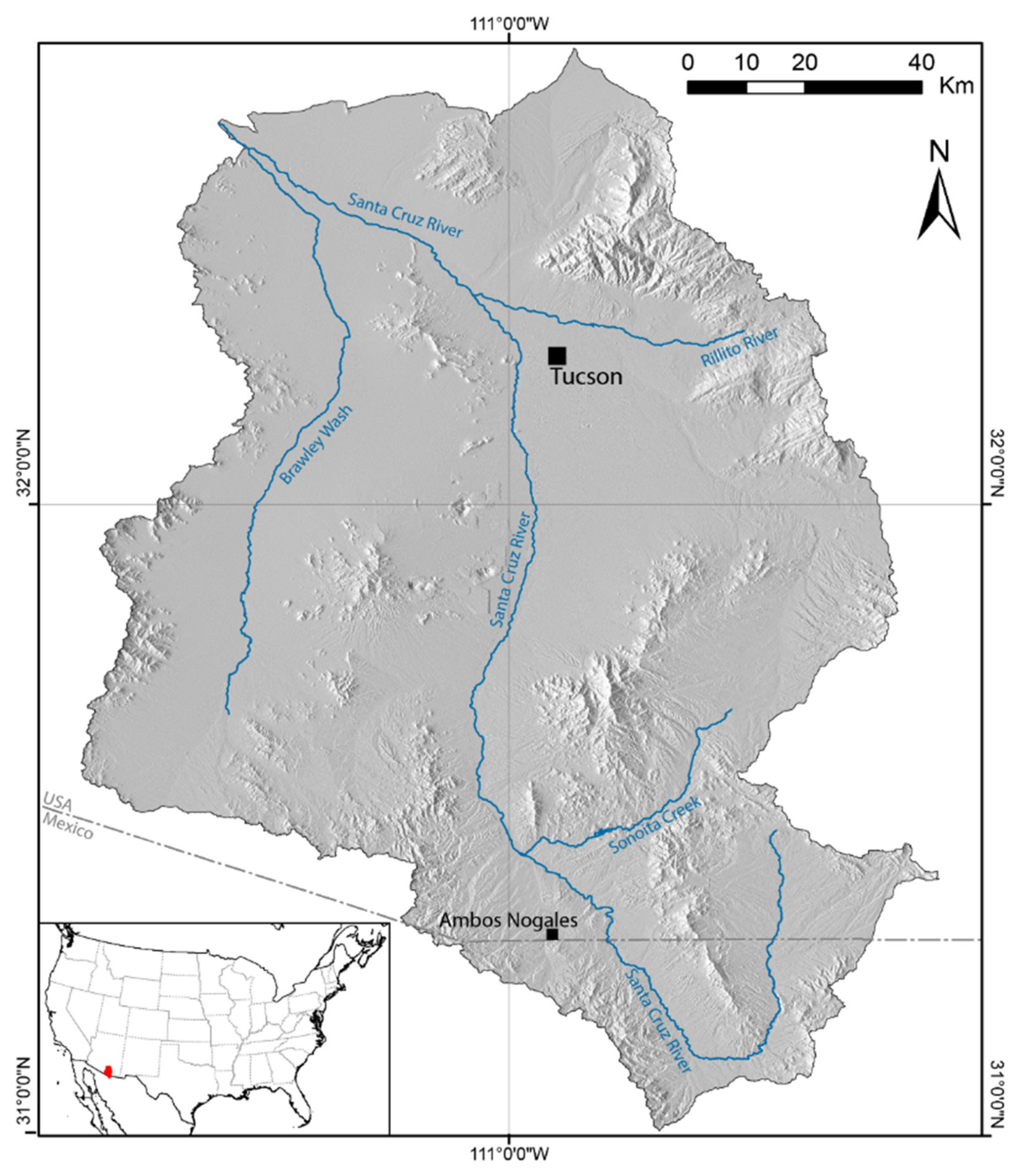
Figure 1. Study Area, Upper Santa Cruz Watershed. Hill shade base map derived from [43], streams and watershed boundaries from [44] and administrative division from [45].
Remotesensing 14 02127 g001
Figure 2. Google Earth Engine workflow scheme for yearly LULC classification (Pre-processed yearly biseasonal Landsat scenes were exported between each step not to overflow the server’s computing capacities [42]).
Remotesensing 14 02127 g002
Figure 3. Average variable importance over the 35 yearly Random Forest classification models. Top 40 variables are the ones with the highest mean contribution over our 35 yearly classifications.
Remotesensing 14 02127 g003
Figure 4. LULC change dynamics showing (a) land cover in 1986, (b) land cover in 2020, (c) major changes between 1986 and 2020 and (d) the intensity of change during the 1986–2020 period, which refers to the number of times the pixel changed major classes.
Remotesensing 14 02127 g004
Figure 5. Natural land cover changes (1986–2020); note that the gap in the figure corresponds to the year 2012 which was not mapped. Wildfire extent is represented here [83], may be of various burn severity.
Remotesensing 14 02127 g005
Figure 6. Human-driven land cover changes (1986–2020); note that the gap in the figure corresponds to the year 2012 which was not mapped.
Remotesensing 14 02127 g006
Figure 7. Monitoring sudden and gradual land cover changes following the Florida wildfire (2005) south of Tucson. Burn boundaries extracted from [83], hillshade basemap derived from [43].
Remotesensing 14 02127 g007
Figure 8. Urban extension in the upper Santa Cruz watershed from 1986 to 2020. Hillshade derived from [43], census designated places from [84] and United States–Mexico border from [45].
Remotesensing 14 02127 g008
Table 1. Names, formulas and references for indices, Landsat data transformations and ancillary data used as predictor variables in land cover classifications.
VariableFormulaRefs.
Normalized Difference Vegetation Index (NDVI) NIR     Red NIR   +   Red [56]
Normalized Difference Water Index (NDWI) NIR     SWIR NIR   +   SWIR [57]
Normalized Difference Built-up Index (NDBI) SWIR     NIR SWIR   +   NIR [58]
Built-up Area Extraction Index (BAEI) Red   +   0.3 Green   +   SWIR [58]
Normalized Difference Bareness Index (NDBai) SWIR     TIR SWIR   +   TIR [58]
Dry Built-up Index (DBI) Blue     TIR Blue   +   TIR     NDVI [59]
Dry Bare-Soil Index (DBSI) SWIR     Green SWIR   +   Green     NDVI [59]
Topographic Position Index (TPI)Elevation—Mean
(Elevation in 15 pixel radius)
[43,60,61,62]
Gray-Level Co-Occurrence Matrix (GLCM) Textural Correlation i , j p i , j i µ i j µ j σ i 2 σ j 2 [63]
Gray-Level Co-Occurrence Matrix (GLCM) Textural Contrast i , j |   i j   | 2   p i , j [63]
Multitemporal Kauth-Thomas (MKT)See references[64,65,66]
Table 2. Land use and land cover classes description.
ClassDescription (Percentages Are Indicative)
11. WaterArea dominated by open water (>50%).
21. Developed, RoadsMixture of constructed material (<20%) and vegetation.
22. Urban, Low DensityMixture of constructed material (20 to 50%) and vegetation.
23. Urban, Medium DensityMixture of constructed material (50 to 80%) and vegetation.
24. Urban, High DensityMostly constructed material (80 to 100%).
31. Barren, WashesBarren lands (vegetation < 15%) in intermittent streams washes (Arroyos).
32. Barren, MinesBarren lands (vegetation < 15%) in mines (pits, tailings, etc.).
41. Deciduous ForestArea dominated by mesquite (>20%) greater than 2 m tall and shedding their foliage. Mostly along floodplains and arroyos.
42. Evergreen ForestArea dominated by trees (>20%) greater than 5 m tall with permanent foliage. Mostly oaks, junipers and pine.
43. Rocky Outcrops1Occasional outcrops of bedrock in evergreen-dominated areas.
52. ShrubsArea dominated by shrubs and cacti (>20%) less than 5 m tall.
53. Shrubs, Dark1Shrubs on dark, volcanic ground influencing spectral signature.
54. Shrubs, Bright1Shrubs on bright, sandy ground influencing spectral signature.
71. GrasslandAreas dominated by graminoid or herbaceous vegetation (>80%). Natural vegetation which can be used for grazing.
81. Pasture and ParksPerennial areas of grasses (>20%) planted for livestock grazing or for recreational areas (parks, golfs, etc.).
82. Cultivated CropsAreas used for the production of annual crops (>20%).
83. Nut-Tree Plantations1Areas used for the production of nuts trees (>20%), mostly pecan.
91. Riparian ForestAreas dominated by woody vegetation (>20%) greater than or equal to 5 m in height. Mostly cottonwoods in arroyos.
1 Subclasses to catch local variations of their parent class for the classification but merged after.
Table 3. 1986–2020 cumulative yearly identified changes matrix (initial land cover in lines, final land cover in columns, values are percentages of all detected changes totaling 27,318,648 pixel counts).
Classes1121222324313241425271818291Total
11. Water 0.00%0.00%0.00%0.00%0.00%0.02%0.01%0.01%0.00%0.00%0.00%0.00%0.00%0.06%
21. Developed. Roads 0.11%0.01%0.05% 0.17%
22. Urban. Low Density 0.16% 1.38%0.35% 1.89%
23. Urban. Med. Density 0.02%1.43% 0.43% 1.88%
24. Urban. High Density 0.05%0.26%0.50% 0.81%
31. Barren. Washes0.00%0.02%0.10%0.02%0.03% 0.13%1.00%0.06%1.93%0.10%0.04%0.04%0.07%3.55%
32. Barren. Mines0.03%0.01%0.20%0.26%0.17%0.10% 0.03%0.03%1.13%0.00%0.01%0.01%0.00%1.98%
41. Deciduous Forest0.01%0.09%0.14%0.00%0.01%0.73%0.04% 5.16%14.43%7.49%0.08%0.19%0.37%28.75%
42. Evergreen Forest0.01%0.01%0.04%0.01%0.00%0.06%0.02%4.47% 2.41%0.02%0.00%0.01%0.07%7.13%
52. Shrubs0.01%0.19%1.14%0.22%0.14%1.71%1.37%14.63%2.18% 9.91%0.13%0.49%0.00%32.13%
71. Grassland0.00%0.00%0.01%0.00%0.00%0.09%0.01%7.74%0.02%11.33% 0.01%0.03%0.00%19.23%
81. Pasture and Parks0.00%0.00%0.05%0.01%0.01%0.03%0.01%0.09%0.00%0.04%0.00% 0.17%0.01%0.42%
82. Cultivated Crops0.00%0.00%0.02%0.00%0.00%0.04%0.01%0.26%0.01%0.57%0.04%0.18% 0.04%1.17%
91. Riparian Forest0.00%0.00%0.01%0.00%0.00%0.10%0.00%0.53%0.12%0.02%0.00%0.01%0.04% 0.84%
Total0.06%0.55%3.51%2.42%1.20%2.87%1.61%28.75%7.60%31.86%17.57%0.46%0.98%0.57%
Publisher’s Note: MDPI stays neutral with regard to jurisdictional claims in published maps and institutional affiliations.