Adaptive Max-Margin One-Class Classifier for SAR Target Discrimination in Complex Scenes

Abstract

Synthetic aperture radar (SAR) target discrimination is an important stage that distinguishes targets from clutters in the radar automatic target recognition field. However, in complex SAR scenes, the performance of some traditional discriminators will degrade. As an effective tool for one-class classification (OCC), the max-margin one-class classifier has attracted much attention for SAR target discrimination, as it can effectively reduce the impact of multiple clutters. However, the performance of the max-margin one-class classifier is very sensitive to the values of kernel parameters. To solve the problem, this paper proposes an adaptive max-margin one-class classifier for SAR target discrimination in complex scenes. In a max-margin one-class classifier with a suitable kernel parameter, the distance between a sample and classification boundary satisfies a certain geometric relationship, i.e., edge samples in input space are transformed to the region in the kernel space close to boundary, while interior samples in input space are transformed to the region in the kernel space far away from boundary. Therefore, we define the information entropy of samples in the kernel space to measure the distance between samples and classification boundary. To automatically obtain the optimal kernel parameter of the max-margin one-class classifier, the edge and interior samples in the input space are first selected, and then the parameter optimization is performed by minimizing information entropy of interior samples and simultaneously maximizing the information entropy of edge samples. Experimental results of the synthetic datasets and measured synthetic aperture radar (SAR) datasets validate the effectiveness of our method.

1. Introduction

The development of synthetic aperture radar (SAR) imaging technology has resulted in great attention to the field of SAR automatic target recognition (ATR) [1,2]. The SAR ATR system usually contains three basic stages [3,4]: detection [5,6,7], discrimination [8,9,10], and recognition [11,12]. The target detection stage aims to locate the targets of interest and obtain the candidate target results, which contain the true targets and some clutters. The main task of target discrimination is to remove the false alarm clutters from the candidate target results and reduce the burden of the recognition stage that identifies the target type. As the second stage of SAR ATR, target discrimination performs an important role in SAR ATR systems and receives lots of attention in the remote sensing images processing field.

Many target discrimination methods have been developed, and many traditional target discrimination methods mainly focus on discriminative feature extraction. In [8], Wang et al. propose a superpixel-level target discrimination method that uses the multilevel and multidomain feature descriptor to obtain the discriminative features. Wang et al. [9] extract the local SAR-SIFT features that are then encoded to improve the category-specific performance. Moreover, Li et al. [10] develop a discrimination method by extracting the scattering center features of SAR images, which can effectively identify the targets from clutters. Although these methods [8,9,10] perform well on SAR target discrimination, they ignore the design of discriminators, which may restrict their discrimination performance in complex scenes.

Several classifiers have been proposed to solve one-class classifier (OCC) problems and have been applied for discrimination. They can be categorized into three groups: statistical methods, reconstruction-based methods, and boundary-based methods. In statistical methods, the probability density function (PDF) [13] of the target samples is estimated firstly, and then a threshold is predefined to determine whether test samples are generated from this distribution. Reconstruction-based methods, such as Auto-encoder (AE) and variational AE [14], learn a representation model by minimizing the reconstruction errors of the training samples from the target class; the reconstruction errors of test samples are then used to judge whether they belong to the target class. In boundary-based methods [15,16], a boundary is constructed with the training samples only from target class to determine the region where the target samples are located. The most well-known boundary-based method are max-margin one-class classifiers, i.e., one-class support vector machine (OCSVM). As discussed above, statistical methods are simple and carried out by estimating the probability density of the target sample distribution, but they rely on a large number of training samples to estimate a precise probability density, especially when the dimension of training data are high. In addition, reconstruction-based methods are effective and explore the representative features for one-class classification, but they also need sufficient training samples in order to learn a suitable model for the target samples. In OCSVM, the kernel transformation makes them handle nonlinear data easily, the relaxation items make them generalize well, and the sparse support vectors help them save a lot of storage space, thus they have gained significant attention for solving OCC problem. However, the performance of the OCSVM is very sensitive to the values of the kernel parameters.

Recently, several methods [17,18,19] have been developed to select the suitable kernel parameters for OCSVM. First, a kernel parameter candidate set is predefined and the value of objective function for each element in the candidate set is computed. Next, the optimal kernel parameter is selected based on the minimum/maximum objective function values. In [17], Deng et al. propose a method referred to as SKEW for OCSVM based on the false alarm rate (FAR) and missing alarm rate (MAR). Wang et al. [18] introduce a MinSV+MaxL method for SVDD, which computes the objective function value $V_L$ and the proportion $V_s$ between the support vectors and training samples for each element in the parameter candidate set, and the optimal parameter is determined by the maximum difference between adjacent times of $V_L$ and $V_s$. Xiao et al. [19] put forward a MIES method for OCSVM via the distance between the sample and classification boundary. Although the methods [17,18,19] can select a suitable Gaussian kernel parameter, they suffer from two main challenges: (1) it is difficult to predefine the kernel parameter candidate set in the range of $(0,+\infty )$; (2) the computing burden of these methods is large, since the value of objective function is computed for each parameter in the candidate set, especially when there are many elements in the candidate set. Consequently, these kernel parameter selection methods still restrict the performance of the one-class classifier.

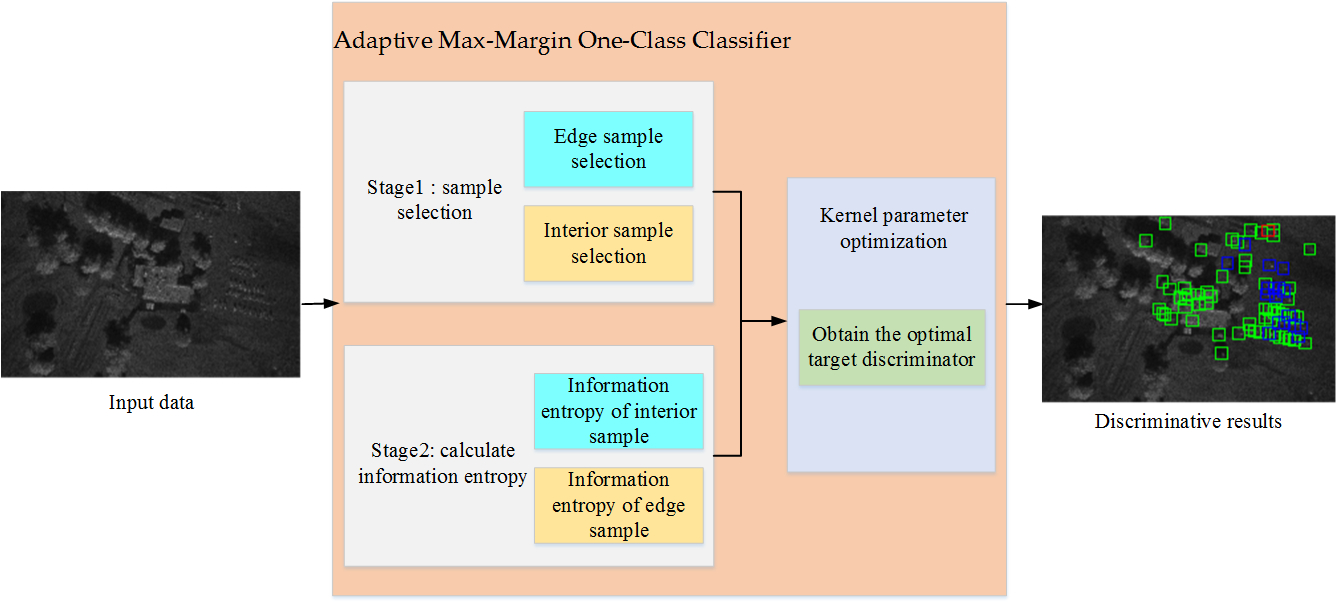
To access the above issues, this paper aims to develop an adaptive max-margin one-class classifier by automatically obtaining the optimal kernel parameter, which is adaptive to the complex scenes of SAR images. The motivations of our method are as follows:

(1)

An adaptive max-margin one-class classifier is developed for SAR target discrimination in complex scenes, in which a suitable kernel parameter of the max-margin one-class classifier is learned based on the geometric relationship between the sample and classification boundary without a parameter candidate set. In this way, the proposed method can not only achieve the promising discrimination performance, but also avoid the difficulty of determining the parameter candidate set and reduce the computational cost in the training stage. In detail, for the max-margin one-class classifier, the training samples in the input space are mapped to the kernel space via the kernel transformation. Then, the classification boundary is constructed in the kernel space via the samples that are closest to the classification boundary, i.e., support vectors (SVs). 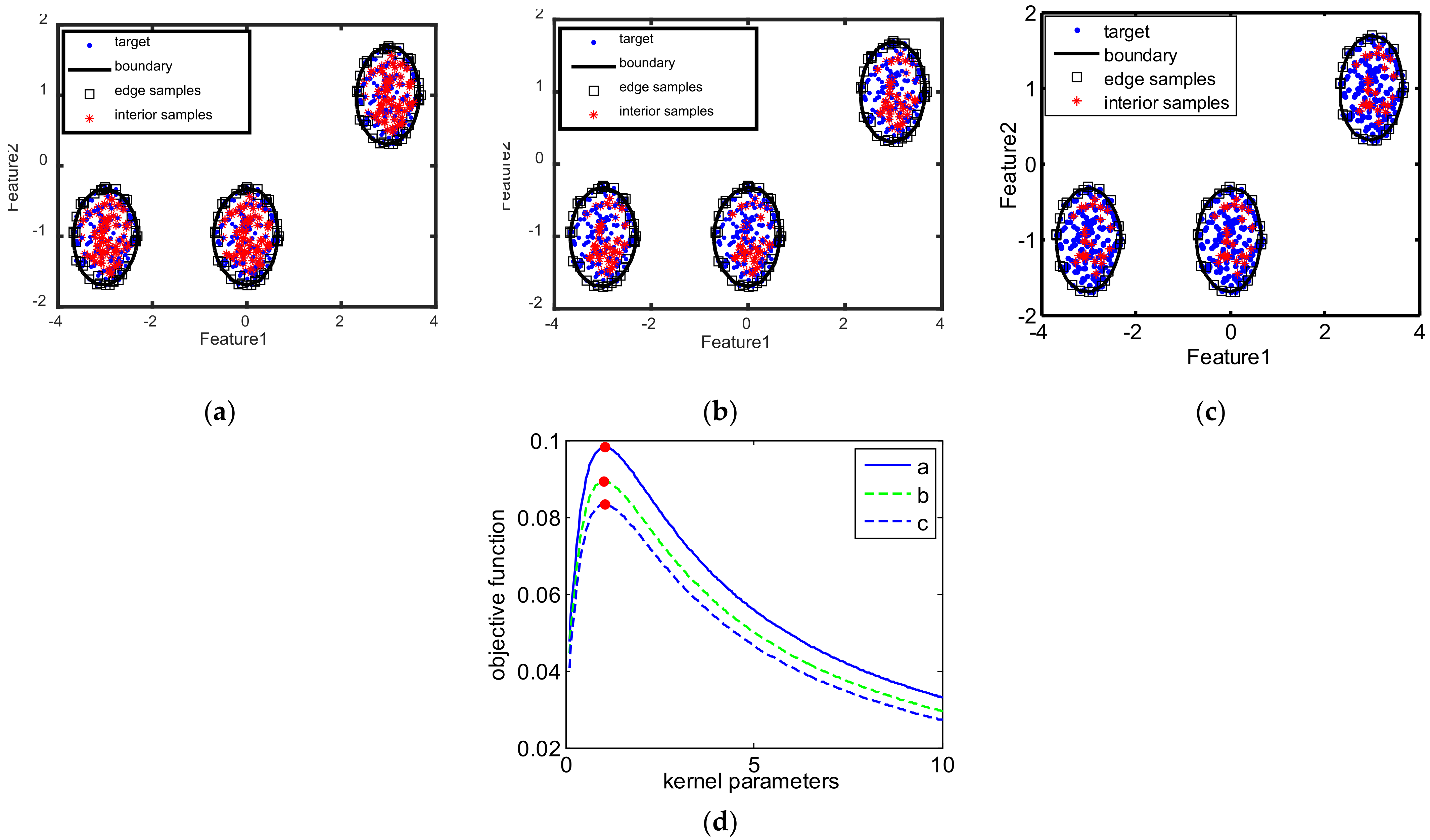As discussed in [20], with a suitable kernel parameter, the max-margin one-class classifier can ensure that the edge samples in the input space are transformed to the region in the kernel space close to the classification boundary and more likely to become SVs, and the interior samples in the input space are transformed to the region in the kernel space far away from the boundary and unlikely to become the SVs. Thus, an optimal kernel parameter for the max-margin one-class classifier can be adaptively obtained based on the above geometric relationship.

(2)

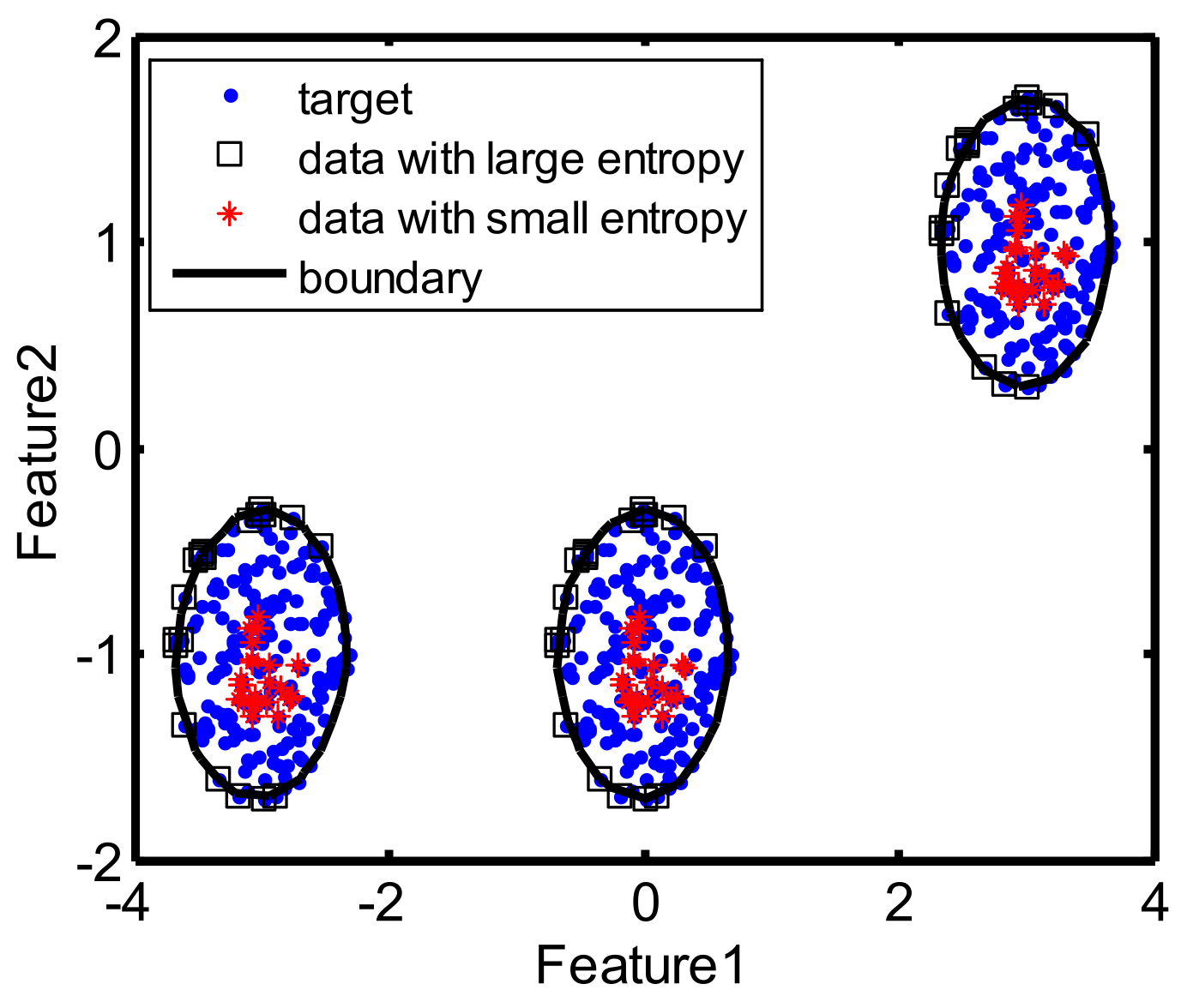
We define the information entropy of samples as the objective function of our method, which measures the distance between a sample and the classification boundary in the kernel space that can be automatically optimized by the gradient descent algorithm. Specifically, the larger entropy value a sample has, the closer the sample is to the classification boundary. The optimal kernel parameter can be learned by maximizing the information entropy of edge samples and simultaneously minimizing the information entropy of interior samples. In this way, the optimal kernel parameter can ensure that the edge samples in the input space are projected to the area in the kernel space close to the classification boundary, while the interior samples in the input space are projected to the area in the kernel space far away from the classification boundary. Based on the above criterion, our method can obtain the optimal kernel parameter that further devotes to the promising discrimination performance.

This paper focuses on the exploration of an adaptive max-margin one-class classifier for SAR target discrimination in complex scenes, and the main contributions of this paper are summarized as: (1) the geometric relationship between the sample and classification boundary is utilized to learn a suitable kernel parameter for OCSVM without a parameter candidate set, which can effectively reduce the computational cost in the training stage and ensure a favourable performance for SAR target discrimination; (2) the information entropy is defined for each sample to measure the distance between a sample and the classification boundary in the kernel space, which is adopted as the objective function of our method that can be automatically optimized by the gradient descent algorithm.

The remainder of this paper is organized as follows: a review about max-margin one-class classifiers is given in Section 2, and the proposed method is presented in Section 3. In Section 4, some experimental results on synthetic datasets and measured synthetic aperture radar (SAR) datasets are presented. Finally, Section 5 and Section 6 describe the discussion and conclusions, respectively.

2. Max-Margin One-Class Classifier

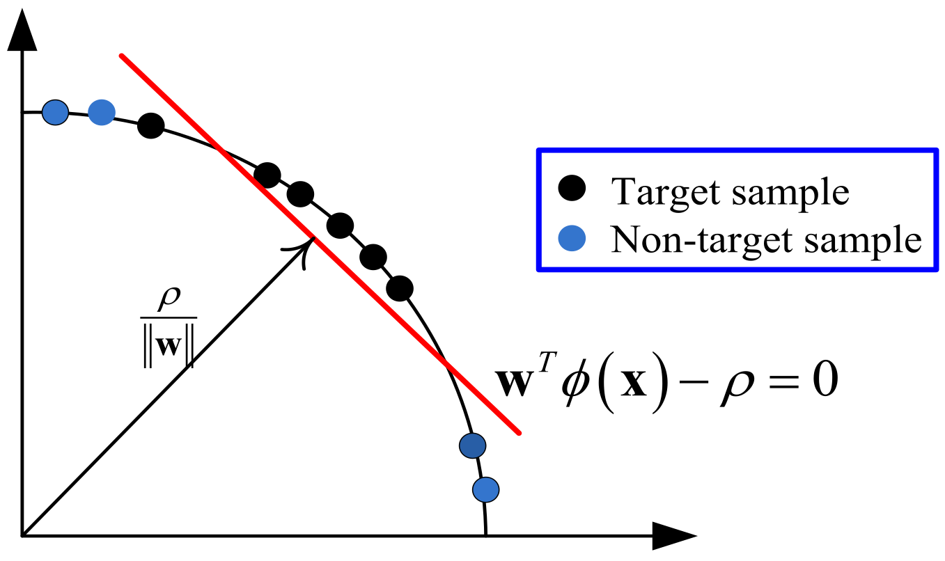
One-class SVM is a domain-based classification method that looks for the classification hyperplane to set the boundary of the target class sample; most of the training samples are located above the hyperplane, and the distance from the origin to the hyperplane is the largest. The maximum distance from the origin to the hyperplane is called the “maximum-margin”, so the OCSVM is also called the max-margin one-class classifier. The 2D illustrations of OCSVM are shown in Figure 1.

The objective function of OCSVM is shown in Equation (1):

$$\begin{array}{l}\underset{w,{\xi }_i,\rho }{\min }\frac{1}{2}{‖w‖}^2+\frac{1}{\eta N}{\displaystyle \sum _i{\xi }_i}-\rho \\ \mathrm{s}.\mathrm{t}.\left(w^T{\tilde{x}}_i\right)\ge \rho -{\xi }_i;{\xi }_i\ge 0,\forall i\end{array}$$

(1)

with $w$ being the slope of the classification hyperplane, $\eta$ being a tradeoff parameter, and ${\xi }_i$ the slack term. Moreover, ${\tilde{x}}_i$ is represented as follow:

$${\tilde{x}}_i=\left[\kappa \left(x_i,r_1\right),\kappa \left(x_i,r_2\right),\cdots ,\kappa \left(x_i,r_M\right)\right]$$

(2)

where $\kappa \left(\cdot ,\cdot \right)$ denotes the kernel function. As a most widely used feature transformation, Gaussian kernel transformation possesses the special characteristics of similarity preserving and its value is $0<\kappa \left(\cdot ,\cdot \right)\le 1$. The Gaussian kernel transformation transforms the data in input space into the unit hypersquare of the first quadrant in the kernel sparse. The target samples are transformed to the region far away from the origin, while the clutter samples are projected into the region near the origin.

For dataset ${\left\{x_i\right\}}_{i=1}^N$, Gaussian kernel function defines the inner product of two samples in the kernel space, and thus, $\kappa \left(\cdot ,\cdot \right)$ can be further formulated as:

$$\kappa \left(x_i,x_j\right)=〈\varphi \left(x_i\right),\varphi \left(x_j\right)〉=\exp \left(-\frac{{‖x_i-x_j‖}_2^2}{2{\sigma }^2}\right)$$

(3)

where $\varphi \left(\cdot \right)$ is the Gaussian kernel transformation without explicated expression, and $\sigma$ is the Gaussian kernel parameter. It is obvious that $〈\varphi \left(x_i\right),\varphi \left(x_i\right)〉=\exp \left(0\right)=1$, thus $‖\varphi \left(x_i\right)‖=1$ for every samples. In other words, samples are mapped to the unit hypersphere in the kernel space with Gaussian kernel transformation. Moreover, the cosine of the central angle between two samples in the kernel space, i.e., $\cos \theta =\frac{〈\varphi \left(x_i\right),\varphi \left(x_j\right)〉}{‖\varphi \left(x_i\right)‖‖\varphi \left(x_j\right)‖}=〈\varphi \left(x_i\right),\varphi \left(x_j\right)〉=\kappa \left(x_i,x_j\right)$. Therefore, the value of $\kappa \left(x_i,x_j\right)$ measures the similarity of two samples in the kernel space.

Different values of Gaussian kernel parameters correspond to different distributions of samples in the kernel space. On the consideration of two extreme cases–$\sigma \to +\infty$ and $\sigma \to 0$–we can see that $\kappa \left(x_i,x_j\right)$ is very close to 1 for any paired-samples when $\sigma \to +\infty$, thus the cosine of the angle between two samples in the kernel space is close to 1. In other words, all samples are mapped to the same location in the kernel space if $\sigma \to +\infty$. On the contrary, $\kappa \left(x_i,x_j\right)$ is close to 0 for any paired samples when $\sigma \to 0$, thus the cosine of the angle between two samples in the kernel space is close to 0. Therefore, all samples are mapped to the edge of each quadrant in the kernel space if $\sigma \to 0$. Since different values of Gaussian kernel parameters correspond to the different distributions of samples in the kernel space, the decision boundaries of OCSVM are different when the selection of Gaussian kernel parameters are different.

In addition, Equation (1) can be transformed as Equation (4) via Lagrange multiplier theory:

$$\begin{array}{l}\underset{\alpha }{\min }{\displaystyle \sum _{i,j}^N\frac{1}{2}{\alpha }_i{\alpha }_j\kappa \left(x_i,x_j\right)}\\ \mathrm{s}.\mathrm{t}.0\le {\alpha }_i\le \frac{1}{\eta N},\forall i{\displaystyle \sum _{i=1}^N{\alpha }_i}=1\end{array}$$

(4)

The problem of Equation (4) can be solved with a sequential minimal optimization (SMO) algorithm [21]. Once the optimal solution $\alpha$ is obtained, the decision function of OCSVM is given in Equation (5):

$$f(x^{\ast })=sign\left({\displaystyle \sum _{i=1}^N{\alpha }_i\kappa \left(x_i,x^{\ast }\right)}-\rho \right)$$

(5)

The test samples $x^{\ast }$ belongs to the target class in the case of $f(x^{\ast })\ge 0$. Otherwise, $x^{\ast }$ belongs to the non-target class. It is can be seen from Equation (5) that the parameters of classification boundary in OCSVM are determined by the samples with coefficient $\alpha$ larger than 0, i.e., SVs. In other words, the classification boundary of OCSVM is decided via SVs, which is aligned with the analysis in the Introduction. According to the above analysis, this paper chooses the Gaussian kernel function for the max-margin one-class classifier.

3. The Proposed Method

In this section, a detailed introduction to our method will be shown. In Section 3.1, the algorithm of interior and edge samples selection is first presented. Then, the definition of information entropy for each sample in the kernel space is shown in Section 3.2. Finally, the objective function for automatically learning the optimal kernel parameter is given in Section 3.3.

3.1. Sample Selection

First of all, our method chooses the edge and interior samples in the input space. For 2D data, we can manually select samples via visual results of data distribution, but it is beyond our reach to manually select samples in high-dimensional space. Therefore, an algorithm that can automatically select edge and interior samples is a key step in our method.

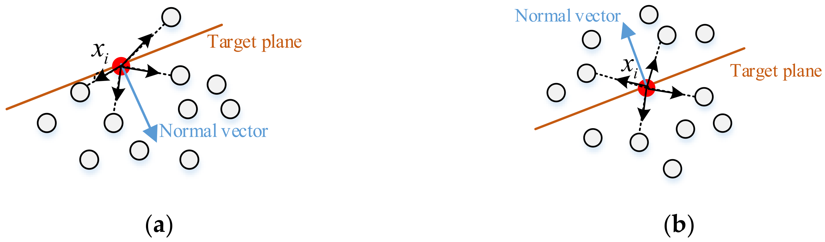
In general, for an interior sample $x_i$, its nearest neighbors are evenly sitting on two sides of the tangent plane passing through $x_i$. On the contrary, most of the nearest neighbors of an edge sample $x_i$ only sit on one side of the tangent plane passing through $x_i$. Such local geometric information between the samples and their nearest neighbors can be used for the selection of interior and edge samples. 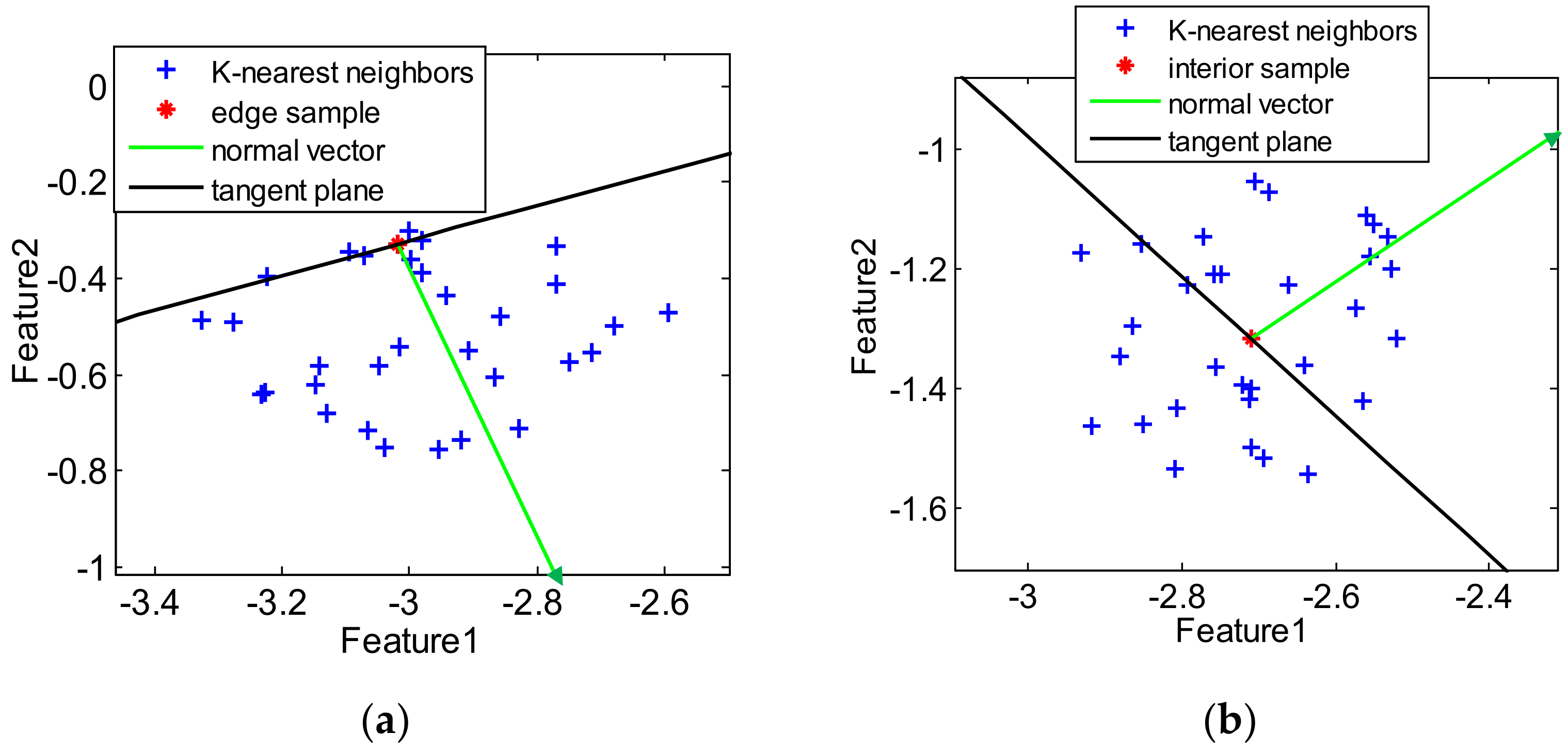We should point out that the edge sample selection idea is from article [22], while the idea of interior sample selection is further induced in this paper. To give an illustration to the geometric relation, Figure 2 presents the schematic of an edge sample and an interior sample, including their k-nearest neighbors, normal vectors, and target tangent planes.

In detail, based on the $k$-nearest neighbors of the sample $x_i$, the normal vector $V_i$ of the tangent plane passing through sample $x_i$ can be approximated as follows:

$$V_i={\displaystyle \sum _{j=1}^K\frac{x_{ij}-x_i}{‖x_{ij}-x_i‖}}$$

(6)

where $x_{ij}$ is the $j$th neighbor of $x_i$. Then, the dot products between the normal vector and the vectors from $x_i$ to its k-nearest neighbors can be computed:

$${\theta }_{ij}={\left(x_{ij}-x_i\right)}^T{V}_i$$

(7)

Thus, the fraction of nonnegative dot products is calculated based on ${\theta }_{ij}$:

$$l_i=\frac{1}{K}{\displaystyle \sum _{j=1}^{K}I\left({\theta }_{ij}>0\right)}$$

(8)

In Figure 2b, the nearest neighbors sit evenly on two sides of the tangent plane for the interior sample. Consequently, the value of $l_i$ is close to 0.5. On the contrary, as shown in Figure 2a, most of the nearest neighbors of the edge sample sit only on one side of the tangent plane. Therefore, the value of $l_i$ is close to 1. In other words, the criterion of selecting the edge and interiors samples is expressed as:

$$\left\{\begin{array}{l}{x}_i\mathrm{is}\mathrm{an}\mathrm{edge}\mathrm{sample}\mathrm{if}{l}_i>1-\gamma \\ x_i\mathrm{is}\mathrm{an}\mathrm{interior}\mathrm{sample}\mathrm{if}0.5-\eta <l_i<0.5+\eta \end{array}\right.$$

(9)

where $\gamma$ and $\eta$ are predefined parameters with small values.

For the sample selection algorithm, there are three predefined parameters: $K,\gamma ,\eta$. When the value of $\eta$ is 0, all of the nearest neighbors of a sample sit evenly on two sides of its tangent plane. Similarly, when the value of $\gamma$ is 0, all of the nearest neighbors of a sample are only located on one side of the tangent plane. Such requirements for sample selection are too strict. Therefore, the requirements for selecting samples are loose by setting small values for parameters $\gamma$ and $\eta$. Empirically, as discussed in reference [22], we set the range of the parameters $\gamma$ and $\eta$ as $[0,0.1]$. For the parameter $K$, the values of parameter $K$ affects the estimation accuracy of the normal vector, and a recommended value is $K=5\ln N$ [14], with $N$ being the number of training data.

3.2. Information Entropy of Samples

In the max-margin one-class classifier, the SVs are sparsely located on the decision boundary in the kernel space, while the interior samples are densely distributed inside the decision boundary. Therefore, if samples are close to the decision boundary, they are located in the low-density region and far away from most of other samples, and more likely to be CVs [13]. On the contrary, if samples are far away from the decision boundary, they are located in the high-density region and close to most of other samples [14].

For the samples, we can calculate the Euclidean distance between two samples in the kernel space as:

$$di{s}_{ij}={‖\varphi \left(x_i\right)-\varphi \left(x_j\right)‖}^2=\kappa \left(x_i,x_i\right)+\kappa \left(x_j,x_j\right)-2\kappa \left(x_i,x_j\right)$$

(10)

with $x_i$ and $x_j$ denoting two samples in the training set and $\kappa \left(x_i,x_j\right)$ the kernel function. As discussed in Section 2, we choose the Gaussian kernel function for $\kappa \left(x_i,x_j\right)$, and then, Equation (10) can be approximated as:

$$di{s}_{ij}=2\left(1-\kappa \left(x_i,x_j\right)\right)$$

(11)

which represents the Euclidean distance between the samples $x_i$ and $x_j$.

Then, the probability of dissimilarity between $x_i$ and $x_j$ is defined via $di{s}_{ij}$:

$$p_{ij}=\frac{di{s}_{ij}}{{\displaystyle \sum _{n=1}^{N}di{s}_{in}}}$$

(12)

with $N$ denoting the number of samples in the training set. For a sample $x_i$, if it is located close to the decision boundary and far from most other samples $x_j$, most of the values ${\left\{di{s}_{ij}\right\}}_{j=1}^N$ are very big, and thus the probability of dissimilarity $p_{ij}$ is approximate to $1/N$; if $x_i$ is far from the decision boundary and close to most of the other samples $x_j$, most of the values ${\left\{di{s}_{ij}\right\}}_{j=1}^N$ are very small, and thus the probability of dissimilarity $p_{ij}$ is approximately to 0 or 1.

Finally, the information entropy function related to the samples’ Euclidean distance is defined for $i\mathrm{th}$ sample based on the probability of dissimilarity $p_{ij}$:

$$H_i=-{\displaystyle \sum _{j=1}^N{p}_{ij}{\log }_2{p}_{ij}}$$

(13)

To solve the problem of $\log 0$ in Equation (13), we set $p_{ii}=1$ instead of 0, and then the terms $p_{ii}{\log }_2{p}_{ii}=0$ do not impact the calculation of other terms $p_{ij}{\log }_2{p}_{ij}=0(j\ne i)$ for $H_i$. According to the property of information entropy, Equation (13) shows that, for sample $x_i$ close to the decision boundary with its probability of the dissimilarity $p_{ij}$ approximate to $1/N$, the entropy value $H_i$ is very large; for sample $x_i$ far from the decision boundary with its probability of the dissimilarity $p_{ij}$ approximate to 0 or 1, the entropy value $H_i$ is very small. With the above analysis, the larger entropy value a sample has, the closer the sample is to the decision boundary. Thus, the information entropy of samples in Equation (13) can be utilized to measure the distance between the samples with the decision boundary in the kernel space.

3.3. Objective Function of the Proposed Method

As analyzed in [19,20], for an appropriate kernel parameter, the distance between samples and classification boundary satisfies a certain geometric relationship for the max-margin one-class classifier, i.e., the edge samples in the input space are transformed to the region in the kernel space close to boundary and more likely to become SVs, while the interior samples in the input space are transformed to the region in the kernel space far away from boundary and unlikely to become SVs. In Section 3.2, we can see that the samples with large entropy values are close to boundary and more likely become SVs, while samples with small entropy values are far away from decision boundary and unlikely to become SVs. Therefore, for an appropriate kernel parameter, the entropy values of edge samples are high, while the entropy values of interior samples are low. Based on the above analysis, the optimal kernel is obtained via maximizing the subtraction of information entropy between the edge and interior samples. The objective function of our method is shown as:

$${\sigma }_{opt}=\underset{\sigma }{\arg \max }\left\{\frac{1}{N_1}{\displaystyle \sum _{i\in C_1}H\left(x_i;\sigma \right)}-\frac{1}{N_2}{\displaystyle \sum _{j\in C_2}H\left(x_j;\sigma \right)}\right\}$$

(14)

where $H\left(x_i;\sigma \right)$ represents the entropy value of $x_i$ with kernel parameter $\sigma$, and $C_1$ and $C_2$ representing the set of edge samples and interior samples, respectively; $N_1$ and $N_2$ represent the number of edge samples and interior samples, respectively. By maximizing the information entropy of edge samples and minimizing the information entropy of interior samples, we ultimately obtain the optimal kernel parameter. The optimization of Equation (13) can be solved via the gradient descent algorithm. The gradient of Equation (14) with respect to parameter $\sigma$ is given in Equation (15):

$$\begin{array}{l}\frac{\partial J}{\partial \sigma }=\frac{1}{N_1}{\displaystyle \sum _{i\in C_1}\frac{\partial H\left(x_i;\sigma \right)}{\partial \sigma }}-\frac{1}{N_2}{\displaystyle \sum _{j\in C_2}\frac{\partial H\left(x_j;\sigma \right)}{\partial \sigma }}\\ \frac{\partial H\left(x_i;\sigma \right)}{\partial \sigma }=-{\displaystyle \sum _{n=1}^N\left\{\left(1+{\log }_2{p}_{in}\right)\frac{{\upsilon }_{in}{\displaystyle \sum _{k=1}^{N}di{s}_{ik}}-di{s}_{in}{\displaystyle \sum _{k=1}^N{\upsilon }_{ik}}}{{\left({\displaystyle \sum _{k=1}^{N}di{s}_{ik}}\right)}^2}\right\}}\\ {\upsilon }_{ik}=\frac{1}{2}{‖x_i-x_k‖}^2\exp \left(-\frac{{‖x_i-x_k‖}^2}{2{\sigma }^2}\right)\end{array}$$

(15)

where $di{s}_{ik}$ is the square of Euclidean distance of two samples $x_i$ and $x_k$ in the kernel space, and $p_{in}$ is the similarity between $x_i$ and $x_n$. The formulations of $di{s}_{ik}$ and $p_{in}$ are predefined in Section 3.2. We summarize the whole procedure of our method in Algorithm 1.

Algorithm 1. The procedure of the proposed method

1: Input: Training set ${\left\{x_i\right\}}_{i=1}^N$, $K$, $\gamma$, $\eta$, $\delta$, initial value $\sigma ={\sigma }_0$, threshold $\epsilon$. 2: Output: the optimal kernel parameter ${\sigma }_{opt}$. 3: for $n=1:N$ 4:  Select the k-nearest neighbors of sample $x_i$: ${\left\{x_{ij}\right\}}_{j=1}^K$; 5:  Compute the normal vector $V_i$ of the tangent plane passing through $x_i$ based on Equation (6); 6:  Compute the fraction of nonnegative dot products $l_i$ based on Equation (8); 7: end for 8: Construct the set of edge samples $C_1$ and the set of interior samples $C_2$ based on Equation (9); 9: While $Diff>\epsilon$ 10:  Calculate the gradient functions $\partial J/\partial \sigma$ based on Equation (14); 11:  ${\sigma }^{new}={\sigma }^{old}+\delta \frac{\partial J}{\partial \sigma }$; 12:  Calculate the value of objective function $O{F}^{new}$ based on Equation (13); 13:  $Diff=\frac{\left|O{F}^{new}-O{F}^{old}\right|}{O{F}^{old}}$ 14:  ${\sigma }^{old}$=${\sigma }^{new}$, $O{F}^{old}=O{F}^{new}$; 15: End 16: Output: the optimal kernel parameter ${\sigma }_{opt}$.

4. Results

To validate the target discrimination performance of our method, the synthetic datasets, UCI datasets, and measured synthetic aperture radar (SAR) dataset are used in this section. Three kernel parameter selection methods including MIES [19], MinSV+MaxL [18], and SKEW [17]–a parameter learning method referred to as MD [23]–are used to compare with our method. For parameter selection methods, the parameter candidate set for selection is set as $[0.1,10]$ with the interval of 0.1. For our method, the initial kernel parameter is set as 1. Moreover, some other discriminators, including k-means clustering [24], principle component analysis (PCA) [25], minimum spanning tree (MST) [26], Self-Organizing Map (SOM) [27], Auto-encoder (AE) [14], the minimax probability machine (MPM) [28], and two-class SVM [29], are also taken as comparisons from which to illustrate the promising performance of our method.

In the OCC problem, the confusion matrix reflects the primary source of the results, which is presented in

Table 1. The confusion matrix for the OCC problem.

		Predicted Class
		1	0
True class	1	True Positive (TP)	False Negative (FN)
	0	False Positive (FP)	True Negative (TN)

.

The measurement standards of classification precision, recall, F1score, and accuracy are defined as:

$$\begin{array}{l}\mathrm{precision}=\frac{\mathrm{TP}}{\mathrm{TP}+\mathrm{FP}}\\ \mathrm{recall}=\frac{\mathrm{TP}}{\mathrm{TP}+\mathrm{FN}}\\ \mathrm{F}1\mathrm{score}=\frac{2\times \mathrm{percision}\times \mathrm{recall}}{\mathrm{percision}+\mathrm{recall}}\\ \mathrm{accuracy}=\frac{\hspace{0.33em}\mathrm{TP}+\mathrm{TN}}{\mathrm{TP}+\mathrm{TN}+\mathrm{FN}+\mathrm{FP}}\end{array}$$

(16)

Moreover, the false positive rate (TRP) and true positive rate (TPR) are expressed as:

$$\mathrm{TPR}=\frac{\mathrm{TP}}{\mathrm{TP}+\mathrm{FN}},\mathrm{TPR}=\frac{\mathrm{FP}}{\mathrm{FP}+\mathrm{TN}}$$

(17)

which defines the Receiver Operating Characteristic (ROC) curve under different thresholds, and where the Area Under the Curve (AUC) represents the area under the ROC curve. In this paper, the precision, recall, F1score, accuracy, and AUC are taken as the quantitative criteria with which to comprehensively evaluate the performance of our method.

The CPU of the PC used in our experiments is on a Dell PC with 3.40 GHz CPU and 16 GB RAM. MATLAB software is utilized to achieve all algorithms based on three MATLAB toolboxes (PR_tools, dd_tools, and LIBSVM).

4.1. Results on Synthetic Datasets

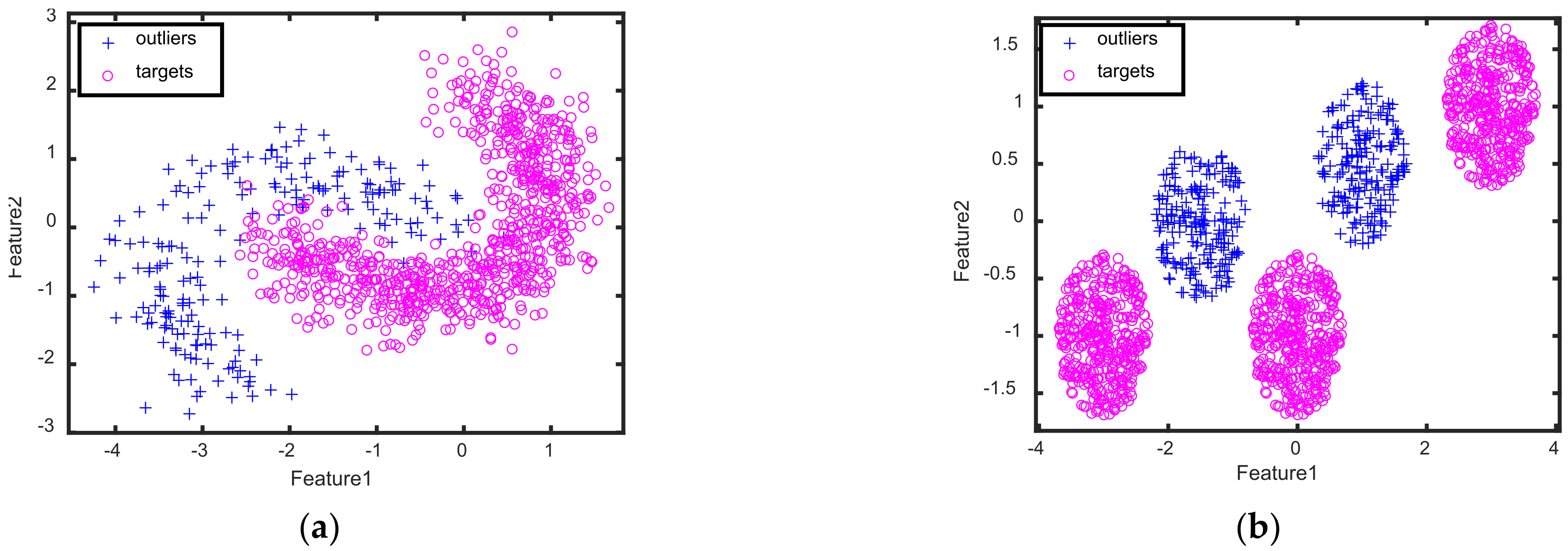
Two kinds of 2D toy datasets, including the banana-shaped dataset and Gaussian Mixture Model (GMM) dataset, are generated to show the visualization results of our method, in which the banana-shaped dataset is the single-mode datasets with both convex and concave edge regions, while the Gaussian Mixture Model (GMM) dataset is the multimode dataset. For the banana-shaped dataset, 400 samples are randomly sampled from a banana distribution to obtain the target samples, in which 200 samples are randomly chosen as the train target samples and the rest are used as the test target samples. Moreover, 200 samples are randomly sampled from other banana distributions to obtain the outliers in the test dataset. For the GMM dataset, 300 samples are randomly sampled from the GMM with each mode having 100 samples to respectively form the target samples in the training and test datasets, and 200 samples are sampled from other GMMs with each mode having 100 samples to form the outliers in the test dataset. Figure 3 presents the samples of targets and clutters for two kinds of 2D synthetic datasets, which shows that the distribution of targets are different from that of the outliers.

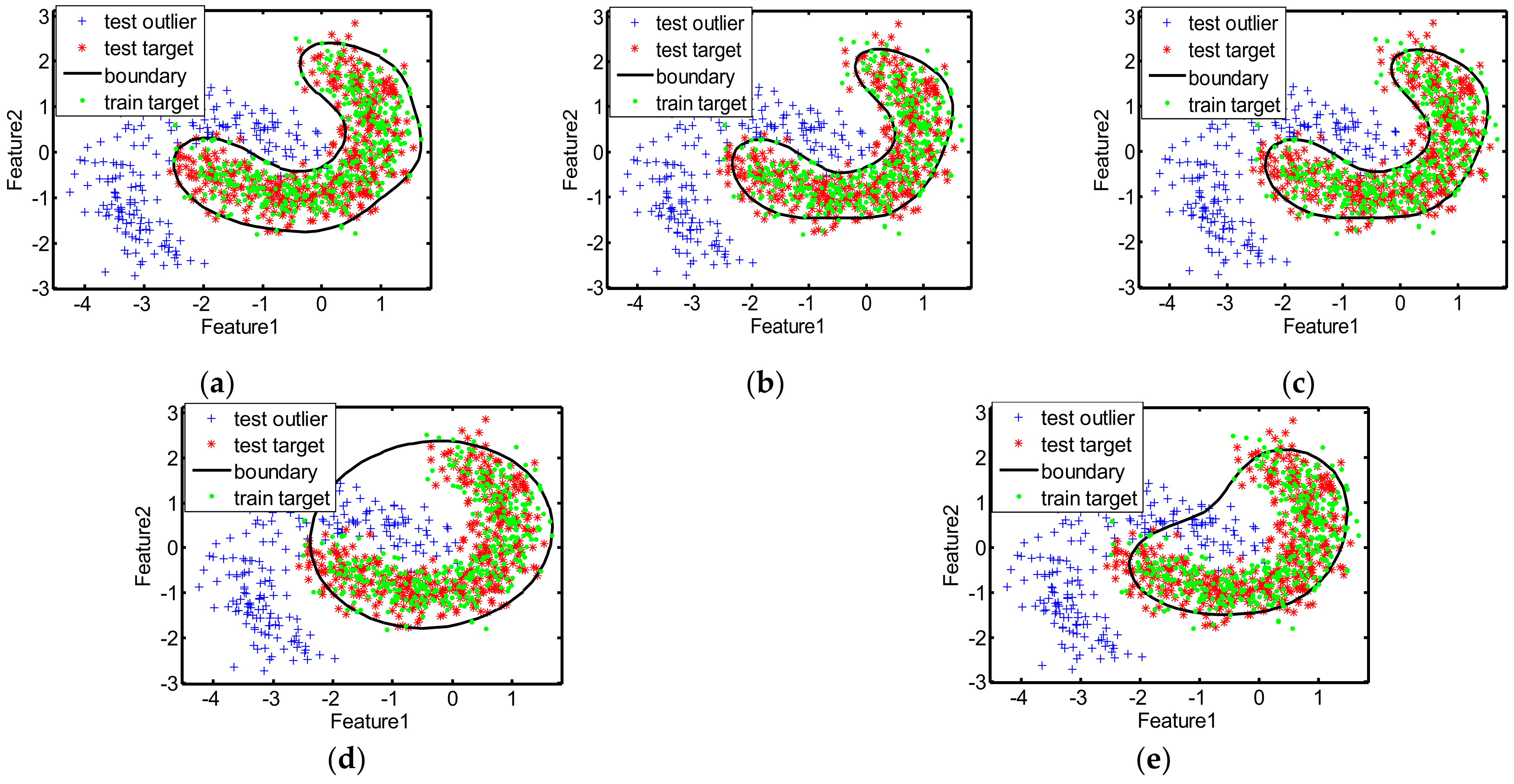
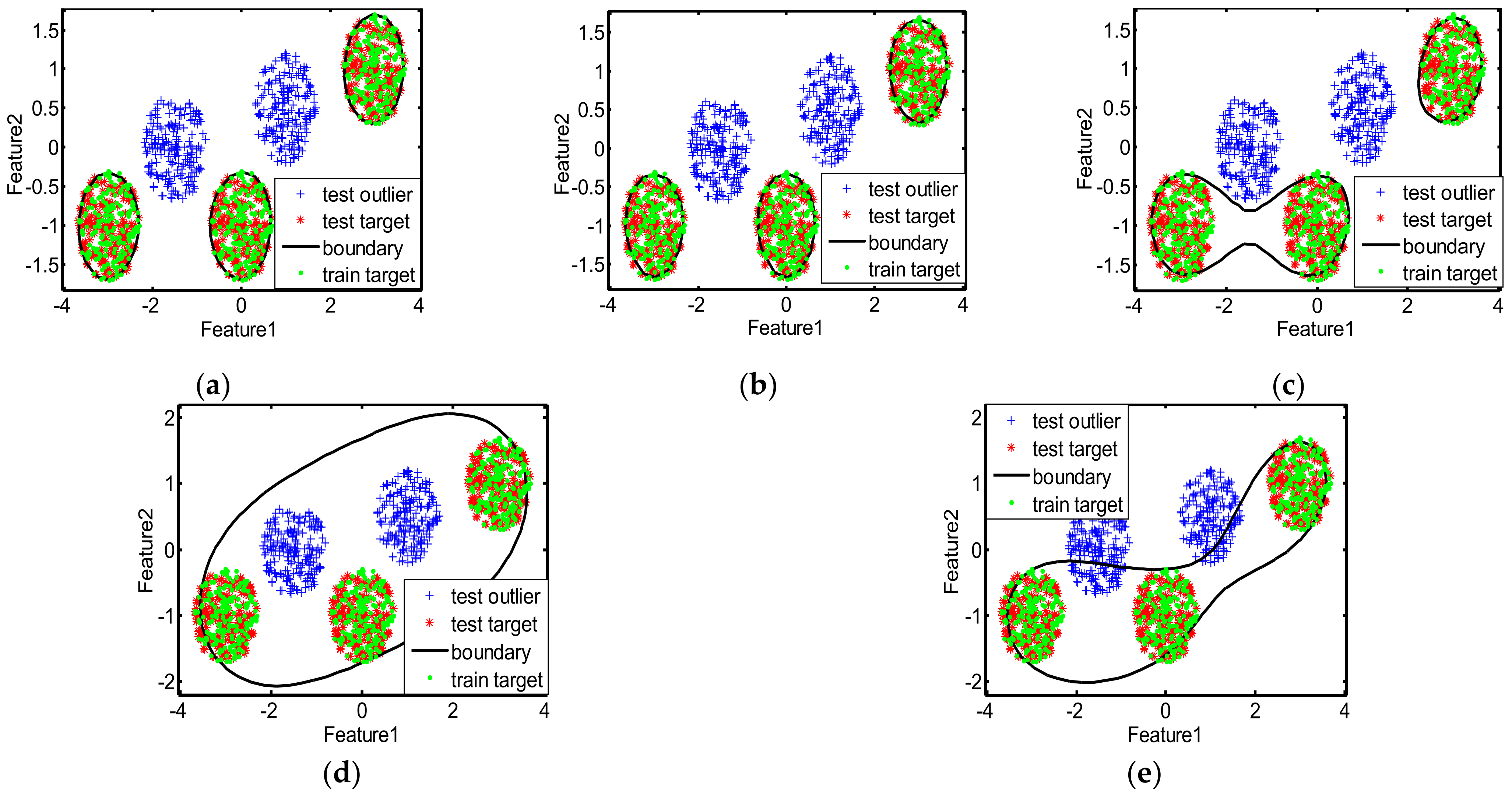
The decision boundaries learned by different methods for the two toy datasets are displayed in Figure 4 and Figure 5, and the corresponding quantitative classification results are presented in

Table 2. The classification results (%) of different methods on the banana-shaped dataset.

Methods	Precision	Recall	F1score	Accuracy	AUC
MIES	98.25	86.00	91.98	90.00	97.63
MinSV+MaxL	97.55	85.25	91.42	89.33	97.57
SKEW	83.00	92.00	88.16	83.17	71.72
MD	89.09	85.75	87.39	83.50	89.25
Our Method	98.41	92.75	95.50	94.17	98.76

and

Table 3. The classification results (%) of different methods on the GMMdataset.

Methods	Precision	Recall	F1score	Accuracy	AUC
MIES	100.00	86.17	91.70	92.57	99.98
MinSV+MaxL	100.00	95.47	97.68	94.80	99.94
SKEW	58.59	94.33	72.29	56.60	7.60
MD	82.83	87.67	85.18	81.70	89.62
Our Method	100.00	95.50	97.70	97.30	100.00

, where the red bold denotes the best values on each dataset, and the bold italic denotes the second-best results per column. As can be seen in Figure 4, the decision boundaries of MIES and MinSV+MaxL are a litter tighter than our method, and the targets outside the boundaries are greater in number, thus missing alarms are more numerous and the recalls are lower. However, the decision boundaries of MD and SKEW are much looser, with many outliers inside the boundaries, which devotes to more false alarms and lower precision. Moreover, as shown in Figure 5, for the GMM-shaped dataset, the decision boundaries of MinSV+MaxL, SKEW, and MD are loose, thus there are many false alarms leading to low precision. The quantitative results in Table 2 and Table 3 also indicate the better performance of our method than other methods on the toy datasets, with much higher precision, recall, F1score, accuracy, and AUC, since our method can learn the suitable kernel parameter that is utilized to obtain the decision boundary that is neither tight nor loose for the two toy datasets.

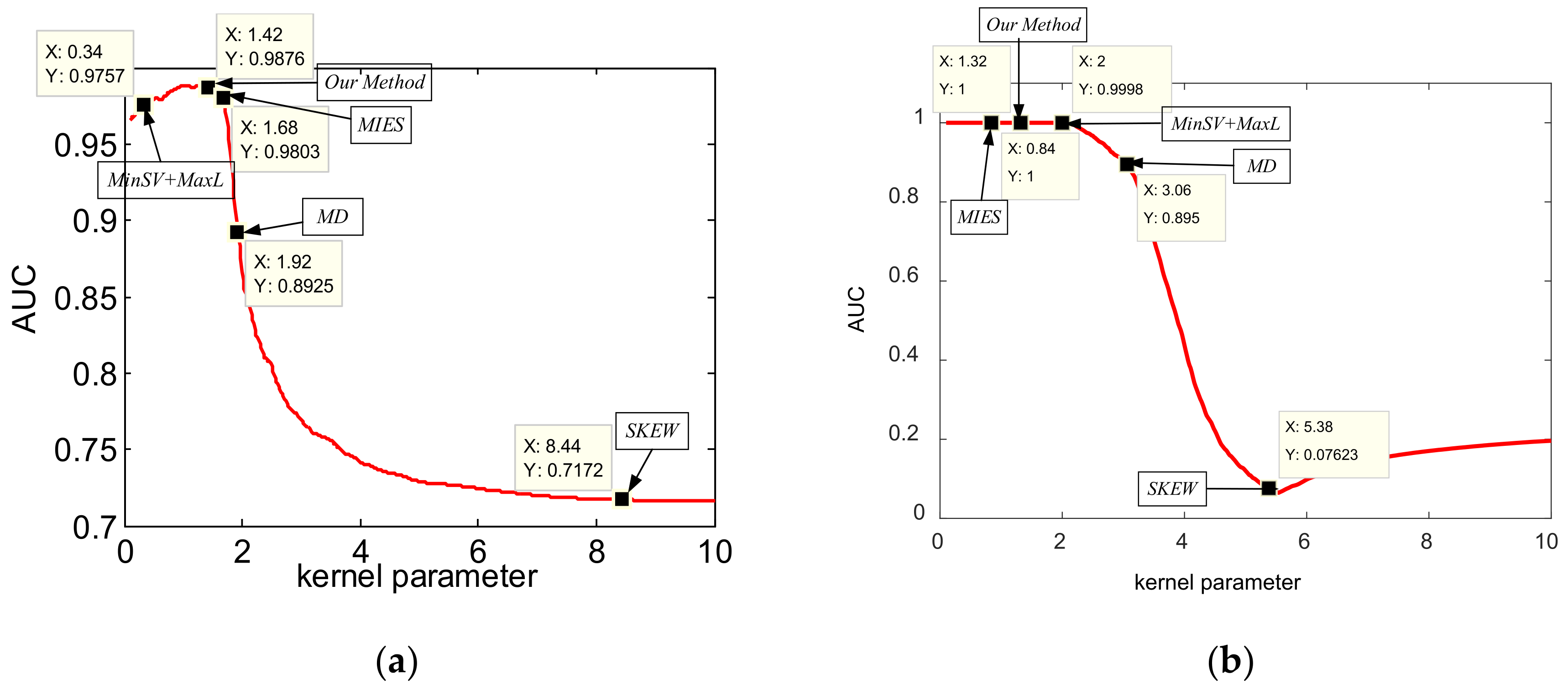
To further analyze the effectiveness of our method on learning the optimal kernel parameter, we present the test AUC curves with different kernel parameters, and point out the selected/learned kernel parameters by different methods in Figure 6. As we see from Figure 6, our method can learn the optimal kernel parameters on the curves, while other methods select the parameters either larger or smaller than the optimal solutions. Therefore, toy dataset results validate that our method can learn the optimal kernel parameter for the max-margin one-class classifier, which further helps it to learn the suitable decision boundaries to achieve the promising target discriminative performance.

4.2. Experiments on Measured SAR Dataset

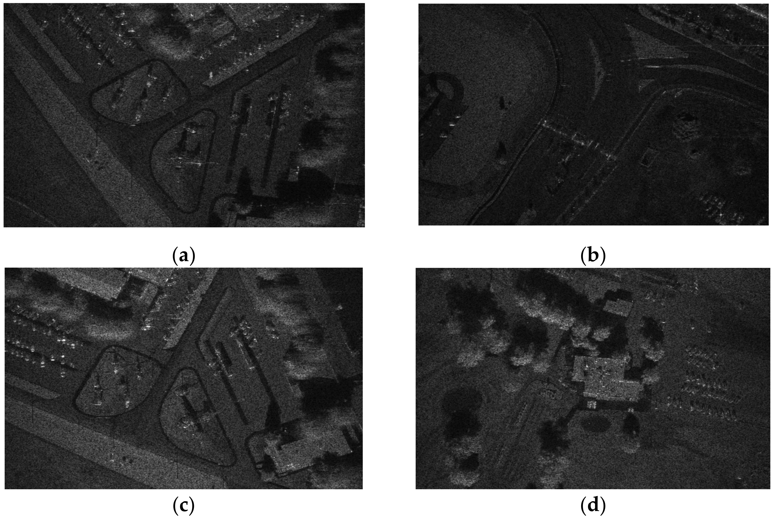
In the following, a measured SAR dataset is utilized to verify the effectiveness of our method. In the field of automatic target recognition (ATR), the OCC task for SAR images is usually referred to the SAR target discrimination. The measured SAR dataset we used here is the MiniSAR dataset [30,31,32], which was collected by the Sandia National Laboratories of America, Albuquerque, NM, USA, in 2005. Moreover, the resolution of the images in the MiniSAR dataset is 0.1 m, and their size is 1638 × 2501. The MiniSAR dataset contains 20 images, from which we choose 4 images: 3 images for training and 1 image for testing. In Figure 7, we present the chosen four images, and we can see that their scenes are very complex. There are numerous SAR targets in the four images, covering cars, trees, buildings, grasslands, concrete grounds, roads, vegetation, a golf course, baseball field, and so on. Among these SAR targets, the cars are the target of interest, and other targets are regarded as the clutters.

With the visual attention-based target detection algorithm [18], chips measuring 100 $\times$ 100 are obtained from SAR images of the MiniSAR dataset.

Table 4. The number of detected results for the 4 SAR images.

	Number of Total Chips	Number of Targets	Number of Clutters
Training dataset	250	135	115
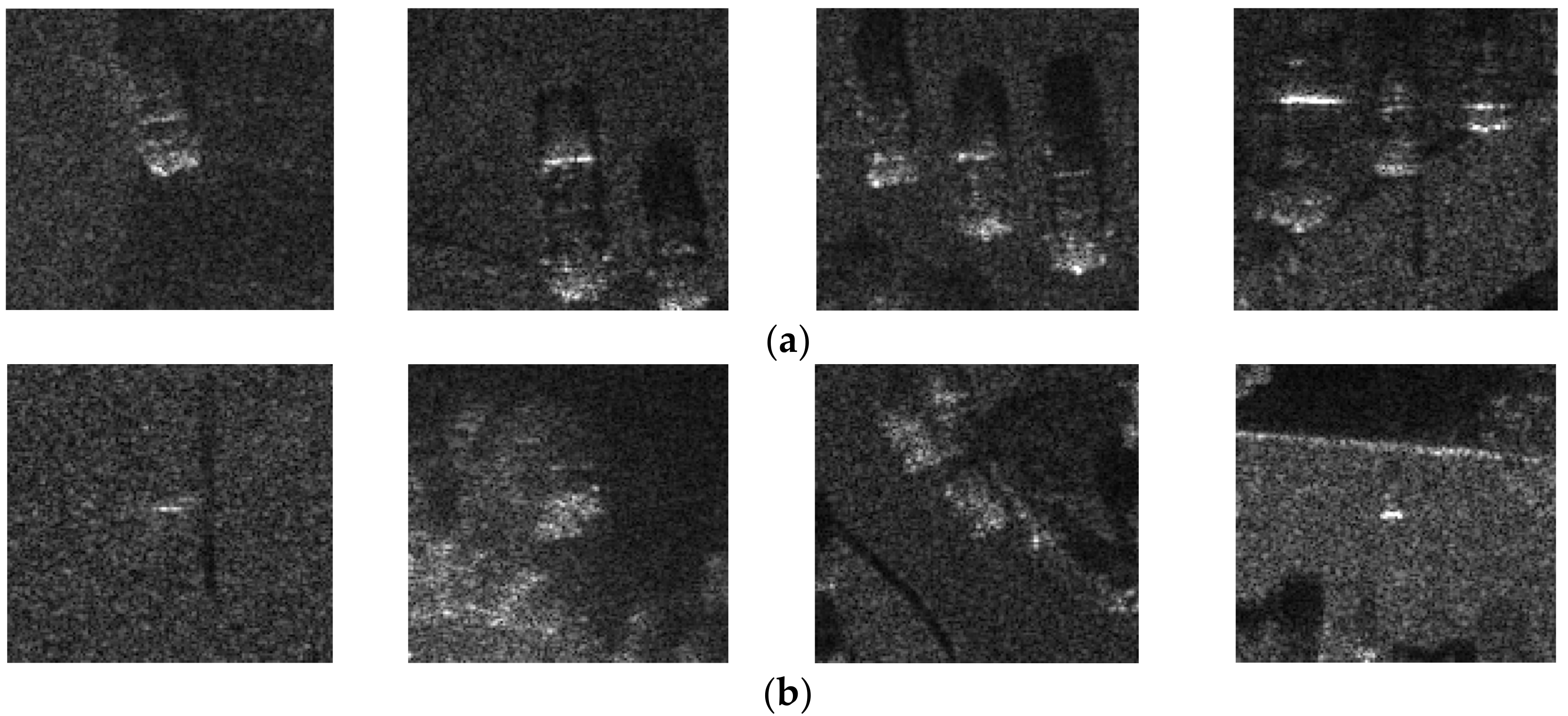
Test dataset	74	45	29

presents the detection results for the four SAR images in the MiniSAR data, and some chips from the MiniSAR dataset are given in Figure 8, where target samples are shown in the first row, and the clutter samples are shown in the second row. Since only target chips are used in the training stage, the training dataset only contains 135 target chips for the kernel parameter selection/learning methods.

First of all, we conduct the target discrimination experiments compared with some kernel parameter selection/learning methods for the max-margin one-class classifier to illustrate the better performance of our adaptive method. The values of precision, recall, F1score, accuracy, and AUC results for different parameter selection/learning methods for the MiniSAR dataset are listed in

Table 5. The test results (%) of different kernel parameter selection and optimization methods on MiniSAR dataset.

Methods	Precision	Recall	F1score	Accuracy	AUC
MIES	78.05	71.11	74.42	71.27	79.08
MinSV+MaxL	75.56	72.37	73.93	70.27	78.70
SKEW	71.23	70.58	70.90	39.19	75.94
MD	76.74	73.33	75.00	70.27	80.23
Our Method	86.84	73.43	79.52	77.03	83.07

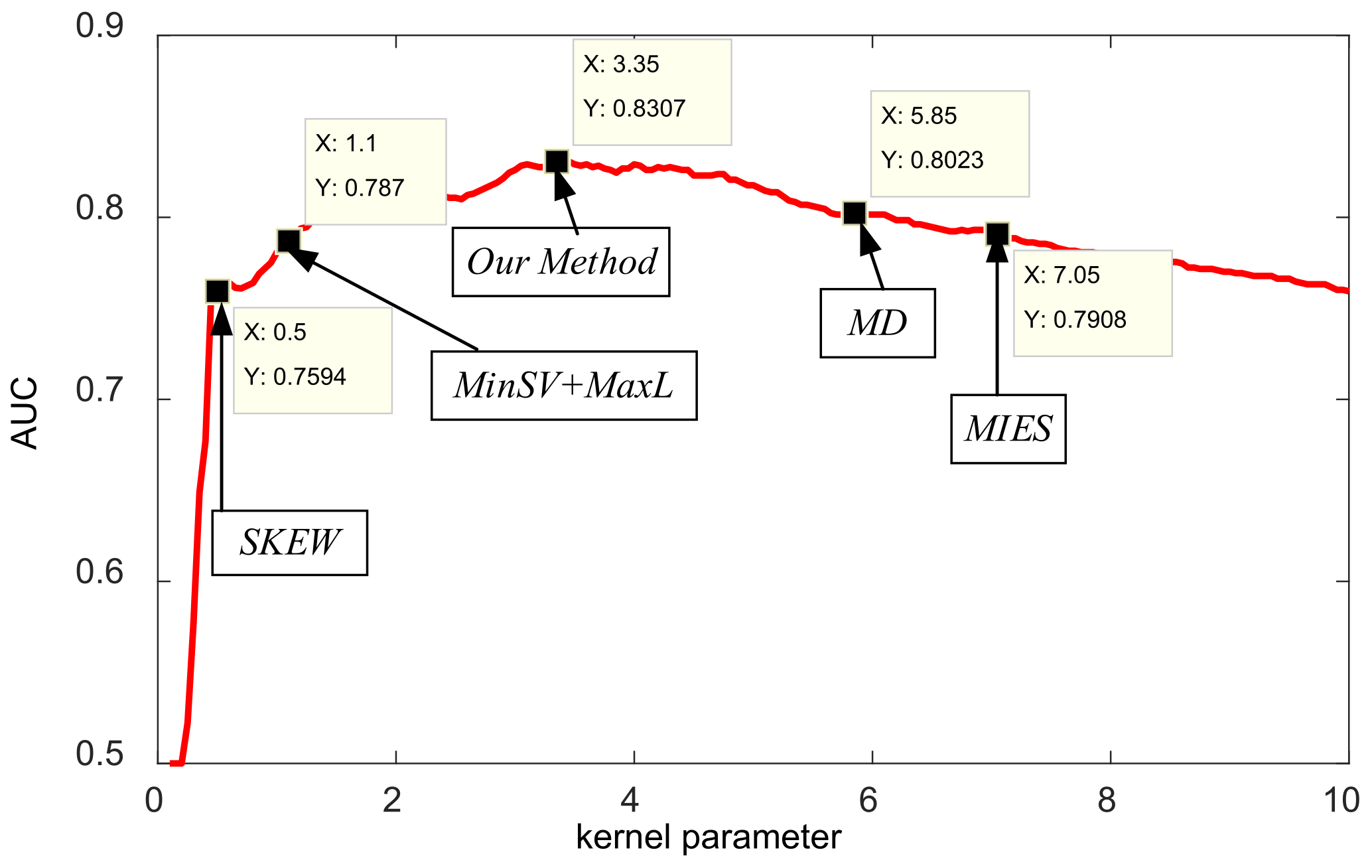
, where the red bold denotes the best values on each dataset, and the bold italic denotes the second-best results per column. In Table 5, it is obvious that the best results for the measured dataset are obtained by our method in all criteria, which indicates our method can achieve significantly less false alarms and missing alarms, and thus gain much higher precision, recall, F1score, accuracy, and AUC results. In addition, in Figure 9 we further plot the test AUC curves with different kernel parameters and indicate the selected or learned kernel parameters by different methods for the dataset, in which our method reaches the optimal values with maximum test AUC. Therefore, we can conclude that our method can learn the optimal kernel parameter for the MiniSAR dataset, which demonstrates the effectiveness of our method for target discrimination.

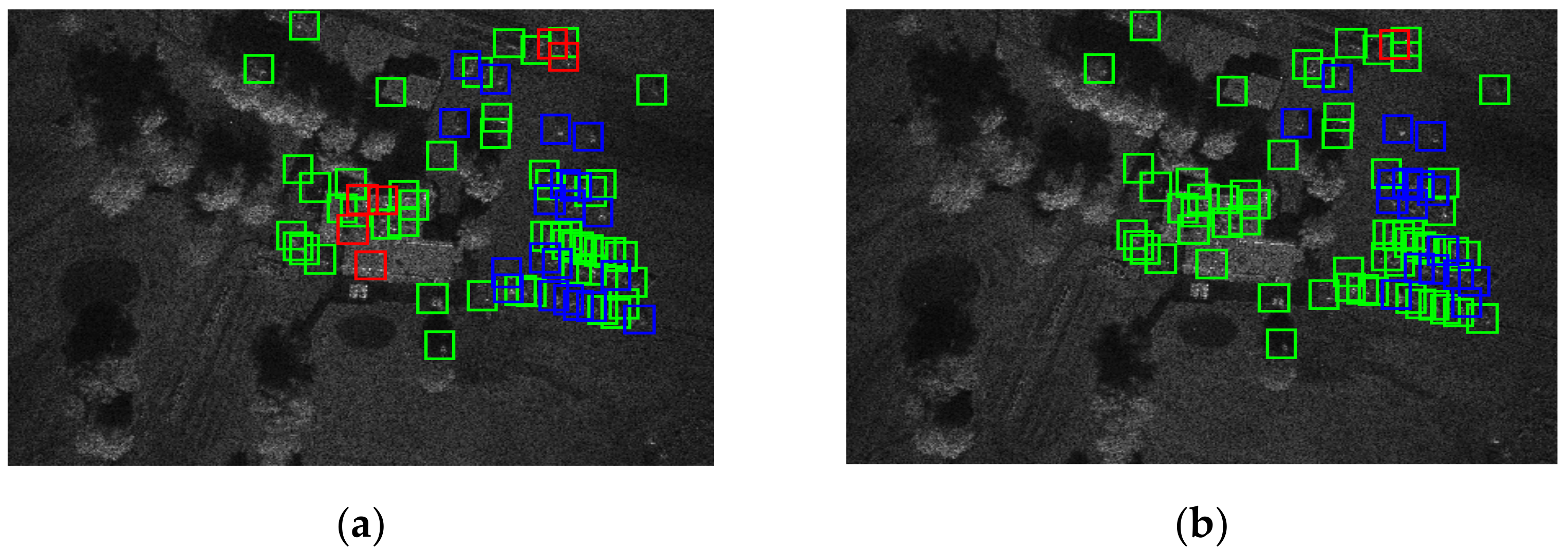
In SAR target discrimination, two-class SVM [29] is also a common discriminator. Therefore, the performance of our method is compared with the two-class SVM on the MiniSAR dataset. Figure 10 shows the visualization results of our method and two-class SVM on the test SAR image, where green boxes denote the chip correctly discriminated, blue boxes denote the target chip correctly discriminated, and red boxes denote the clutter chip wrongly discriminated. From the discrimination results in Figure 10, our method gains much less false alarms, less missing alarms, and more corrected targets, illustrating the better discrimination performance of our method than that of the two-class SVM.

To quantitatively compare the discrimination performance of our method with some other commonly used target discriminative methods,

Table 6. The test results (%) of different methods on the MiniSAR dataset.

Methods	Precision	Recall	F1score	Accuracy	AUC
k-means	41.38	93.33	57.33	67.36	75.10
PCA	34.38	93.33	50.24	63.91	69.27
Gauss	41.38	93.33	57.33	67.36	70.73
MST	31.34	91.11	46.63	61.07	71.57
SOM	44.83	93.33	60.56	69.08	74.79
AE	34.38	93.33	50.24	63.91	69.81
MPM	51.72	82.22	63.49	66.97	75.63
Two-class SVM	58.62	68.89	63.34	72.94	72.64
Our Method	86.84	73.43	79.57	77.03	83.07

lists the results of our method with some other discriminators. As shown in Table 6, the precision of our method is far higher than other methods, since the proposed method is a one-class classifier, while other methods are two-class methods that are trained with the targets and clutters. In complex SAR scenes, the SAR images contain multiple clutters. When the clutters in the training images are different from those in the test images, the performance of these methods will degrade a lot. Thus, these two-class classification methods tend to classify the background clutters as targets, and then the false alarms are very high, which leads to low precision. In addition, since these two-class classification methods learn the features of targets and clutters, most of the targets can be truly classified by these two-class classification methods, and then the number of false alarms FP is small, which further aids high recall. Since our method is trained only with target samples, it can effectively decrease false alarms and cause some missing alarms, which respectively leads to high precision and low recall. The F1score presents the harmonic mean between the precision and recall. According to other quantitative results in

Table 7. The learned values $l$ for an edge sample and an interior sample.

Samples	Edge Sample	Interior Sample
The learned values $l$	0.9355	0.5160

, our method performs well on the SAR dataset in complex scenes with much higher values of F1score, accuracy and AUC, which comprehensively illustrates the promising target discrimination performance of our method.

5. Discussion

5.1. Model Analysis

To visualize the effect of the algorithm of edge and interior samples selection in our method, we randomly choose an edge sample and an interior sample from the GMM dataset to present their k-nearest neighbors, normal vectors, and tangent planes. In Figure 11a, the near neighbors of the edge sample are mainly located on one side of its tangent plane, while Figure 11b shows that the near neighbors of the interior sample are well-distributed on the two sides of its tangent plane, which validates the theoretical local geometric relationship between the edge and interior samples with their nearest neighbors. Moreover, the values $l$ of the edge samples and interior samples are listed in Table 7, which are very close to 1 and 0.5, respectively. Therefore, the results in Figure 11 and Table 7 verify the effectiveness of the sample selecting algorithm.

Moreover, we also take the GMM dataset as an example to analyze the effect of samples selection on the learning of optimal kernel parameter and the boundary. Figure 12a–c shows the edge and interior samples selected by the algorithm in Section 3.1 with different parameters, in which red marks ‘$\ast$’ denote the interior samples, and black marks ‘$\square$’ denote the edge samples. From Figure 12a–c, we can see that the number of these selected samples gradually decreases. Moreover, in the three cases of selecting different numbers of samples, the corresponding curves of the objective function are presented in Figure 12d. As presented in Figure 12d, the respective maximums of the three objective function curves are reached when the kernel parameter equals the same values, i.e., $s^{\ast }=1.32$, which are marked with the red points. Moreover, in Figure 12a–c, the learned decision boundaries by our method are almost the same even though the number of selected edge samples and interior samples varies. Therefore, within a certain range, the objective function of our method is not very sensitive to the number of selected samples and can learn the optimal kernel parameter to build the suitable decision boundary.

In addition, we take the GMM dataset as an example to analyze the relationship between the distance from the samples to the boundary and the entropy values of samples. Under the optimal kernel parameter, we calculate the samples’ information entropy in the kernel space, and in Figure 13, we indicate the samples with M-maximum information entropy with a black mark ‘$\square$’ and N-minimum information entropy with a red mark ‘$\ast$’. As presented in Figure 13, the samples with large entropy values are located very close to the decision boundary, while the samples with small entropy values are mainly located in the center of Gaussian distributions that is far from the decision boundary. To sum up, Figure 13 shows that the larger entropy value a sample has, the closer the sample is to the boundary, which further validates the effectiveness of the defined information entropy for measuring the distance between a sample and the classification boundary.

5.2. Computational Complexity

Moreover, computational complexity is an important criterion with which to measure the practicality of a method. To analyze the computational complexity of our method with several one-class classification methods,

Table 8. The computational complexity and computation time (s) of different methods.

Methods	MIES	MinSV+MaxL	SKEW	MD	Our Method
Computational complexity	$O\left(M\left(N^3+N_{SV}^2+N_{SV}{N}_{IE}\right)\right)$	$O\left(M{N}^3\right)$	$O\left(M{N}^3\right)$	$O\left(N^2\right)$	$O\left(N^2+N_{Iter}{N}_{IE}N\right)$
Computation time (s)	36.58	9.20	10.16	0.53	0.76

presents the results. The computational complexity of the max-margin one-class classifier is $O\left(N^3\right)$ [9], and the computational complexity of SKEW and MinSV+MaxL is $O\left(M{N}^3\right)$, with $M$ denoting the number of elements in the kernel parameter candidate set and $N$ denoting the number of training samples. The computational complexity of MIES is given in [14], e.g., $O\left(M{N}^3+M{N}_{SV}^2+M{N}_{SV}{N}_{IE}\right)$, where $N_{SV}$ represents the number of support vectors, and $N_{IE}$ denotes the number of selected edge and interior samples. In [17], the computational complexity of MD is $O\left(N^2\right)$. In the first step of our method, the edge and interior samples are selected from the training set and the computational complexity of this step is $O\left(N^2\right)$. Then, in the second step, the entropy values for the edge and interior samples are calculated, and the computational complexity of this step is $O\left(N_{IE}N\right)$. Therefore, the computational complexity of our method is $O\left(N^2+N_{Iter}{N}_{IE}N\right)$, where $N_{Iter}$ denotes the number of iterations in gradient descent algorithm. Based on the above analysis, we list the computational complexity of different methods in the second row of Table 8. It is obvious that the computational complexity of our method is lower than those of MIES, MinSV+MaxL, and SKEW, and higher than that of MD.

Finally, the third row of Table 8 shows the computation time of the different kernel parameter selection/learning methods from the MiniSAR dataset. The red bold denotes the best values on each dataset, and the bold italic denotes the second-best results per column. It is obvious that the computation cost of our method is much less than those of MIES, MinSV+MaxL, and SKEW, and only a little more than that of MD. Although the computation burden of MD is smallest, there is almost no difference between the MD and our method, while the discrimination performance of MD is far lower than our method on used datasets. Therefore, on the consideration of computation cost and discrimination performance, our method can obtain the best discrimination results with a small computation burden compared with some parameter selection/learning one-class classification methods.

6. Conclusions

This paper focuses on the construction of a novel adaptive max-margin one-class classifier for SAR target discrimination in complex scenes. On the basis of the geometric relationship between the sample and classification boundary, we define the information entropy of samples in kernel space to measure the distance between a sample and the boundary. Thus, our method can automatically obtain the optimal kernel parameter of the max-margin one-class classifier, which is adaptive to SAR images with multiple clutters. The experiments on the synthetic datasets validate that our method is effective to learn the optimal kernel parameter of the max-margin one-class classifier, and then achieves the optimal target discrimination performance. Moreover, the experiments on the measured SAR dataset further verify the effectiveness of our method on SAR target discrimination in complex scenes. In addition, the analysis of computational complexity shows the promising practicality of our method.