An Improved L2Net for Repetitive Texture Image Registration with Intensity Difference Heterogeneous SAR Images

Abstract

Heterogeneous synthetic aperture radar (SAR) images contain more complementary information compared with homologous SAR images; thus, the comprehensive utilization of heterogeneous SAR images could potentially improve performance for the monitoring of sea surface objects, such as sea ice and enteromorpha. Image registration is key to the application of monitoring sea surface objects. Heterogeneous SAR images have intensity differences and resolution differences, and after the uniform resolution, intensity differences are one of the most important factors affecting the image registration accuracy. In addition, sea surface objects have numerous repetitive and confusing features for feature extraction, which also limits the image registration accuracy. In this paper, we propose an improved L2Net network for image registration with intensity differences and repetitive texture features, using sea ice as the research object. The deep learning network can capture feature correlations between image patch pairs, and can obtain the correct matching from a large number of features with repetitive texture. In the SAR image pair, four patches of different sizes centered on the corner points are proposed as inputs. Thus, local features and more global features are fused to obtain excellent structural features, to distinguish between different repetitive textural features, add contextual information, further improve the feature correlation, and improve the accuracy of image registration. An outlier removal strategy is proposed to remove false matches due to repetitive textures. Finally, the effectiveness of our method was verified by comparative experiments.

1. Introduction

Tasks such as environmental monitoring and change detection highly benefit from heterogeneous synthetic aperture radar (SAR) data, in short time intervals and high resolution, about an area of interest. A short interval is limited by a single spaceborne SAR sensor, owing to its long transit period. Therefore, it is becoming the trend to establish a short-time-interval image sequence for high-precision sea ice drift tracking. With the development of satellite technology, many types of SAR imagery, such as Advanced SAR(ASAR), Radarsat-2, European Remote Sensing1 SAR(ERS-1), and GAOFEN-3, provide us with the guarantee of heterogeneous imagery, which provides a tremendous database for civilian and military applications, such as land-cover and land-use analysis, and ocean monitoring [1,2,3,4,5,6,7,8].

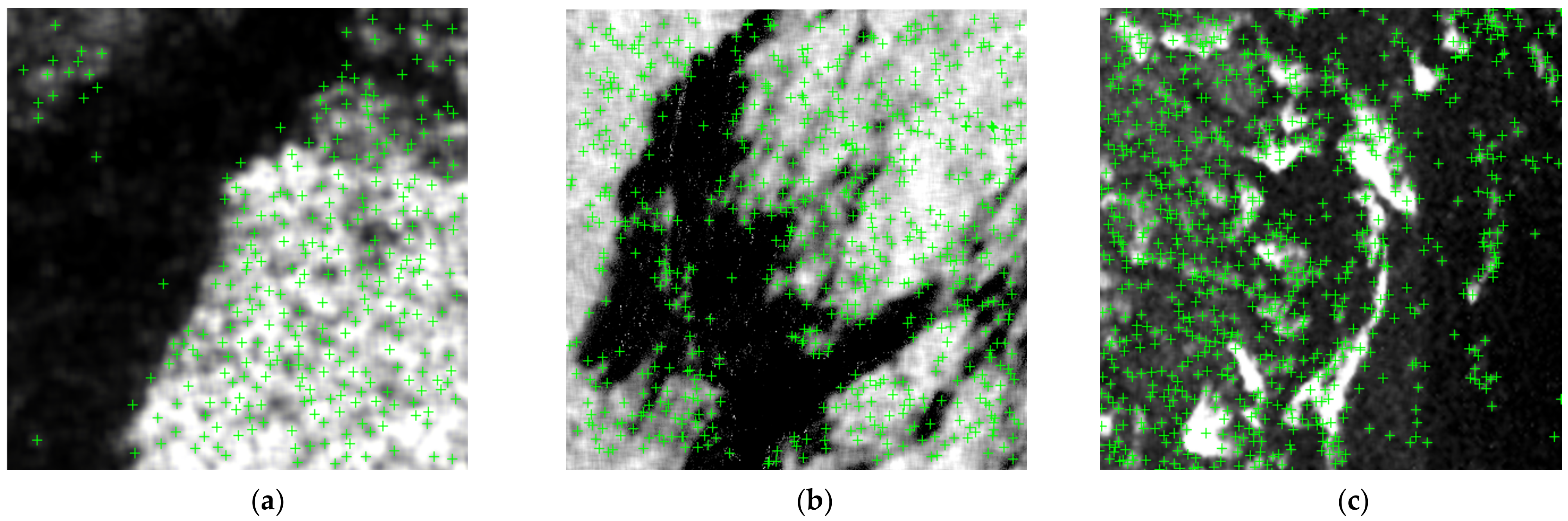
Heterogeneous SAR image registration is a critical step in a wide range of applications, including image fusion, change detection, environment monitoring, mapping sciences, and image mosaic. The differences in sensors and product modes of heterogeneous SAR lead to resolution differences and intensity differences in heterogeneous SAR images, and these differences lead to differences in the same object features, which affect the image registration accuracy. After uniform resolution of the heterogeneous SAR images, the intensity differences lead to differences in image texture features, which reduce the accuracy of image registration. Meanwhile, sea surface objects, such as sea ice (Figure 1a), oil spill (Figure 1b), and enteromorpha (Figure 1c), contain numerous repetitive textural features. After feature extraction (such as the SIFT), these data present the following phenomena:

(1)

The images can extract numerous feature points, and the small differences between these features result in a very high proportion of outliers, as shown in Figure 1.

(2)

The same objectives (sea ice, oil spill, and enteromorpha, etc.) contain numerous repetitive textures that are similar. These repetitive texture features have similar feature descriptions, which leads to obtaining numerous false matches in the matching process and makes it more difficult to remove outliers.

For such problems, there is a great challenge with traditional intensity-based and feature-based image registration algorithms. In this paper, the SAR data are history data with a relatively long time interval. The maximum time interval is 13 h. Compared with oil spills and enteromorpha, sea ice structure is more stable. Considering the possible usage prospects, sea ice were used as subjects for the experiment, and the effectiveness of the proposed improved L2Net network in heterogeneous SAR image registration was experimentally demonstrated by comparing with several other algorithms.

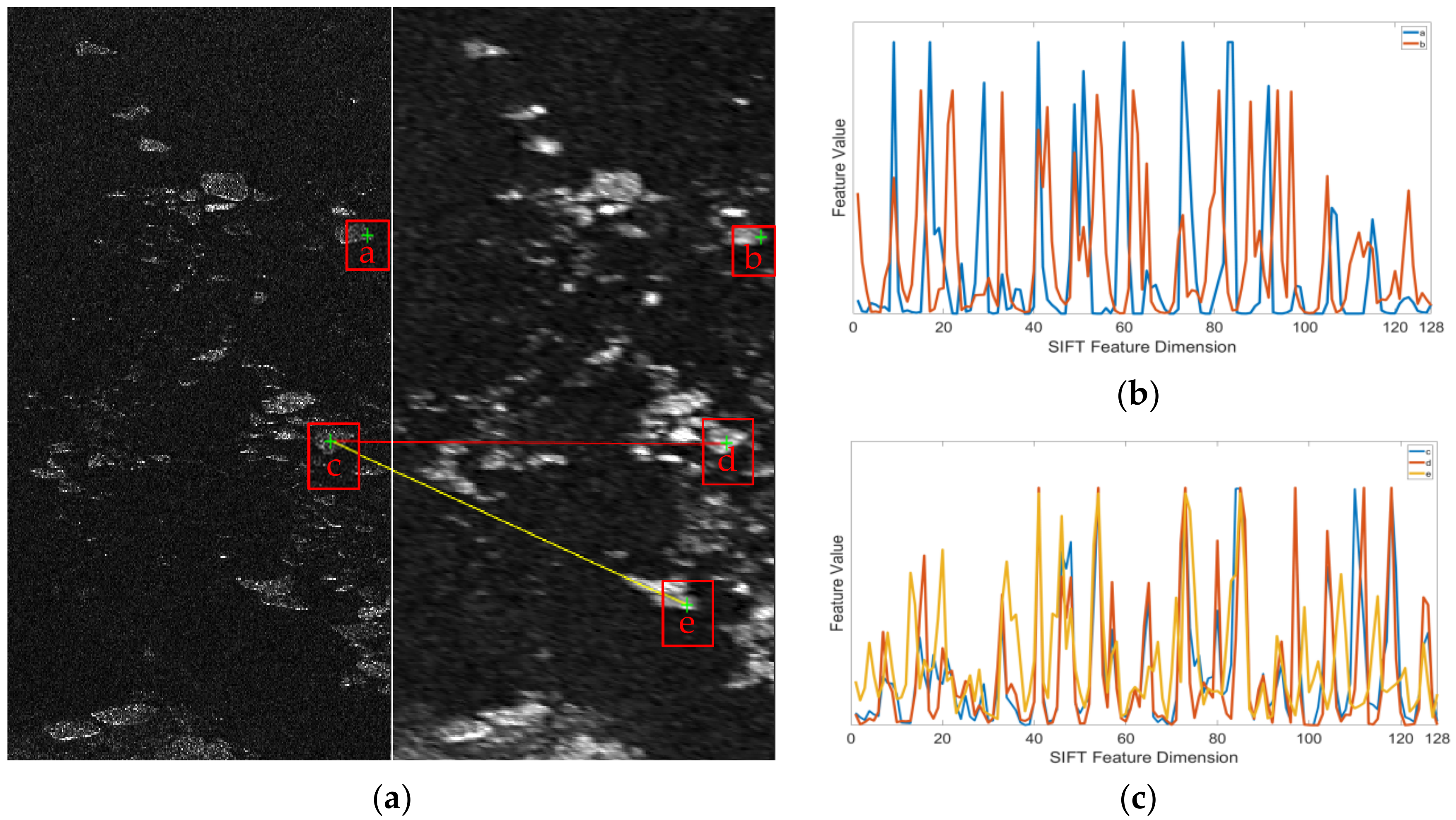
There is some inner connections between the non-homologous SAR images, but there are still differences from the surface, as shown in Figure 2a. The same sea surface objective in non-homologous SAR images has differences in its intensity, due to different sensors or product modes, so this means the final two features cannot be matched; for example, the sea ice is dark in the image at point a in Figure 2a, while the same sea ice is light in point b, and the descriptors extracted using the classical feature algorithm (SIFT) are also different, as shown in Figure 2b. It is obvious that a direct comparison using the classical algorithm will miss many matches. Therefore, it is crucial to reveal the inner relationship between the given image patch pairs. There are also numerous repetitive texture features on the sea surface objectives, and this will lead to multiple point matches for the same point, which further increases the difficulty of image feature registration. For example, in Figure 2a, the sea ice textures in the two boxes of point d and point e are similar, resulting in point c matching point e. The descriptors extracted using sift for the three points c, d, and e are similar, as shown in Figure 2c. Although the sea ice will drift, the motion of the sea ice follows the marine kinematics and will remain relatively consistent with the surrounding sea ice motion. By looking at the sea ice around point c and point e, it can be visualized that the sea ice at point c and point e are not the same piece of sea ice. They are false matches. Therefore, it is important to avoid the case of matching point c and point e. We found that the sea ice texture features in the image frames are similar, but the surrounding sea ice structure is different; thus, adding contextual features will improve the feature discrimination. Therefore, it is necessary to use deep learning methods to establish inner connections between image pairs and to use contextual relationships to enhance the correlation between image pairs and to increase the differentiation between features with a repetitive texture.

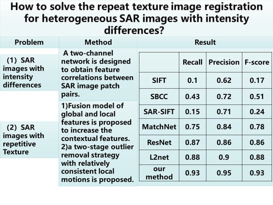
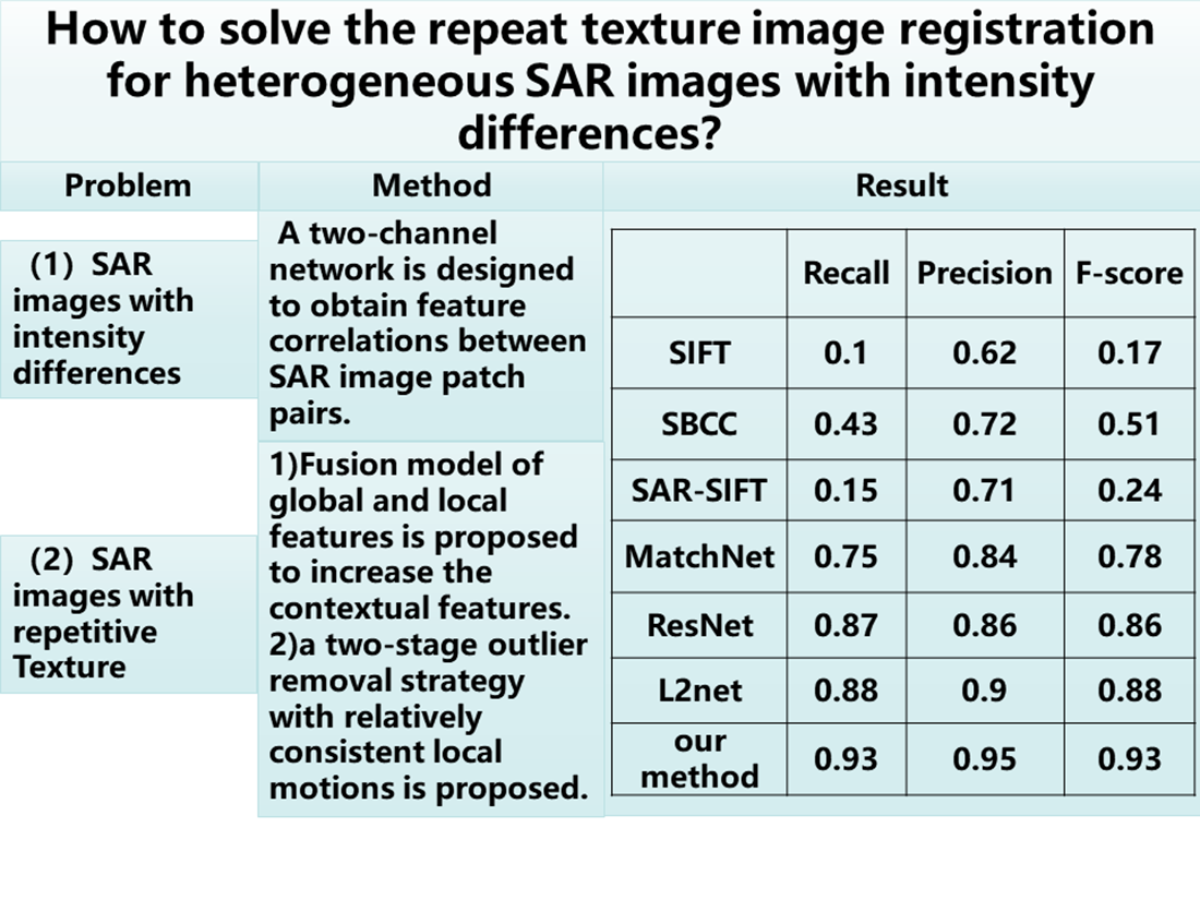
In this paper, based on the above-mentioned problems with sea ice as the object of study, we propose an improved L2Net network for solving the problem of feature matching with repetitive texture objects for short time intervals of heterogeneous imagery with intensity differences. The contributions of our proposed method are as follows:

(1)

A two-channel network is designed to obtain feature correlations between SAR image patch pairs. Compared with L2Net, every output feature of each branch, which contain two channels, is a multi-channel 2D feature, which can reinforce the feature correlations of SAR image intensity differences. To obtain more detailed features, the L2Net network structure is adjusted to reduce the pooling layer, while adding a feature fusion layer to strengthen the correlation between intensity difference images.

(2)

A fusion model of global and local features after the feature extraction layer is proposed, to increase the contextual features, which improves the descriptor discrimination of the repetitive texture feature.

(3)

Based on marine kinematics, we propose a two-stage outlier removal strategy, with relatively consistent local motions.

The rest of this paper is organized as follows. Section 2 discusses the background related work. Section 3 details our proposed method. The data used in the study and the experimental results are described in Section 4. Discussion is given in Section 5. Conclusions are given in Section 6.

2. Related Work

For the feature extraction task of homogeneous data, the selection of features has changed from the early manual selection, to the automatic selection of feature points.

The common methods of image registration can be divided into intensity-based methods and feature-based methods. Intensity-based methods calculate the intensity information of image pairs to compare the similarity. Feature-based matching methods are used to obtain matching information by calculating the special feature (point, line) matrix of the image, to compare the similarity. The common feature-based SAR image registration methods include scale-invariant feature transform (SIFT), oriented FAST and rotated BRIEF (ORB) features, and KAZE features. In 2004, Lowe [9] proposed and improved the SIFT feature, which is invariant to rotation, scale transformation, and brightness difference, and is widely used in image registration fields. A feature description algorithm, the ORB algorithm, was proposed by Rublee [10] and uses the FAST algorithm when selecting feature points, and uses BRIEF as a descriptor to describe the feature points. Muckenhuber [11] applied the ORB algorithm for the first time when tracking the sea ice of the Fram Strait and in the ice-covered waters north of Svalbard, and achieved good results. Demchev [12] applied the KAZE feature to sea ice drift tracking research. KAZE features are improved with nonlinear scale space to reduce the image information loss in response to the information loss that occurs in the linear scale space transformation of SIFT features. A straightforward block cross-correlation (SBCC) method was proposed for ice drift [13]. Compared with the obvious edge features of ground objects, sea ice features are fuzzy, and common feature descriptors are not effective in matching sea ice and sea ice features.

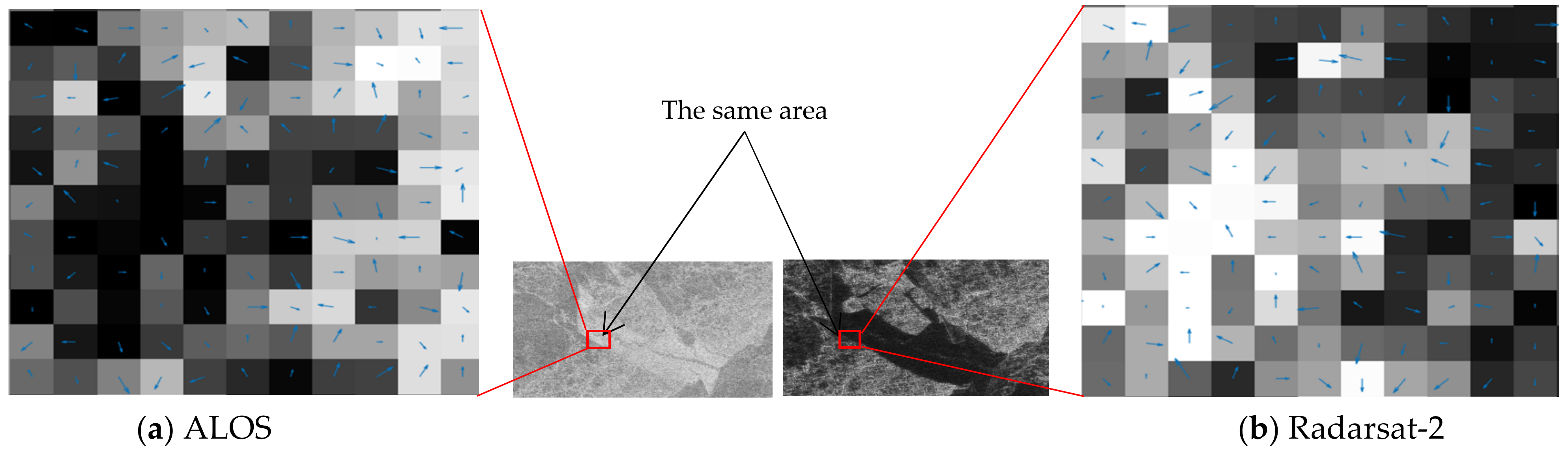
With the development of satellite technology, SAR imagery is becoming more available. However, there are differences in the sensor band, polarization mode, resolution, incident angle, and noise level of the sensors of different SAR satellites, resulting in significant feature differences between heterogeneous SAR images. Dierking [14] used 2D-PDF to study the sea ice correspondence between Radarsat-2 data and TerraSAR-X data and found that there was a high degree of similarity in sea ice, but not a one-to-one correspondence. Moreover the incidence angle of heterogeneous satellites, and the polarization mode can lead to radiation variations, which can cause large differences in the intensity of remote sensing images from different sensors. Figure 3 shows the same ice conditions from Radarsat-2 and ALOS, as well as the gradient calculation. From the figure, it can be seen that different satellite sensors lead to significant differences in the intensity of the images, resulting in large differences in the direction and magnitude of the gradients between the image pairs. The commonly used methods in sea ice tracking (SIFT, KAZE) use image intensity information and image gradient information in the calculation of image feature descriptors, and the intensity difference of data will lead to an inconsistent gradient direction when extracting similar feature points with two datasets in SIFT, KAZE, and other common methods for sea ice drift. The inconsistent main direction of feature descriptors leads to a low correlation of feature descriptors, and many false matches may, thus, occur when common feature descriptors are used for matching. Therefore, many mismatches will occur when using common feature descriptors for matching. Common feature descriptors have a limited ability to distinguish sea ice features from heterogeneous SAR images, and the matching effect is poor for such features, resulting in large errors in the results. In order to overcome the problem of the poor discrimination ability of SIFT in data with intensity differences in images, the angle of the SIFT calculation gradient can be changed from 360° to 180°, and all gradient directions exceeding 180° can be normalized to within 180°, which can improve the discrimination ability of the algorithm in this type of problem [15,16]. These methods have all been used in sea ice tracking research with homologous data, to obtain satisfactory results. However, the differences between heterogeneous imagery do not all vary linearly, leading to more mismatches when these methods perform heterogeneous image matching.

Many scholars have applied machine learning to image feature matching and have obtained many results. Deep learning networks have been widely used in a variety of remote sensing applications, including image segmentation [17,18,19,20] and image registration [21,22,23,24]. A convolutional neural network (CNN) based on pixel texture features can better extract image features [25,26]. However, when there are large discrepancies in images, there are large errors in extracting textural features by pixel-based machine learning of images. The Siamese network was proposed to solve the image registration problem with large differences between image pairs. This network is the dominant architecture of CNN based on descriptor learning [27,28,29]. To improve performance, a fully connected layer is favored by many researchers as a measurement network. Ronneberger [30] proposed a convolutional neural network named U-Net for image segmentation. ResUNet [31] replaces each sub-module of U-Net with a form of residual connections. MatchNet [32] is a typical Siamese network, which consists of a feature network that extracts feature representation, a bottleneck layer for dimensionality reduction, and a decision network that measures the similarity of feature pairs. This has been shown to significantly improve upon previous results and has the great potential of a CNN for descriptor learning. However, this method is limited by the network and requires more image training. Some scholars have proposed removing the metric learning layer, to make the network more flexible. As most matching networks require neural networks to extract image features, many Siamese networks aim to learn high-performance feature descriptors without metric networks. For example, the networks in [33,34,35] are common metric-free networks for Siamese networks. These Siamese networks are composed of two branches of deep learning networks that share weights and use the Euclidean distance as the loss function. They extract image feature descriptors by training a deep convolutional model and obtain image patch matching using the Euclidean distance. Due to the problem that the sea surface objectives have repetitive textural features, the above deep learning methods will extract numerous similar texture features, which leads to numerous false matches and affects the accuracy of matching. L2Net [36] uses the center and edge blocks to learn image features, and a high-performance feature description is obtained. This method uses the raw patch to intercept the central area and resamples to obtain a patch of the same size as the input; however, this method is not suitable for SAR images with a large amount of speckle noise and some fuzzy texture features, because the upsampling method will amplify the raw noise points, resulting in the reduced feature extraction vector recognition ability of the feature network. Therefore, L2Net cannot be applied to the feature matching problem of sea surface objectives in SAR images.

Through the feature correspondence analysis of an image, we propose an improved L2Net network method. To achieve image registration for heterogeneous SAR images with large intensity differences, we use a uniformly distributed feature point algorithm to obtain control points, and the image patches obtained at the center of a key point complete feature matching in our method.

3. Methodology

In this paper, we propose an improved L2Net network for image registration with intensity differences and repetitive textural features. Our method contains three steps: Step 1 involves input and pre-processing. In this step, the original images are filtered and geometrically calibrated. The algorithm in [37] is used to extract the control points and obtain the image patches as the network input. In the second step, the feature vectors are obtained by extracting the regional features using the Siamese-like neural network proposed in this paper. The similarity between the image patches is calculated in Step 3, for rough matching. Finally, based on marine kinematics, a removal outlier stage is proposed, to remove the incorrect matches and produce the final results. The details of each step will be presented in the following subsections.

3.1. Acquisition of Control Points

Image registration using deep learning network methods often uses the slider method to obtain patches for matching. The process of image matching using the slider approach is that a patch from one remote sensing image needs to match the whole image of another remote sensing image by sliding the window to find the matching patch, which usually increases the computational burden. Meanwhile, the size of the SAR image is large, and the use of the slider method for matching greatly reduces the efficiency of the algorithm. Therefore, we use the advantage of selecting the control point location first, which can effectively reduce the computation and improve the efficiency of the model by using the obvious features of the control points.

Classical control point selection methods, such as SIFT, ORB, and KAZE, obtain a nonuniform distribution of control points, and the distribution often appears to be aggregated, which will result in sampling to obtain image patches with overlapping areas. Image patches with overlapping regions produce a higher similarity of the features extracted by the network, which can increase the matching difficulty and reduce matching accuracy. Therefore, they are not suitable for selecting the location of sea ice control points. Komarov [37] proposed a novel feature point selection algorithm, which is based on the variance matrix of the image and can obtain uniformly distributed and more obvious feature points in the image. He used it for the selection of sea ice SAR image control points. The control points in the image were used for homologous sequence image matching. The proposed algorithm was applied to obtain more uniformly distributed control points for sea ice feature matching of a heterogeneous SAR image. This method was used to select the control points in this paper.

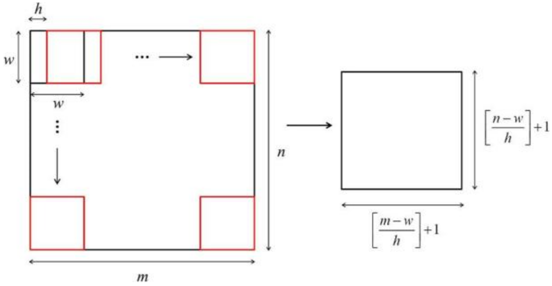
The control points were obtained by calculating the variance matrix, which is shown in Figure 4, following three filtering steps.

Calculate the variance matrix: as shown in Figure 4, each element of the variance matrix S1 is calculated from the window w × w, as follows:

$$\nu =\frac{1}{w^2}{\displaystyle \sum _{i,j=1}^w{(a_{ij}-\overline{a})}^2}$$

(1)

where w is the window size, $a_{ij}$ is the pixel value in the window, and $\overline{a}$ is the average pixel value within the window. The generated variance matrix is used as input for the control point selection.

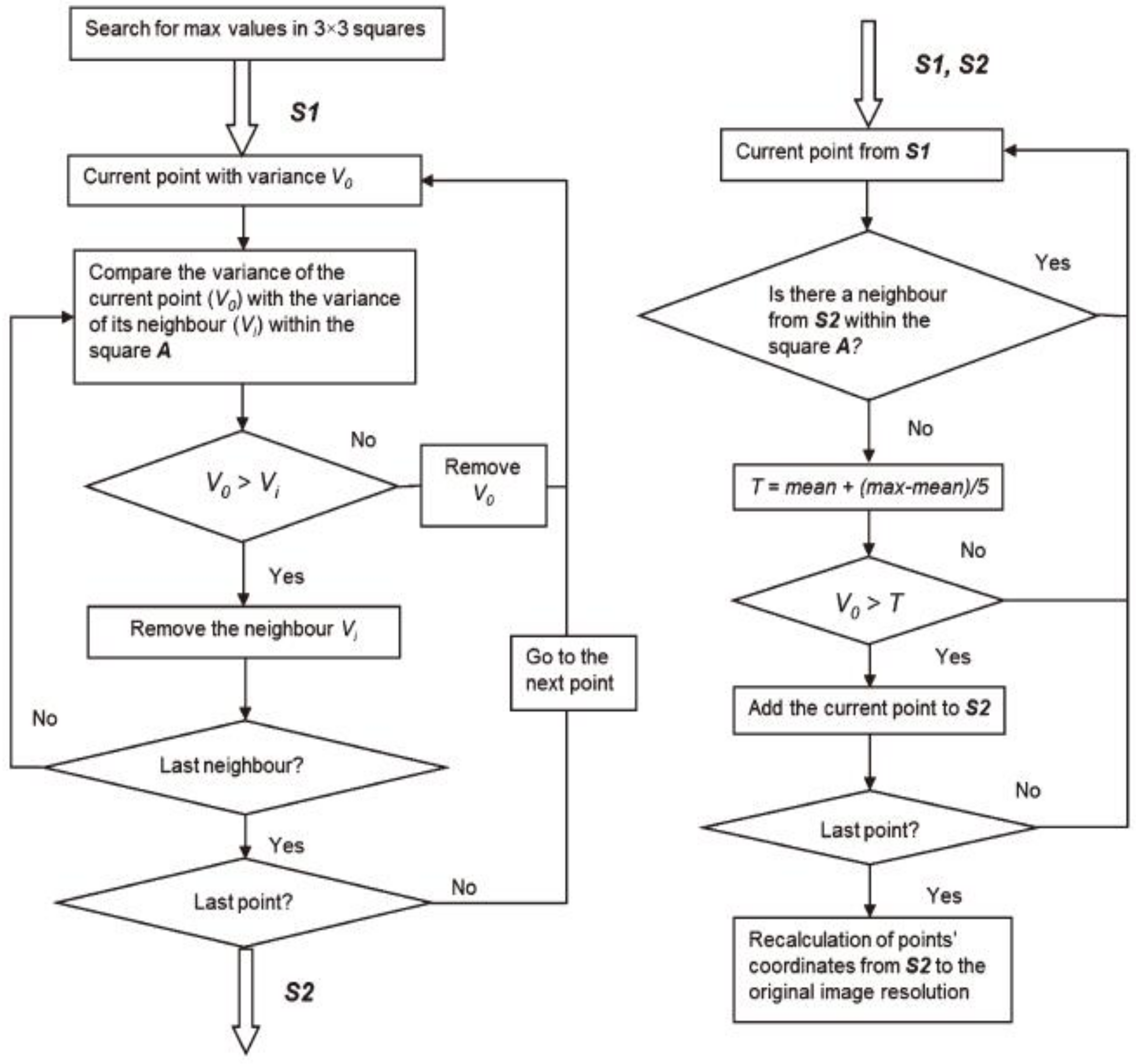
A selection of control points flowchart is shown in Figure 5. The first step is the initial screening of the elements in the variance matrix S1. The second traversal defines the local maxima in the surrounding (2R + 1) region (A), where R is a predefined parameter. The third round adds squared-off points for these regions where no maxima exist. A relatively uniform distribution of control points is finally obtained.

3.2. Image Matching Network Structure

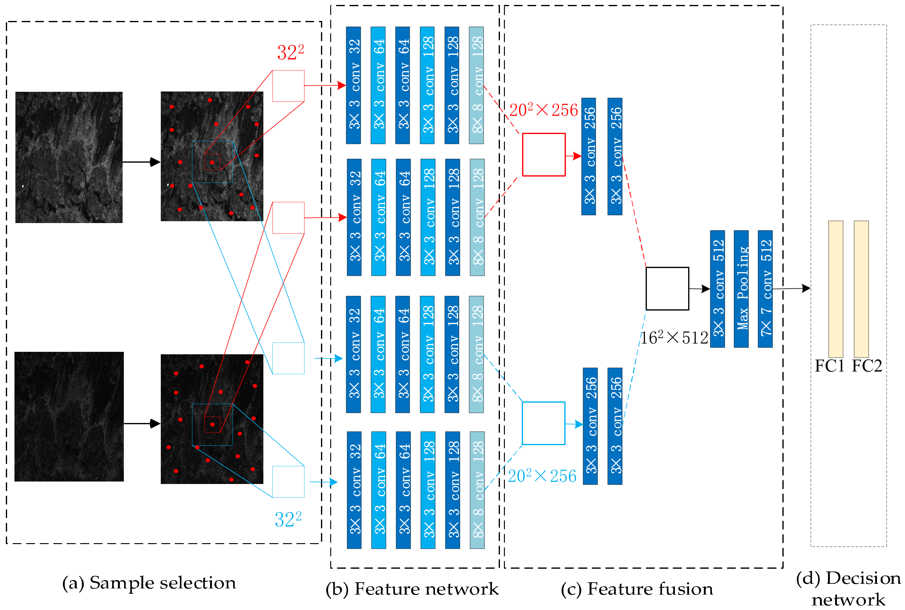
Using the slider approach to perform matching increases the computational burden. Image patches with texture features are obtained through control points and used as input for the network, which improves the efficiency of matching image features compared to the slider approach. This section will use the control points obtained in the previous section as the center, to obtain the image patches as the input of the network. The network architecture is shown in Figure 6.

3.2.1. Feature Network

Many scholars have used the CNN-based Siamese network for multi-mode image registration. However, the difference in non-linear gray scale results in a poor image matching accuracy. The Siamese network has only two image patch input feature extraction networks to extract the feature information of the image block. The texture structure between different sea ice image patches in sea ice SAR images may have similar textural structures, which will decrease the accuracy of the image patch matching. We propose a novel network structure inspired by L2Net algorithm, for the sea ice heterogeneous SAR image feature matching network.

L2Net takes a 32 × 32 image patch as input, and outputs a 128-dimension feature vector. In addition, a 32 × 32 patch input is implemented as a central-surround, and the input of one branch is the raw patch size. The input of the other branch is a small patch crop in the middle of the raw patch, and this small patch is upsampled to 32 × 32 size. Then, through the same network, the two network feature vectors are fused, and one feature vector is obtained.

L2Net uses the raw patch to intercept the central area and resamples to obtain the patch of the same size as the input; however, this method is not suitable for SAR images with a large amount of speckle noise and some fuzzy texture features, because the upsampling method will amplify the raw noise points, resulting in a reduced feature extraction vector recognition ability of the feature network. Moreover, remote sensing image patches usually contain numerous similar targets, whose image features are very similar, and using the input of L2Net will result in a fixed range of neighborhood information that may not be able to learn robust and discriminative feature representatives for all samples.

To solve the above problem, we proposed a new input for the network structure and also modified the network structure. There is a feature similarity problem between the small image patches of the same data; therefore, four image patches are used as input. For each image, we extract small patches with the raw resolution of n × n pixels. To improve the receptive field of the network, we additionally extract a small block of 2n × 2n pixels and downsample it to n × n pixel. In this way, local features and more global features are fused to obtain structural information, to effectively distinguish between sea ice and to add contextual information. Although downsampling will cause the loss of some textural feature information, more structural and contextual information is maintained. Image downsampling can also ensure a limited impact on memory consumption and computational overheads. Similar multi-scale methods have proven to be effective [38]. Thus, we have four image patches as input.

Our basic architecture is similar to L2Net, with seven convolutional layers. Each of these seven layers has the following number of filters: 32, 32, 64, 64, 128, 128, and 128. Furthermore, the two branches are trained independently, and the weights are not shared, to ensure that the two branches do not affect each other. The difference is that we set the stride value of each convolutional layer to 1, to prevent loss of spatial accuracy. At the same time, unlike most learned or hand-made features, the output feature of each branch is not a 1D vector 1×n vector, but a multi-channel 2D feature (k × k) × n.

Our proposed feature fusion module (as shown in Figure 6) consists of two feature fusions stages:

(1)

The first fusion stage is the fusion of two channel of features from the same branch, and contains two consecutive convolutional layers. The convolutional layers consist of 3 × 3 filters, which operate over the concatenated feature maps of the SAR. This is due to the fact that the fusion layer uses 3 × 3 convolutions to learn relationships between the features, while preserving nearby spatial information. Max pooling is omitted after the first convolutional layer in the first fusion stage. The maximum pooling layer is not used, in order to maintain the learning space relationship.

(2)

The second fusion stage is used to fuse the global features with the local features. Using a 3 × 3 convolution layer and max pooling layers, a 1 × 512 dimensional feature vector is finally obtained, with a 7 × 7 convolution. The final decision network consists of two fully connected layers: the first of which contains 512 channels; while the second contains 2 channels.

3.2.2. Loss Function

The Siamese-like network has different parameters, giving it more flexibility to extract the features according to the specificity. Now, we introduce the overall learning goals of the network. The datasets composed of image patch pairs with the label is defined as:${\{x_i^r,x_i^s,y_i\}}_{i=1}^N$, where N is the number of pairwise image patches. Although we use the structure of L2Net, its loss function cannot be applied to our feature vector and metric network. Therefore, the loss function is defined as the binary cross-entropy loss for our network:

$$E=\frac{1}{n}{\displaystyle \sum _{i=1}^N[y_i\log ({\widehat{\mathrm{y}}}_i)+(1-y_i)\log (1-{\widehat{\mathrm{y}}}_i)}]$$

(2)

where n stands for the number of input pairs, y_i is the label for the ith input pair, and this is a rough 0/1 label, while ${\widehat{\mathrm{y}}}_i$ is the corresponding matching probability when comparing the input pair $(x_i^r,x_i^s)$.

3.3. Outlier Removal

For a patch in the reference image, there may be some close neighborhood candidate patches in the sensing image. These candidate patches may have similar image information, and all corresponding matching probabilities are greater than 0.5. In addition, there are numerous repetitive features in the image patches, and the convolution operation in the network will contaminate the edge information of the samples; and although the matching accuracy can be improved by adding contextual information, there will still be some error matches. The highest matching probability value may not be the true corresponding patch. Thus, the unreliable matching points need to be removed, to improve the accuracy of feature matching. This algorithm proposes two strategies for removing error matches using local motion relative consistency.

The motion of sea surface objects is influenced by ocean currents and atmospheric circulation. At the same time, sea surface objects are subject to mutual stress between each other. Therefore, the sea surface objects matching points have a high degree of similarity with the surrounding sea surface objects. After the initial image matching of SAR image pairs, we propose a method to reject the false match points, according to the characteristics of the motion of sea surface objects. The obtained matching point $(x_i^r,x_i^s)$ is compared with the matching points of the surrounding points, and the matching point is removed if the threshold is exceeded. These two strategies will be introduced in detail below.

3.3.1. Relative Distance Consistency of Neighboring Matching Pairs

We calculate the relative displacement distance based on the matched pair, calculate the Euclidean distance between the matched pair according to the initial match, and define the distance similarity of the matched pair, as follows:

$$d_{\mathrm{k}}=\frac{1}{\mathrm{n}}{\displaystyle \sum _{i=1}^n\exp \left\{\frac{{\left({{\displaystyle D}}_i^k\right)}^2}{-2{\sigma }^2}\right\}}$$

(3)

where $D_i^k=‖D_{es1}-D_{esi}‖$ stand for the Euclidean distance of D_es1 and D_esi of the matching pair of surrounding points in a matching, D_es1 stands for the Euclidean distance of the obtained matching point pair of the center point, D_esi stands for the Euclidean distance of the obtained matching point pair of the surrounding points of the central point, n is the number of matching points around the corresponding area, and σ is a fixed parameter, where σ = 0.5 according to the experience set.

3.3.2. Angular Consistency of the Neighboring Matching Pairs

As sea ice drift is affected by the mutual squeezing between sea ice, and the small pieces of floating ice have a slight rotational movement, the drift angle of the sea ice as a whole has a relatively consistency. Based on this characteristic of sea ice, we propose a second strategy to remove the outlier points.

First, calculate the angle of the center point and n points around it:

$${\theta }_i=\arccos \frac{X_i·Y_i}{\left|X_i\right|\left|Y_i\right|}$$

(4)

where X_i and Y_i stand for the coordinates of the two corresponding matching points, respectively.

Then calculate the average rotation angle of the surrounding points:

$$\overline{\theta }=\frac{1}{n}{\displaystyle \sum _{i=1}^n({\theta }_{\mathrm{i}})},\hspace{1em}0<\theta <\pi$$

(5)

Finally, calculate the deviation between the angle of the center matching point and the average angle:

$${\theta }_d=\left|{\theta }_{\mathrm{c}}-\overline{\theta }\right|$$

(6)

where θ_c stands for the angle of the center point, θ_d is restricted to [0, π].

For each pair of matching points, if d_k > d and θ_d < r, this point is considered to be an interior point, and all others are outliers. The details of the threshold selection are described in Section 4.3.

4. Experiment and Result Analysis

In this section, we illustrate some results of our experiments to show the performance of the proposed method in optimizing the measurement matrix, and its effect on the feature matching process for a sea ice SAR image. In the experiment, we compared the proposed method with common registration methods (SIFT [9], SBCC [13], SAR-SIFT [39]) and commonly used deep learning methods (MatchNet [32], ResNet [40], L2Net) using geographically corrected heterogeneous SAR sea ice images. We implemented the aforementioned networks strictly according to the description in their papers. Four indicators, the number of match patches (Np), recall, precision, F-score, were calculated to evaluate the performance of feature matching, for the objective comparison of our method and the other methods.

4.1. Datasets

Heterogeneous imagery were selected as experimental data in this study because of their unique advantages of high temporal resolution. Five sets of data sources from the Antarctic and Bohai Sea regions were selected. The Antarctic is covered with snow and ice year round, and sea ice freezes year round. The sea ice of the Bohai Sea is seasonal sea ice, and the freezing period is from mid-to-late November to early March. The drift speed of sea ice in Bohai Bay is greatly affected by wind speed. The data sources used in this study are shown in

Table 1. The Basic Information of The SAR Image.

ID	Tag	SAR Sensor/Mode	Resolution	Polarization Option	Time (UTC)
1	R1	Radarsat-2/SCW	100 m	HH/HV	20 January 2010 22:51:29
	C1	COSMO/SCAN	100 m	HH	21 January 2010 10:45:18
2	R2	Radarsat-2/Fine	8 m	HH/HV	1 April 2010 02:52:56
	A1	ALOS/HR	10 m	HH	1 April 2010 07:00:30
3	S1	ASAR/WS	150 m	HH	11 January 2009 02:01:34
	A2	ALOS/SCAN	100 m	HH	11 January 2009 02:41:44
4	R3	Radarsat-2/SCW	100 m	HH/HV	13 March 2010 03:22:58
	R4	Radarsat-2/Fine	8 m	HH/HV	13 March 2010 07:25:38
5	S2	ASAR/AMP	150 m	HH	20 December 2008 01:53:41
	A3	ALOS/HR	100 m	HH	20 December 2008 15:20:33

.

The first set of data was derived from the Bohai Sea, where the first view is Radarsat-2 data, and the second view is COSMO-Skymed data. The acquisition time difference between the two scenes was nearly 12 h.

The second set of sea ice data was derived from the Bohai Sea, where the first view is a dual-polarized Radarsat-2 image in Fine mode. The second view is an ALOS image. The time difference between the two images was 4 h.

The third set of experimental data was also derived from the Bohai Sea, where the first scene is ASAR imagery, and the second scene is ALOS data. The time difference between the two images was 40 min.

The fourth set was derived from the Antarctic region. The first scene is a 100-m resolution image, the second scene is a 8-m resolution image, and both images are from Radarsat-2. The time interval between the two scenes was 4 h.

The fifth set of experimental data were derived from the Bohai Sea, where the first scene is ASAR imagery and the second scene is ALOS data. The time difference between the two scenes was 13 h.

Not only do different satellite sensors and product models generate intensity differences in SAR images, but different polarization modes of imaging sea ice will also lead to intensity differences in sea ice SAR images. Therefore, we expanded the experimental data by combining the first, second, and fourth data sources, according to the different polarization modes, to compensate for the lack of data volume.

As

Table 2. The Datasets of The Experiment.

The datasets with the same polarization mode	No.1	C1(HH)/R1(HH)
	No.2	R2(HH)/A1(HH)
	No.3	S1(HH)/A2(HH)
	No.4	R3(HH)/R4(HH)
	No.5	S2(HH)/A3(HH)
	No.6	R3(HV)/R4(HV)
The datasets with a different polarization mode	No.7	C1(HH)/R2(HV)
	No.8	R2(HV)/A1(HH)
	No.9	R3(HH)/R4(HV)
	No.10	R3(HV)/R4(HH)

shows, the experimental data pairs used in this experiment were categorized into 10 groups, including six groups (No.1–No.6) with the same polarization mode, and four groups (No.7–No.10) with different polarization modes, which were used to simulate the registration problem of SAR sea ice images under different data sources, different product modes, and different polarization modes. For images with different resolutions, we down sampled the high-resolution images, so that they had the same resolution as the low-resolution images. Compared with the homologous data with a time interval of more than one day for sea ice feature matching, the difference is that the time interval of the heterogeneous SAR image data pairs used in this paper was less than 13 h, which is negligible for the melting and icing of sea ice. Therefore, the freezing and melting of sea ice in a short period of time was not considered in this paper.

4.2. Experiment Description

The images used in the proposed method are given in Section 4.1. The image patch pairs were used as input to two branches of the network, the correctly matched feature pairs were randomly selected as positive samples, and the incorrectly matched image patch pairs were selected as negative samples. We sampled 10 sets of data, to obtain 8000 samples. The samples were set in the ratio of 6:2:2 for training, validation, and testing. The samples were rotated (90°, 180°, 270°) for data augmentation, to improve the training accuracy and robustness. The weights were initialized randomly. The other hyperparameters of the networks were as following: the initial learning rate was 0.0001, the momentum was 0.9, the weight decay was 0.0005, and the batch size was 32.

4.3. Parameters Setting for Outlier Removal

We selected the threshold by randomly selecting some samples with different polarization methods, different shooting times and so on. Regarding the selection of the threshold, three metrics were used for the selection of the threshold: recall, precision, and F-score. Recall is defined as the ratio of the number of correctly matched patch pairs to the number of total patch pairs. Precision is defined as the ratio of the number of correctly matched patches to the number of match patches. F-score is defined as:

$$\text{F-score}=\frac{2\times \mathrm{Precision}\times \mathrm{Recall}}{\mathrm{Precision}+\mathrm{Recall}}$$

(7)

To analyze the effect of the parameters in the strategy of removing the extra points on the matching accuracy, we set different parameter settings for the data. We approximated the suitable parameter thresholds by calculating the average precision, recall, and F-score values of the data.

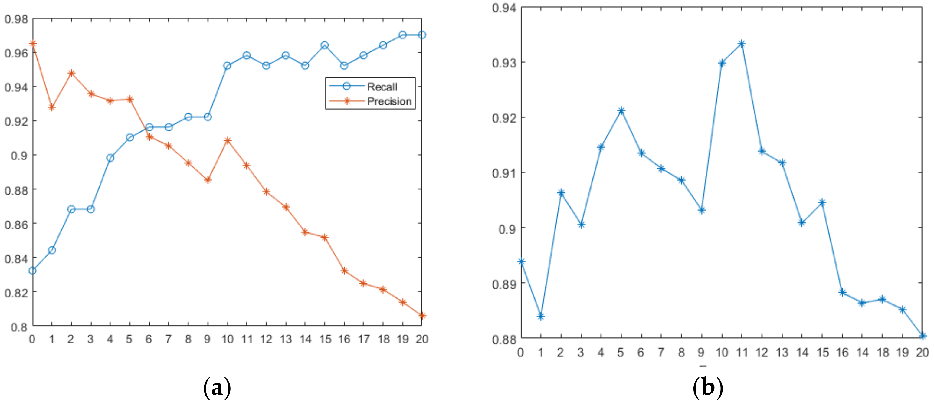
Figure 7 shows the average recall and precision calculated according to the different relative angle offset angles. As Figure 7 shows, as the relative offset of the angle increases, the value of recall increases, but the value of precision decreases. When the relative offset angle θ_d was equal to 11, the highest F-score value was obtained, and we could obtain a relatively satisfactory performance. Therefore, we set the threshold to 11.

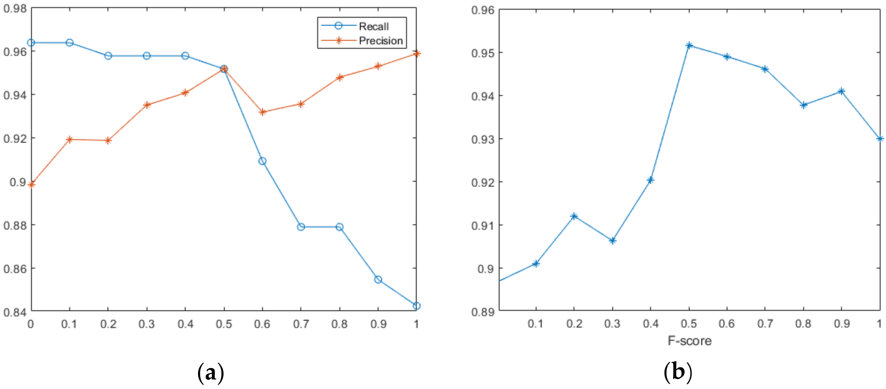
Figure 8 shows the influence of differences in d_k within [0,1] on recall and precision. d_k is a threshold of the relative length. When d_k is too small, the distance between candidate points is larger, and the incorrect point is more easily matched. When d_k is larger, although the recall is higher, the matching accuracy will be much lower. When the threshold of the relative length d_k was equal to 0.5, the highest F-score value was obtained, and we could obtain a relatively satisfactory performance. Thus, we set d_k to approximately 0.5.

According to Figure 7 and Figure 8, in the case of blurred sea ice image features with intensity differences, in order to ensure the best balance of accuracy and efficiency of the outlier strategy, we set the threshold of d_k to 0.5 and the angle threshold to 11.

4.4. Ablation Experiments

We used a global feature image patch (G), local feature image patch (L), and image patch with fusion of local and global features (GL) as input to test the experimental datasets, and the test results are shown in

Table 3. Evaluation indicators for different input patch pairs on datasets.

	Precision	Recall	F-Score
G	73.24%	72.51%	72.86%
L	89.26%	81.85%	85.33%
GL	94.33%	93.05%	93.89%

. We used three evaluation metrics commonly used in image registration, which are precision, recall, and F-score. As can be seen from Table 3, the value of the image patch with fusion of local and global features as input was the highest. The feature fused with local features and global features can contain local textural features, as well as global structural features, which can better distinguish the differences between the sea surface targets with repetitive textural features. Finally we chose to use image patches of global and local features as input.

4.5. Benchmark Comparisons on the Same Polarization Mode

By experimenting with the data in Table 2 (No.1–No.6), we used a visual comparison and three indicators to evaluate our method’s performance qualitatively. The purpose of the experiment was to compare our network algorithm with other methods. In order to make the comparison experiment fairer and more objective, our removal outlier algorithm was applied in all comparison algorithms.

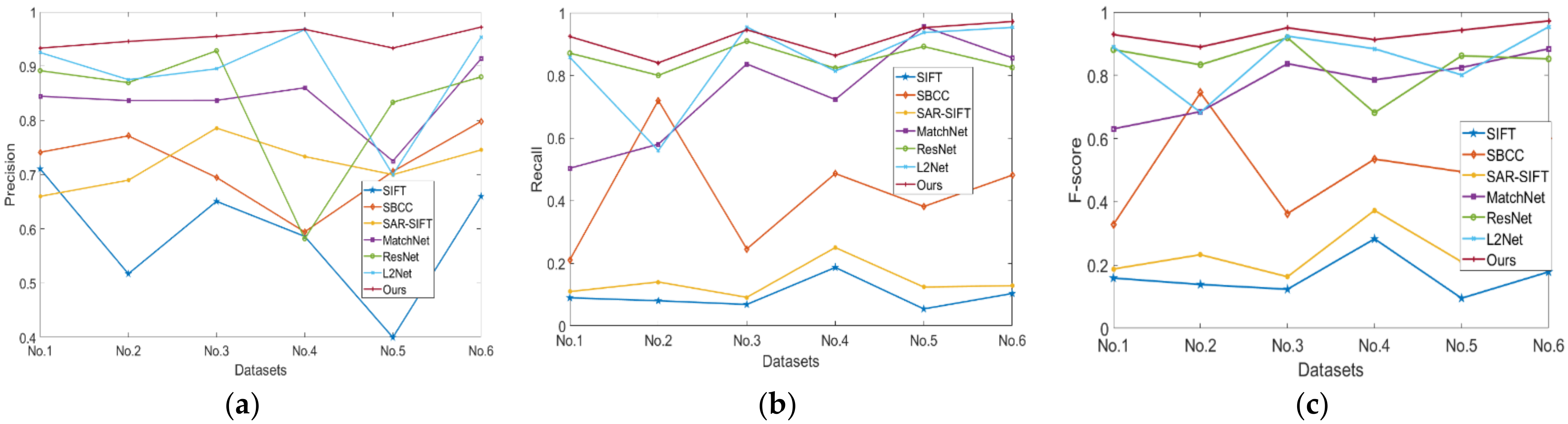
Figure 9 presents a comparison of matching precision and recall for six SAR image pairs. It is again verified by the images that the machine learning method performed better than the traditional manual descriptor matching. The average precision of our method was 95.5%. Compared with the other four deep learning algorithms (MatchNet, ResNet, L2Net), our method was better by 6.87%, 4.43%, and 3.46%, respectively. We also show the recall of all algorithms. Although the effect of individual data was similarly to the other algorithms, our algorithm could maintain a high recall rate. Our method achieved 80.3%, 48.2%, 75.5%, 4.41%, 3.46% and 2.4% improvements in the average recall compared with SIFT, SBCC, SAR-SIFT, MatchNet, ResNet, and L2Net, respectively. Therefore, our method had a stronger robustness in feature matching of heterogeneous sea ice SAR images with intensity differences. The F-score curves indicate that the F-score of our method was best. Thus, in the same polarization mode, our method achieved the best trade-off between accuracy and efficiency, while guaranteeing a sufficient number of matching points.

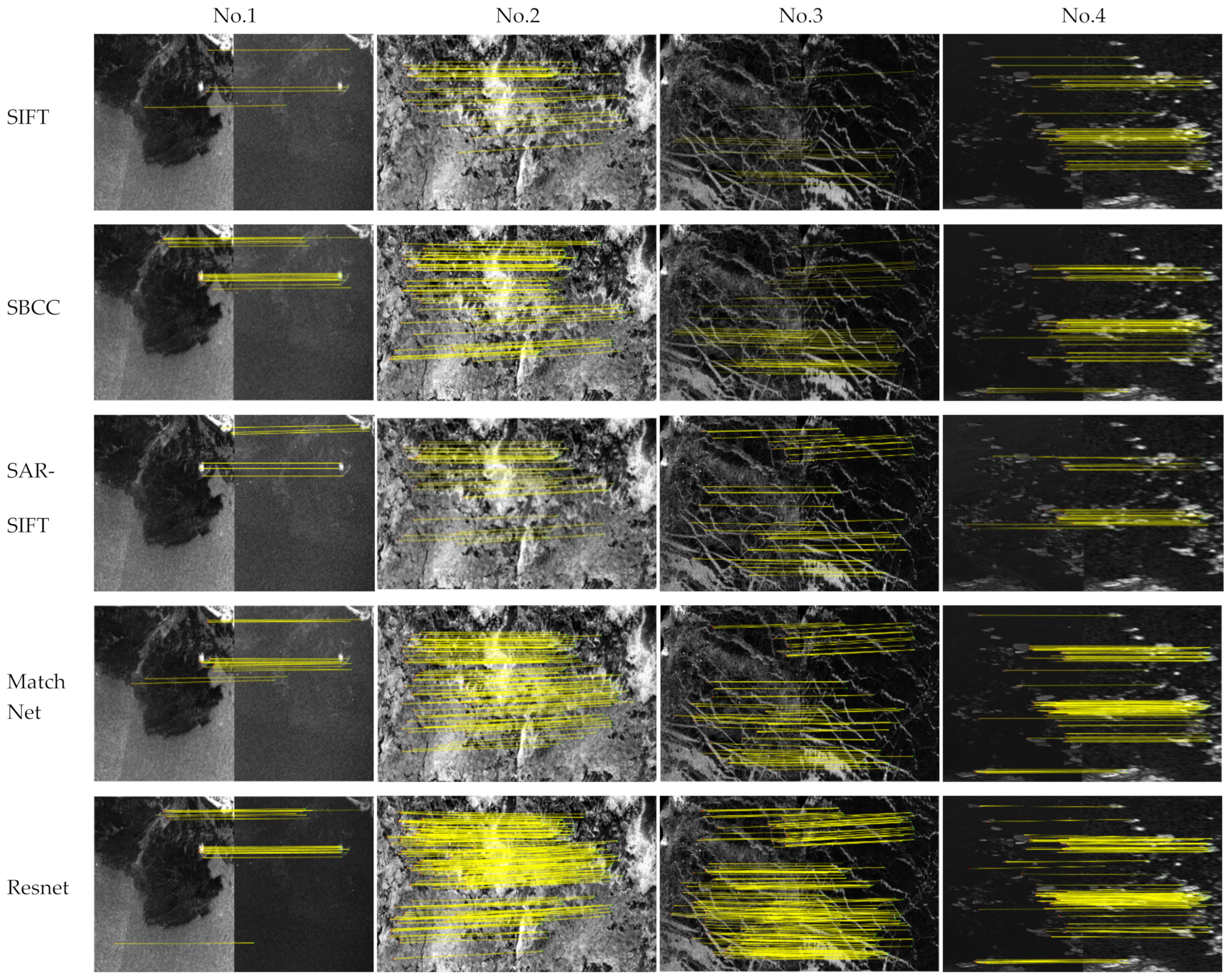
Figure 10 presents the image matching results for the image pairs (No.1, No.2, No.3, and No.4). The image matching results show that the common algorithms (SIFT, SBCC, SAR-SIFT) obtained the least matching points, and the patch matching network could obtain more matching points. Sea ice in SAR images is affected by the interaction between ocean currents and sea ice. At the same time, different satellites have different shooting times, resulting in different lighting conditions and satellite shooting angles. The final result is that the sea ice has intensity differences, and the local non-rigid deformation of sea ice eventually leads to blurred sea ice features. Therefore, it is difficult to obtain a good feature matching performance using common manual feature descriptors. In addition, the learning-based method can establish a matching vector set according to the characteristics of sea ice. The dependency between the image pair can be obtained by deep learning of the intensity difference between two existent intensities; thus, obtaining more matches. The sea ice in the Bohai Sea region is mostly thin ice, which is influenced by ocean currents, especially through the of deformation and extrusion of thin ice far from the coastline. Therefore, the overall number of matching points is small. The sea ice located in the north and south poles is mostly perennial thick ice. Thick sea ice characteristics are more stable, so the number of matches is higher.

Table 4. The Number of Point Matches.

	No.1	No.2	No.3	No.4	No.5	No.6
SIFT	4	22	15	41	27	33
SBCC	25	63	54	107	120	112
SAR-SIFT	6	33	45	63	33	39
MatchNet	29	152	184	159	301	274
ResNet	40	181	200	255	281	295
L2Net	28	179	210	259	295	305
Our method	42	190	208	279	303	324

presents the number of image matching pairs of all results on the six datasets. For the sea ice drift application, not only should the accuracy of matching be maintained, but the number of matching points should be increased. It can be seen from Table 4 that the SIFT algorithm has the least number of matching points, and the number of matching points is the most except for the third set of data. Through Table 4 we can also see that the machine learning algorithms could find more correct matching points than the common manual descriptors. The machine learning method could establish the dependency of image patch pairs with different strengths through learning. The number of point matching results of L2Net was next best to that of our method, but the precision of our method was better than that of L2Net. Thus, in the same polarization mode, our method achieved the best trade-off between accuracy and efficiency, while guaranteeing a sufficient number of matching points.

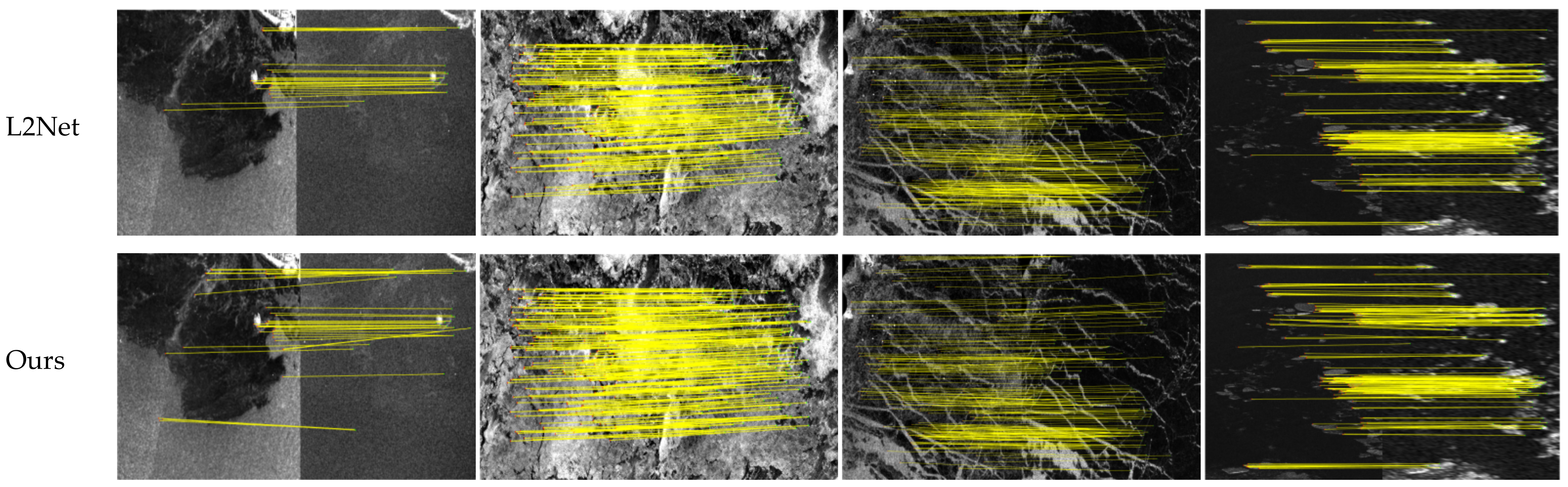
As can be seen in Figure 9 and Figure 10 and Table 4, the classical algorithms SIFT, SBCC, and SAR-SIFT correctly matched the least number of points and also had the lowest precision and recall. The classical algorithms only use intensity information, which causes numerous error matches when the image has numerous repeated features. Compared with classical feature matching algorithms, deep learning networks can learn the feature correspondence between heterogeneous SAR images with intensity differences, increasing the number of matching points, as well as improving the matching accuracy. However, several of the common deep learning algorithms do not use contextual information, which results in an incorrect match when there are numerous duplicate features. Although L2Net uses contextual relationships, the use of control point-centered small image block upsampling as input, and the use of a small image patch to extract texture features, results in poor discrimination of the presence of repetitive textural features. Moreover, our algorithm downsamples 64 × 64 image patches to 32 × 32 as input, which can obtain more contextual information and improve the feature variability between image blocks, helping to improve the accuracy of feature matching.

4.6. Benchmark Comparisons on Different Polarization Mode

The proposed method and the three other algorithms were applied to the four datasets in Table 2 (No.7–No.10) with different polarization modes, including SIFT, SBCC, SAR-SIFT, MatchNet, ResNet, L2Net; all of which achieved the removal of mismatching points.

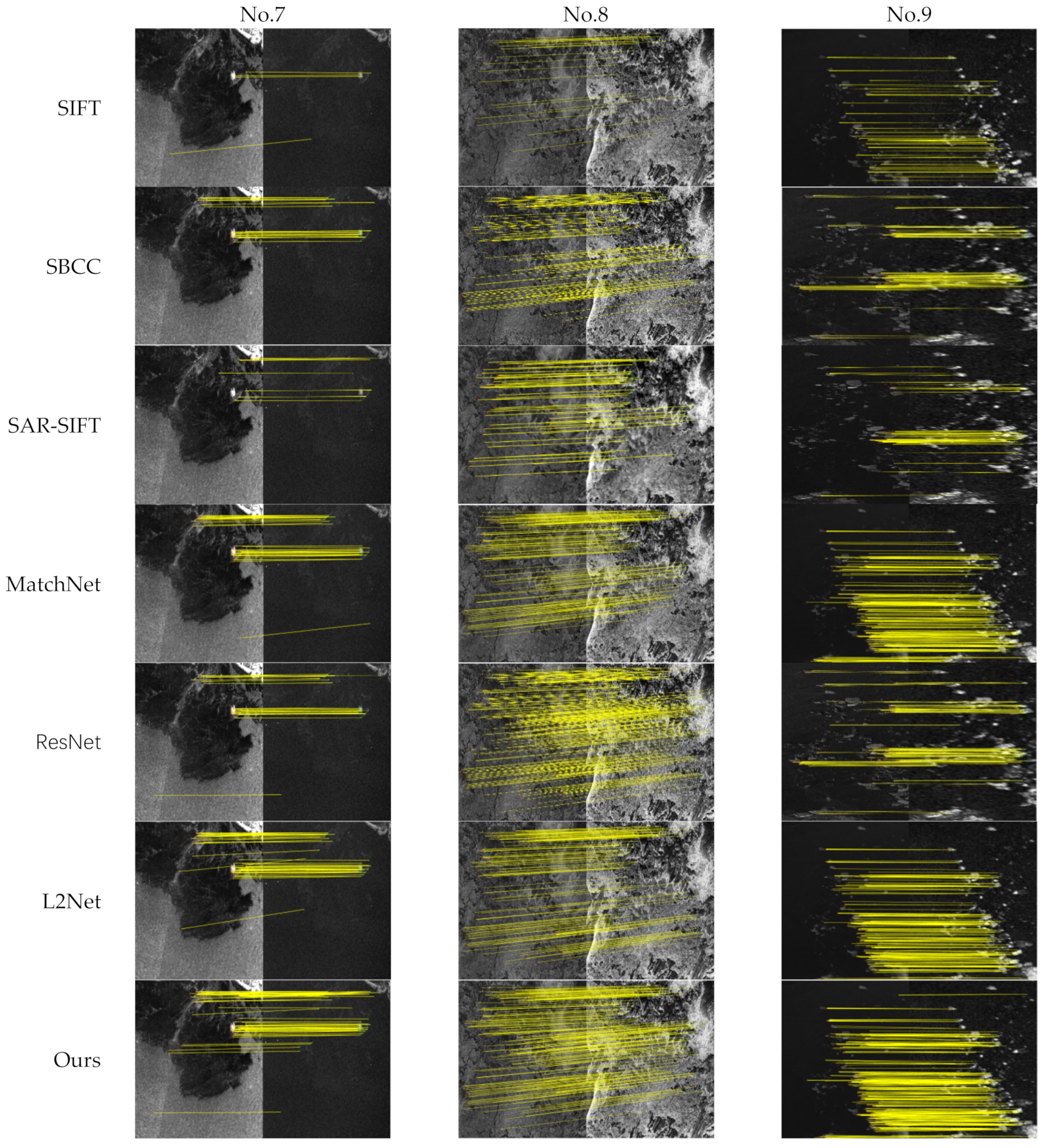
Figure 11 presents the point matching results with the three datasets (No.7–No.9). As can be seen in Figure 11, our algorithm could also obtain better matching results on SAR images with different polarization methods, compared with the other algorithms. The results of our algorithm were better than those of the other algorithms, because our algorithm uses four image patches as input and can obtain a good correlation between image patches.

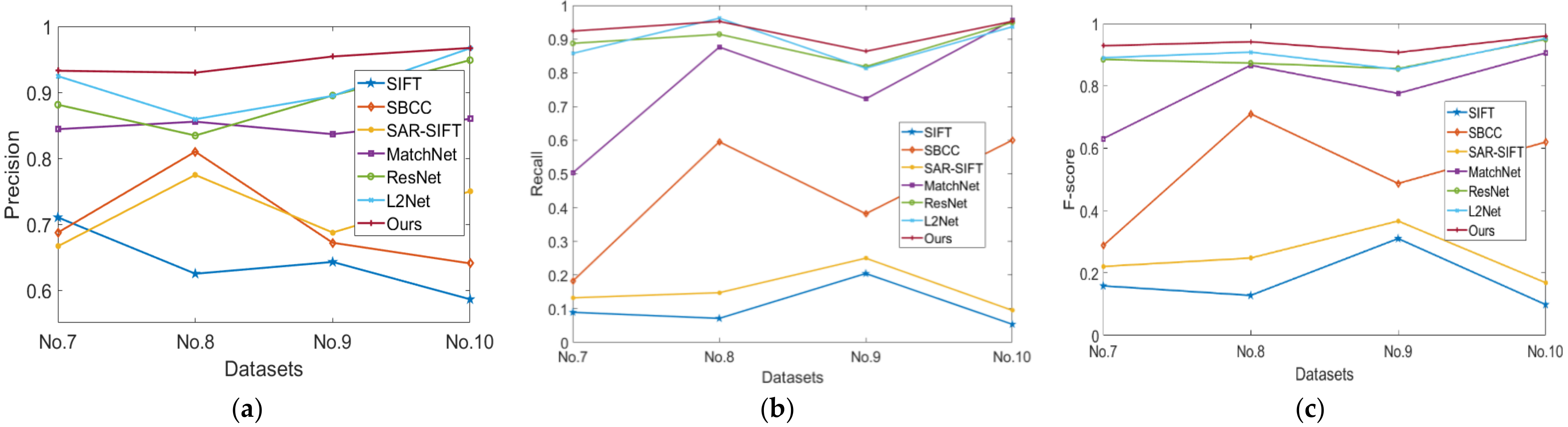
Figure 12 presents the comparison curves of the average recall and accuracy of SIFT, SBCC, SAR-SIFT, MatchNet, ResNet, L2Net, and the proposed method. Compared with SIFT, SBCC, SAR-SIFT, MatchNet, ResNet, and L2Net, our method’s average precision increased by 32.3%, 24.4%, 26.7%, 9.86%, 5.6%, and 4.62%, respectively. The average recall rate was increased by 78.6%, 48.7%, 69.8%, 10.9%, 2.99%, and 2.14%, respectively. The results show that our method not only achieved the highest accuracy for the test datasets of different polarization modes, but also almost always achieved the highest recall rate. The F-score curves indicate that the F-score of our method was also the best. Thus, in the different polarization modes, our method also achieved the best trade-off between accuracy and efficiency, while guaranteeing a sufficient number of matching points.

Table 5. The Number of Point Matches.

	No.7	No.8	No.9	No.10
SIFT	4	27	36	19
SBCC	20	109	50	63
SAR-SIFT	5	44	49	31
MatchNet	37	124	159	241
ResNet	62	147	160	226
L2Net	51	198	214	239
Our method	76	206	229	248

presents the results of the seven different matching algorithms, in terms of the number of matching points for the four sets of experimental data with different polarization algorithms. Our algorithm could also obtain a high number of matching points with datasets with different polarization modes. From Table 5, the number of matches obtained by the traditional feature descriptors was significantly smaller than that of the other five deep learning algorithms. In the fourth group of data with different polarization algorithms, the five deep learning algorithms obtained an approximate number of matches, but in the four groups of images with different polarization methods, our algorithm obtained significantly higher numbers than the other deep learning algorithms. Thus, it was sufficient to provide reliable feature matching points. It can be seen that the proposed algorithm outperformed SIFT, SBCC, SAR-SIFT, MatchNet, ResNet and L2Net.

As can be seen in Figure 11 and Figure 12 and Table 5, the classical intensity-based and feature-based algorithms correctly matched the fewest points, with the lowest accuracy at the same time, when the intensity difference between images with different polarization methods in non-homogenous data was large, while the deep learning algorithms were able to obtain a higher number of matching points. The precision of deep learning algorithms such as MatchNet and ResNet, which have only two image patches as input and lack contextual relationships, was lower than L2Net and our algorithm, because of the large number of repetitive textural features in the image patches, resulting in a lower precision and recall. L2Net uses four-image patches as input, which contains certain contextual relationships and improves on the matching results. However, L2Net’s four image patches as input contains certain contextual relationships, using 16 and 32 window size image patches as the input; and for the ocean SAR images when the resolution was not high, the effective information of the obtained images was not sufficient, so the improvement of the control point feature description was limited. Compared with L2Net, this paper used a 64 × 64 image block and downsampled it to 32 × 32 as input, to obtain more contextual information around the control points; while adding the feature descriptions obtained from the 32 × 32 image patches in the original image could more effectively distinguish the differences with the presence of repetitive textural features.

5. Disscusion

The results are encouraging and show that our method can increase the performance in heterogeneous sea ice SAR image feature matching. We calculated the average recall, precision, and the standard deviation of experimental data with the same polarization method and different polarization mode, as shown in

Table 6. Average recall and precision of the same polarization mode and different polarization modes.

	The Same Polarization Mode	Different Polarization Modes
Recall	0.929024	0.960522
Precision	0.912439	0.958255
Standard deviations of precision	0.23294	0.22879

. The standard deviation of precision with the same polarization was higher than that of the data with different polarization. We found that the precision of the data with different polarization methods was 4.58% higher, and the recall was 3.12% higher, than that of the data with the same polarization methods for the same parameters. This is because the cross polarization mode HV was used in different polarization mode. HV channel is more suitable for sea ice drift studies than the HH channel in situations where the HV signal is higher than the noise floor.

The results of experiments on 10 experimental datasets show that our proposed algorithm for sea ice feature matching not only improved the recall rate but also the matching accuracy compared to SIFT, SBCC, SAR-SIFT MatchNet, ResNet, and L2Net. Our algorithm could obtain the maximum number of matching points with guaranteed correctness, and also provided many reliable sea ice matching points for the sea ice drift detection process. Therefore, our method had a good effect on the matching of heterogeneous sea ice features with different strengths. It not only improved the matching accuracy, but also slightly improved the matching recall rate.

6. Conclusions

In this paper, we proposed a novel repetitive texture image registration for SAR images with intensity differences. The network proved able to correlate features between sea surface objectives with repetitive textural features and could establish the dependency between two image patches with intensity differences through deep learning. We increased the dual input of the common Siamese network to four inputs. In the sea ice SAR image pair, two patches of different sizes, centered on the corner points, were used as input. The two additional inputs were a small image patch obtained by downsampling the large image patch. In this way, local features and more global features were fused to obtain better differentiation of object structure information and add contextual information. Contextual information improved the discrimination of repetitive textures and the accuracy of image registration. Using the characteristics of sea surface objectives, a suitable error match point removal strategy for SAR images was proposed. In this paper, with sea ice as the object of study, the experimental results of the measured heterogeneous SAR images showed that the algorithm could effectively overcome nonlinear intensity changes and obtain better image matching results. The results indicated that, compared with the other six commonly used algorithms, our algorithm was more accurate and robust.

The common sea surface objectives in SAR image registration are sea ice, oil spills, and enteromorpha, and they all have a large amount of repetitive texture. The data used in this paper are historical data, with a relatively long time interval. If data with a short enough time interval were used, the application scenario of the algorithm in this paper could cover the field of repetitive textures, such as sea ice, oil spills, and enteromorpha.