Article

Convective Entrainment Rate over the Tibetan Plateau and Its Adjacent Regions in the Boreal Summer Using SNPP-VIIRS

1
Collaborative Innovation Center on Forecast and Evaluation of Meteorological Disasters, Key Laboratory for Aerosol-Cloud-Precipitation of China Meteorological Administration, Nanjing University of Information Science & Technology, Nanjing 210044, China
2
Center of Weather Modification of Shaanxi Province, Xi’an 710016, China
3
Department of Geological and Atmospheric Sciences, Iowa State University, Ames, IA 50011, USA
4
Nanjing Joint Institute for Atmospheric Sciences, Nanjing 210019, China
5
College of Aviation Meteorology, Civil Aviation Flight University of China, Guanghan 618307, China
6
Department of Geography, Faculty of Social Sciences, Hong Kong Baptist University, Hong Kong 999077, China
*
Author to whom correspondence should be addressed.
Remote Sens. 2022, 14(9), 2073; https://doi.org/10.3390/rs14092073
Submission received: 25 March 2022 / Revised: 23 April 2022 / Accepted: 24 April 2022 / Published: 26 April 2022
(This article belongs to the Special Issue Remote Sensing of Clouds and Precipitation at Multiple Scales II)

Abstract

:
The entrainment rate (λ) is difficult to estimate, and its uncertainties cause a significant error in convection parameterization and precipitation simulation, especially over the Tibetan Plateau, where observations are scarce. The λ over the Tibetan Plateau, and its adjacent regions, is estimated for the first time using five-year satellite data and a reanalysis dataset. The λ and cloud base environmental relative humidity (RH) decrease with an increase in terrain height. Quantitatively, the correlation between λ and RH changes from positive at low terrain heights to negative at high terrain heights, and the underlying mechanisms are here interpreted. When the terrain height is below 1 km, large RH decreases the difference in moist static energy (MSE) between the clouds and the environment and increases λ. When the terrain height is above 1 km, the correlation between λ and RH is related to the difference between MSE turning point and cloud base, because of decreases in specific humidity near the surface with increasing terrain height. These results enhance the theoretical understanding of the factors affecting λ and pave the way for improving the parameterization of λ.

Graphical Abstract

1. Introduction

With a mean elevation of 4 km above sea level, the Tibetan Plateau (TP) is known as the third pole of the world and plays a crucial role in regional atmospheric circulation and global climate (e.g., [1,2,3,4,5]). As the ‘atmospheric heat pump’ [6] and ‘atmospheric water tower’ [7] in boreal summer, the TP provides favorable conditions for local convection. Meanwhile, downstream clouds and precipitation are significantly affected by the convection of TP (e.g., [8,9,10]).
Clouds have significant effects on the atmospheric energy budget [11,12,13,14,15], while cloud processes over the TP are quite unique to those over other regions of China (e.g., [16,17]). The frequency of cloudy days is especially high over the TP [18,19], and cloud frequency is 73.6% over the TP in boreal summer [19]. The clouds over the TP exhibit a low cloud base height [20] and small cloud depth [21,22]; the clouds with a cloud depth less than 2 km have the highest frequency [21]. Affected by the high elevation and unique cloud properties over the TP, clouds and precipitation are difficult to simulate accurately. The reasons for the uncertainties vary: including the uncertainty of forcing data, low model resolution, and the uncertainty of parameterization (e.g., [23,24,25,26]). For example, Luo et al. [24] found that the uncertainty of entrainment rate (λ) in the cumulus convection scheme is an important reason for the simulation error of convective precipitation over the TP.
The λ, which describes the rate of environmental air mixed into cloud, is a crucial parameter for convection parameterization in simulations [27,28,29,30,31]. Convection parameterization is a vital factor in weather and climate models [32,33,34], and uncertainties in λ can lead to large deviations in weather and climate simulations (e.g., [35,36,37]). Previous studies have related λ to cloud dynamical and thermodynamic properties [38,39,40] and environmental conditions [41,42,43,44]. Buoyancy and vertical velocity are found to be negatively correlated with λ [45,46,47]. Aerosols have a significant effect on entrainment through the evaporation–entrainment feedback mechanism [41,48,49,50]. The relationship between λ and relative humidity is unresolved; the two quantities have been identified as positively [51,52,53,54,55,56,57], negatively [58,59,60,61], or weakly correlated [57,61]. Based on the above factors and others [62,63,64] (e.g., height [65,66]), many λ parameterizations have been developed [43,45,67,68,69,70]. However, as demonstrated by de Rooy et al. [71], there is no sign of convergence towards certain parameterizations. It is also challenging to determine which factors are most important for parameterizing λ. Hence, further studies are necessary to examine the factors affecting λ and to develop parameterizations of λ.
Traditionally, the results of high-resolution simulations (e.g., [68]) and aircraft observations (e.g., [43,72]) have been used to estimate λ. However, the harsh environment of the TP restricts the necessary observations to improve the model’s initial forcing [73], and aircraft observations are rare [74]. In addition, compared with these case studies, an λ, based on long-term averaged data, is required to provide more information with larger spatial and temporal scales. Hence, satellite data, which covers a long period, are more accessible for estimating λ over the entire TP. Luo et al. [75] were the first to use satellite data to estimate λ, using an entrainment plume model, and this method has been applied in many studies [57,64]. Wang and Zhang [36] also estimated λ from satellite data to evaluate the accuracy of λ in the community atmosphere model.
To the best of our knowledge, many studies about the development of convection over the TP have been carried out [20,76], but studies about convection over the TP in the perspective of entrainment are lacking. Entrainment plays an important role in convection through cloud interaction with the environment, but there have been no studies on λ over the TP, not even case studies. Based on five-year data from the Visible Infrared Imaging Radiometer Suite (VIIRS) onboard the Suomi National Polar-orbiting Partnership (SNPP) satellite [77], this study is the first to estimate λ over the entire TP and its adjacent regions. The results will enhance the understanding of λ and help to improve the accuracy of convective precipitation simulation over the TP. The remainder of this paper is organized as follows. Section 2 describes the data and methodology used in this study. Section 3 presents spatial distribution and factors affecting the λ. Section 4 provides a summary of the study.

2. Method

Based on the Automated Mapping of Convective Clouds system, described by Yue et al. [78], and the SNPP-VIIRS satellite data, Yue et al. [79] retrieved the characteristics of convective clouds at cloud top and base over the TP, and its adjacent regions, at approximately 07:00 UTC (from 05:00 to 09:00 UTC, in the local afternoon) from June to August 2013 to 2017. The method to obtain the cloud base and cloud top temperature is described by Yue et al. [79] in detail. The cloud base temperature is calculated based on the warmest cloudy pixels of VIIRS [78,80], and the cloud base environmental temperature is interpolated, based on the environmental profile from the reanalysis dataset and the cloud base height. The cloud top temperature is calculated based on the coldest cloudy pixels of VIIRS [78,79], and the cloud top environmental temperature is assumed to be equal to the cloud top temperature to obtain the cloud top height. The way to retrieve other variables can be seen in Yue et al. [78]. The convective cloud cases are averaged to 0.33° × 0.33° convective cloud product grids to obtain the averaged convective characteristics over the TP, and its adjacent regions, in boreal summer. According to Yue et al. [78], retrieved convective clouds are driven by surface thermal effects in the afternoon and have a flat cloud base at the lifting condensation level.
The ERA-Interim reanalysis dataset [81] performs better than other reanalysis datasets over the TP [82,83], and the fifth-generation European Centre for Medium-Range Weather Forecasts reanalysis (ERA5) [84] dataset, which is the successor of the ERA-Interim, is closer to the rawinsondes over the TP [73]. Differing from the NCEP final operational global analysis data [85] used by Yue et al. [79], the hourly ERA5 is used to provide the vertical structure of meteorological elements. ERA5, with a resolution of 0.25° × 0.25°, is interpolated to the correct locations to obtain environmental profiles of convective cloud cases. The environmental profiles are averaged to 0.33° × 0.33° grids of the convective cloud product.
To make the results more representative, grids in the convective cloud product with fewer than 10 convective cloud cases are eliminated. The cloud base temperature deviation is defined as the deviation between cloud base temperature inside and outside of the clouds. The mean value and standard deviation of cloud base temperature deviation in convective cloud grids were calculated. The grids were eliminated if their cloud base temperature deviations were beyond the range from the mean minus standard deviation to the mean plus standard deviation. The maximum value of either environmental moist static energy (MSE) under the cloud base or cloud base in-cloud MSE was chosen to be the cloud base in-cloud MSE, because the level of the maximum value of MSE is considered to be the convection starting level [86,87]. Grids with a cloud base in-cloud MSE less than the cloud top in-cloud MSE were eliminated, because, according to Wang and Zhang [36], the in-cloud MSE increases with height when detrainment dominates over entrainment and will be unreasonably higher than the cloud base in-cloud MSE if there is too much detrainment. After the elimination, there were a total of 2214 grids, and Figure 1 presents the locations and case numbers of the convective cloud product grids. The high number of cases over southeastern TP indicates a high frequency of convection activities over the area [19,76].
Based on the approaches of Zhang et al. [27], λ is considered to be the difference in the conserved MSE between the air inside and outside the cloud:
λ = d h c / d z h c h e ,
where hc and z are the in-cloud MSE and height (hereafter, the height denotes the height above sea level, if not specified) at the cloud base and cloud top from the convective cloud product, respectively, and he is the mean environmental MSE from ERA5. It is important to note that λ calculated in this research denotes the mean entrainment in the layer dz.
Considering that the melting level is near the surface, and ice particles contribute significantly to clouds over the TP [21], the freezing and melting process must be taken into account [88]. Hence, following Muller and Held [88], the MSE including ice-phase processes is given:
h = c p T + g z + L v q v L f q i
where cp is the isobaric specific heat of dry air, T is the temperature, g is the acceleration due to gravity, Lv is the latent heat of vaporization, qv is the specific humidity, Lf is the latent heat of fusion, and qi is the specific cloud ice content, including precipitating and non-precipitating ice phases. Since there are no specific cloud ice contents in the environment, the specific cloud ice contents in ERA5 are divided by the fraction of cloud cover and used for the convective cloud product. To account for the contribution of latent heat of freezing, λ without considering latent heat of freezing is also calculated; the difference between λ with and without considering latent heat of freezing is from –0.02 to 0.52 km−1, with a median of 0.003 km−1, a mean of 0.03 km−1, and a standard deviation of 0.07 km−1.

3. Result

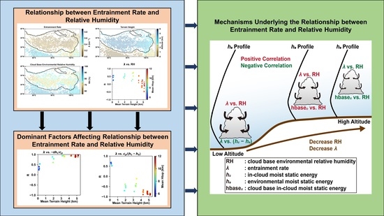
3.1. Relationship between Entrainment Rate and Relative Humidity

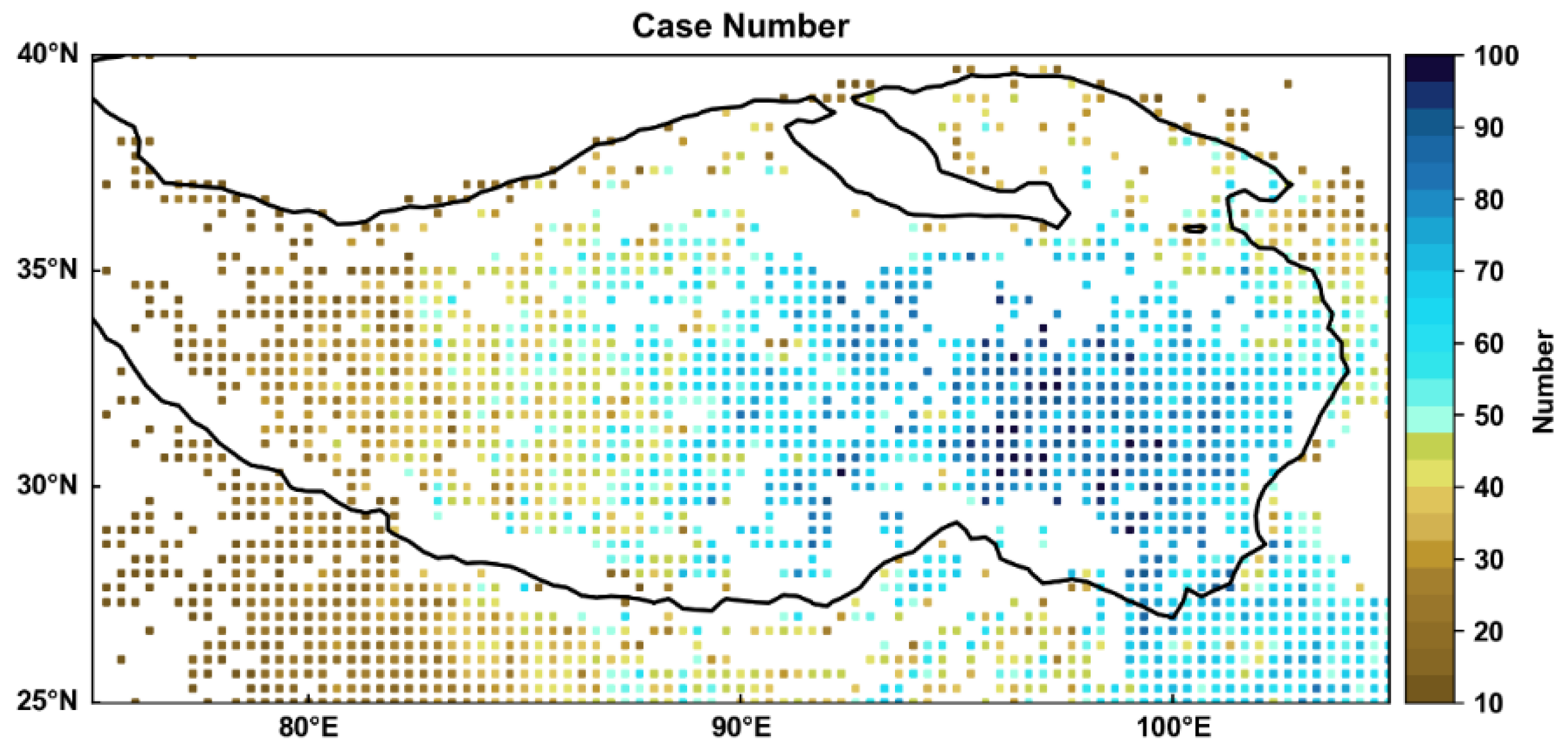
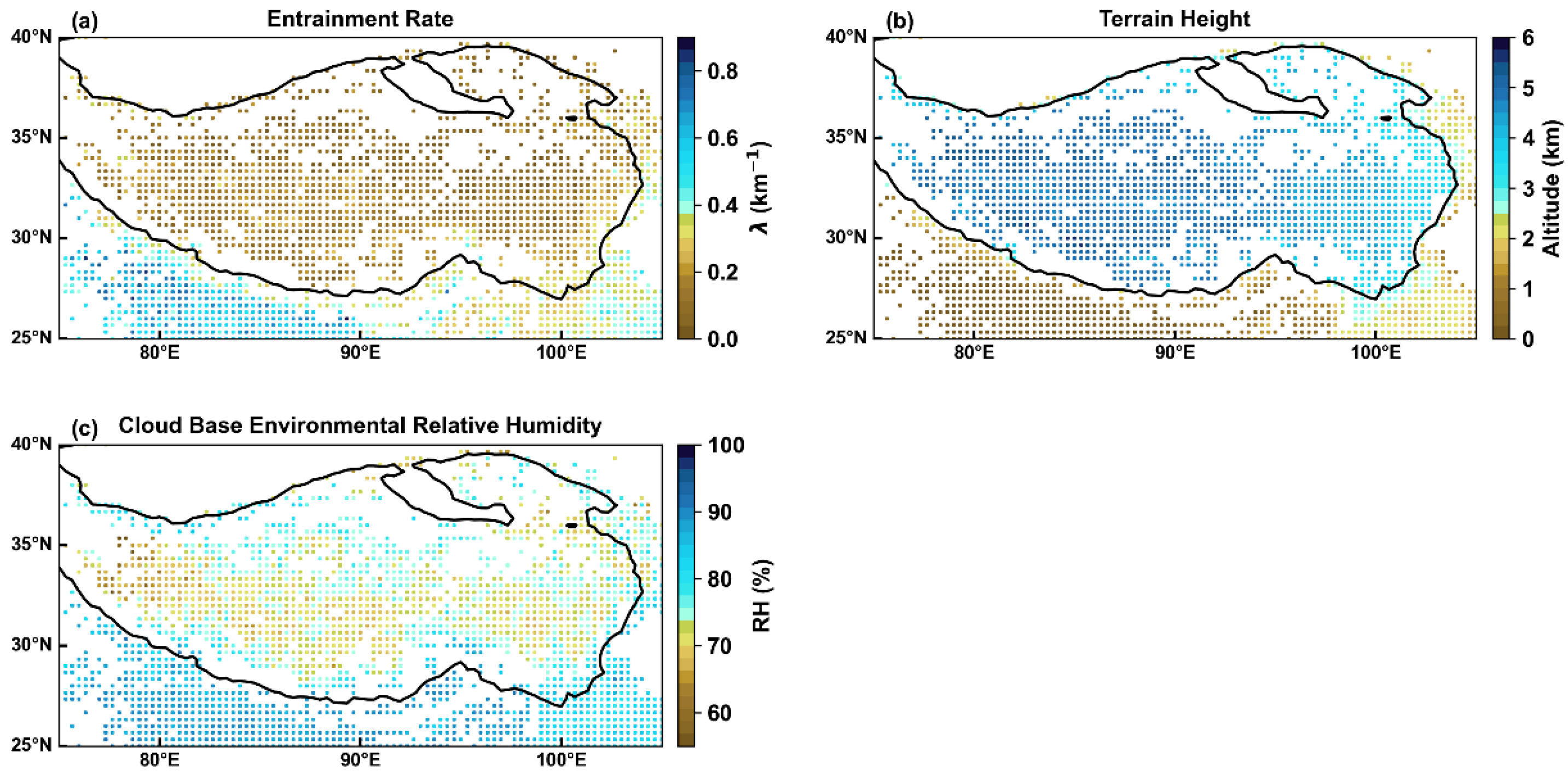
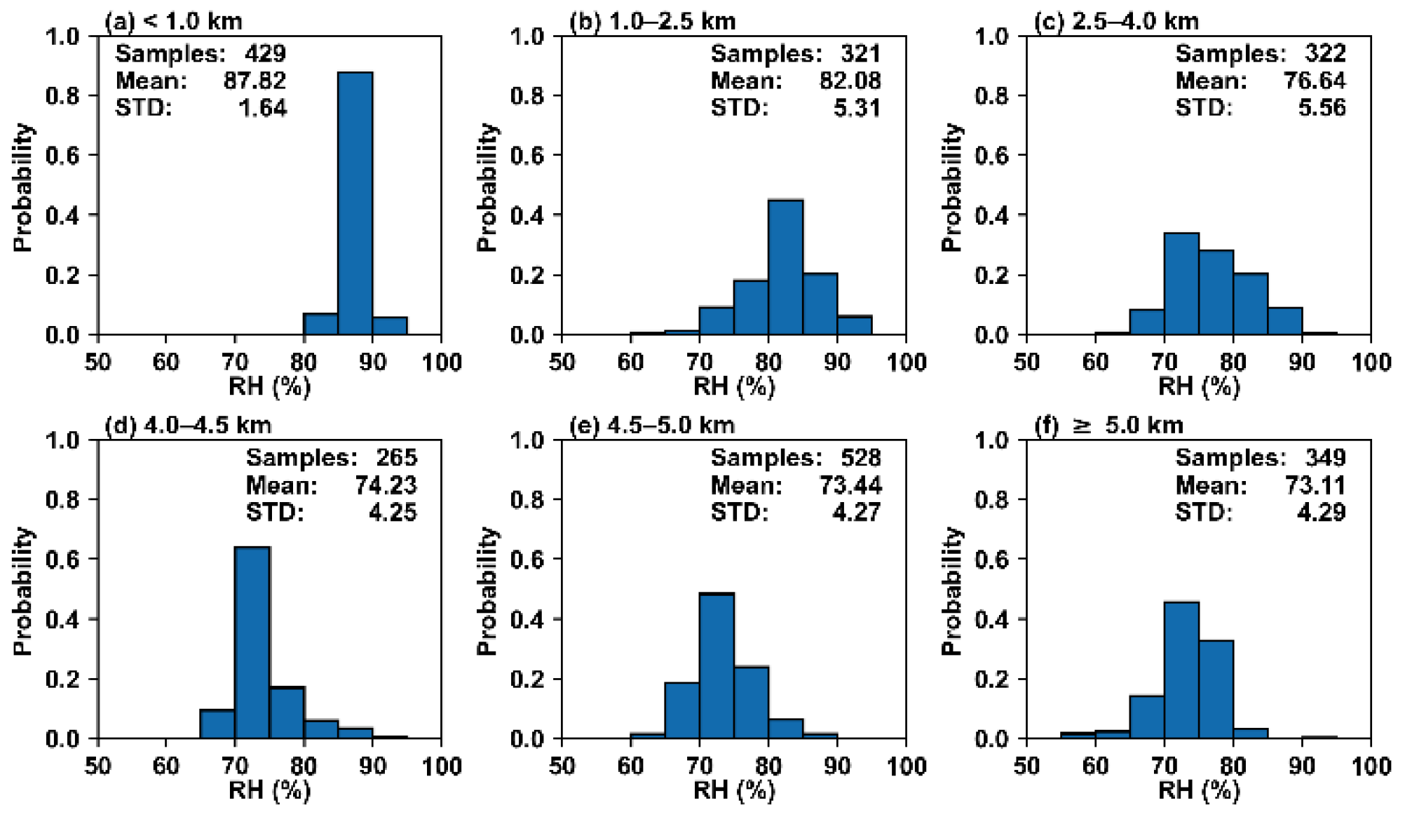
3.1.1. Effects of Terrain Height on Entrainment Rate and Relative Humidity

Based on the SNPP-VIIRS-based convective cloud product, Figure 2 presents distribution of λ, terrain height, and cloud base environmental relative humidity (RH) over the studied region in boreal summer from 2013 to 2017. The values of λ are less than 0.90 km−1. Generally, the largest values of λ and RH are both predominantly in the southwest of the studied region, with a terrain height below 3 km, and the smallest values of λ and RH are primarily in the region with a terrain height above 3 km.
To further analyze the relationship between λ and RH, the grids are divided into 6 groups according to terrain height, and the sample numbers within each terrain height groups are similar: <1.0 km, 1.0–2.5 km, 2.5–4.0 km, 4.0–4.5 km, 4.5–5.0 km, and >5.0 km. The probability density distribution (PDF) of λ for different terrain height ranges is provided in Figure 3. The region with a terrain height below 1 km has the largest mean λ of 0.55 km−1 and the widest distribution range of λ, which ranges from 0.20 to 0.90 km−1. As the terrain height increases, the values of λ decrease, and the distribution range of λ also becomes narrower. The region with a terrain height above 5 km has the smallest mean λ of 0.12 km−1 and the narrowest distribution, the maximum value of which is less than 0.40 km−1. The PDF of the RH for different terrain height ranges is displayed in Figure 4. The RH ranges from 55% to 95%. The region with a terrain height below 1 km has the narrowest PDF of RH, with the largest mean RH of 87.8%. As terrain height increases, the values of RH decrease. The region with a terrain height above 5 km has the smallest mean RH of 73.1%. Therefore, λ and RH both exhibit a decreasing trend with an increase in terrain height.

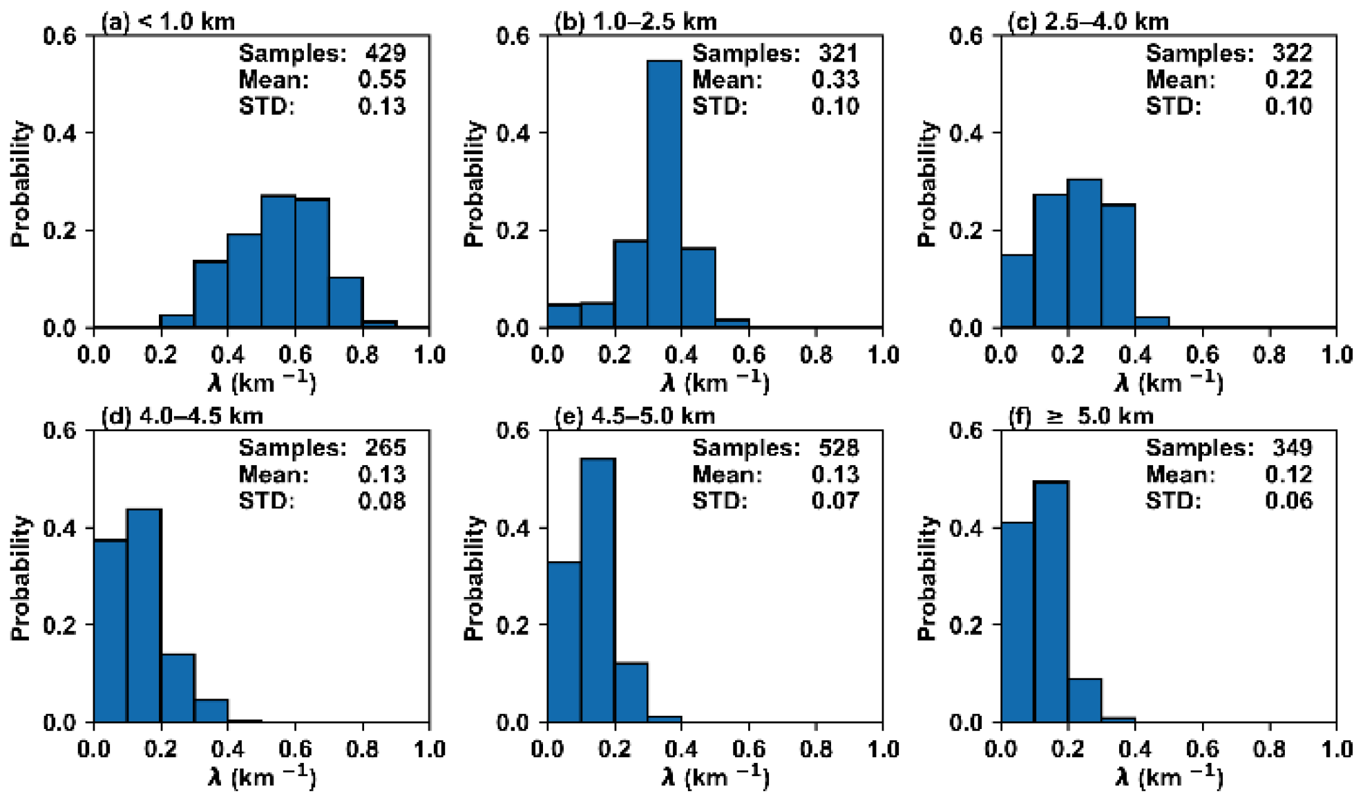
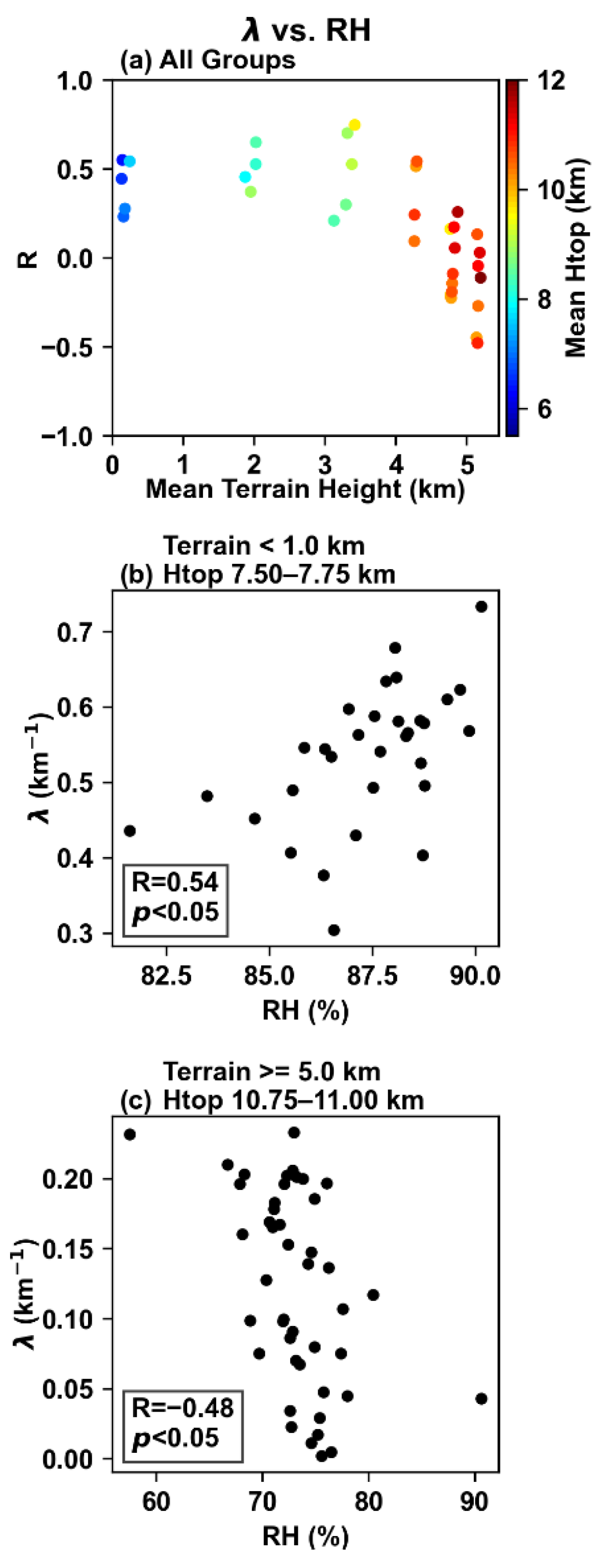
3.1.2. Quantitative Relationships between Entrainment Rate and Relative Humidity in Different Terrain Height Ranges

The qualitative analysis in Section 3.1.1 indicates a positive relationship between λ and RH. A quantitative analysis is further conducted to verify the reliability of the conclusion. The grids are still divided into six groups, based on terrain height, as described in Section 3.1.1. To minimize the impacts of meteorological conditions and ensure the clouds have relatively uniform characteristics, the cloud samples are further divided according to cloud top height within each terrain height range, following Liu et al. [89]. The cloud samples are grouped every 0.25 km for cloud top height from less than 5.50 km to greater than 12.00 km. Only the groups with more than 30 samples are analyzed to ensure that the sample size is sufficiently large.
The correlation coefficients of λ and RH for different cloud groups are illustrated in Figure 5a. Two representative groups of the relationship between λ and RH are also shown in Figure 5b,c. The relationships are positive in most groups and generally change from positive to negative when terrain height increases. Currently, there is no consensus on the relationship between λ and relative humidity. This relationship can be positive [51,52,53,54,55,56,57] or negative [58,59,60,61]. Recently, Xu et al. [68] even found a non-monotonic relationship: positive at low height and negative at high height, also using the MSE as the conserved property to estimate λ with cloud-resolving model simulations. Stanfield et al. [57] found a positive relationship in the Goddard Earth Observing System simulations, with no obvious relationship in the satellite results, using carbon monoxide as the conserved property to estimate λ. Eissner et al. [63] found a weak positive correlation between λ and relative humidity based on radar results, using equivalent potential temperature as the conserved property.
Previous studies have suggested that the positive correlation between λ and RH could be explained by the following mechanism: a higher RH corresponds to a smaller difference in MSE between the cloud and the environment, smaller buoyancy and vertical velocity, and higher λ [43,45]. Moreover, positive correlation between λ and RH can also be explained by the concept of buoyancy sorting, whereby more parcels are likely to be entrained into the cloud in an environment with higher RH [43,90]. Further to the above two arguments, positive correlation between λ and RH could also be explained by the following mechanism: lower RH corresponds to higher cloud base height [91], which further increases vertical velocity, since vertical velocity increases nearly linearly with cloud base height [92,93]; stronger vertical velocity further leads to smaller λ [45,46]. However, the above arguments cannot explain negative correlation between λ and RH. Furthermore, according to Equation (1), the above argument is based on the denominator, that is, the difference between in-cloud and environmental MSE determines λ; the numerator is neglected. The following analysis indicates that the denominator can only explain the positive correlation between λ and RH over the region with a terrain height below 1 km. For positive and negative correlations between λ and RH over the region with a terrain height above 1 km, the numerator is the key factor. In addition, although ERA5 shows better performance over the TP, compared to other data, the restrictions of ERA5 over the TP are still noteworthy. The inherent uncertainty in a small value of specific humidity in ERA5 [73,94] could weaken correlations between λ and RH, especially those found at terrain heights above 5 km.

3.2. Physical Mechanisms of Relative Humidity Affecting Entrainment Rate

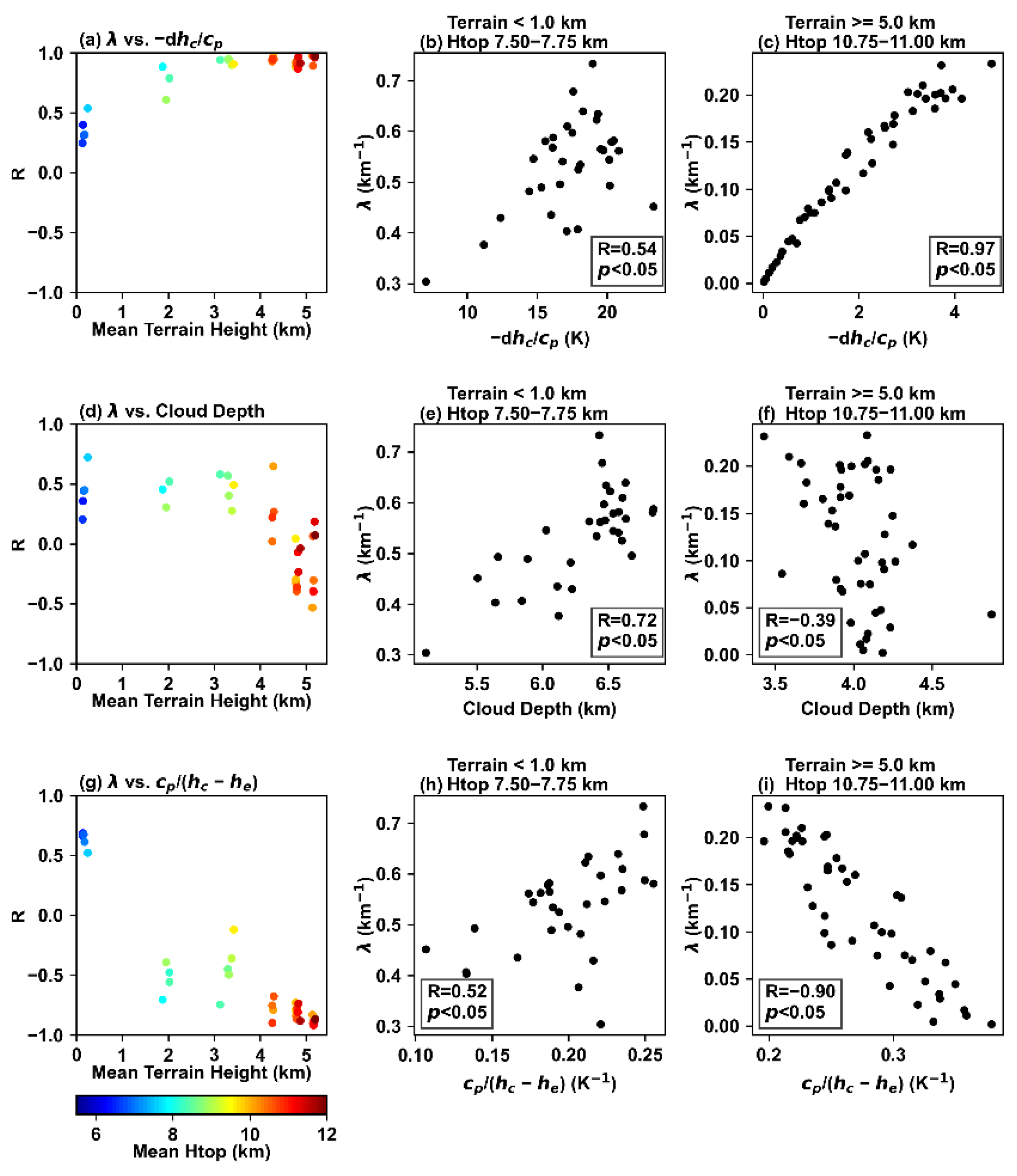
3.2.1. Dominant Factors Affecting Relationships between Entrainment Rate and Relative Humidity

To explain the relationship between λ and RH, correlation coefficients between λ and each term in Equation (1) in different cloud groups are presented in Figure 6, including the difference in in-cloud MSE between cloud base and top (−dhc), cloud depth (dz), and the reciprocal of the difference between in-cloud and environmental MSE (1/(hche)). Two representative groups of the relationship between λ and each of the above terms are also shown in Figure 6. According to Equation (1), λ is expected to be positively, negatively, and positively correlated with −dhc, dz, and 1/(hche), respectively. Figure 6 demonstrates that λ is always positively correlated with −dhc. However, the signs of λ versus dz and λ versus 1/(hche) change with terrain height.
Based on the correlation coefficients of the three relationships, Figure 6 can be divided into two groups. In Group One, having terrain height below 1 km, the correlation between λ and dz is unexpectedly positive, while a negative correlation between the two quantities was found in some previous studies [58,95]. The positive correlation between λ and 1/(hche) is stronger than that between λ and −dhc (Figure 6a,g), indicating the effects of 1/(hche) and −dhc on λ are greater than that of dz on λ. Therefore, 1/(hche) is the key factor affecting λ, which is consistent with the results of previous studies: other factors being equal, the greater the difference between in-cloud and environmental MSE the more this difference promotes an increase in vertical velocity in the cloud [96], which further decreases the time for interaction between the cloud and environment [43,45] and decreases λ. The data points having terrain height above 1 km are considered to be Group Two. From 1 to 4.5 km, the correlation between λ and −dhc is strong, and the other two correlations are not consistent with the theoretical expectations of Equation (1). Above 4.5 km, although the negative correlation between λ and dz is consistent with the theoretical expectation of Equation (1), its correlation coefficient is much smaller than that between λ and −dhc (Figure 6a,d). Therefore, in contrast with the previous conclusion that the correlation between λ and RH is primarily determined by 1/(hche), we found that −dhc dominates in Group Two. The −dhc represents the change in in-cloud MSE, but the mechanism underlying the correlation between λ and RH achieved by −dhc remains unclear. Therefore, the following analysis focuses on the mechanisms related to −dhc in Group Two.

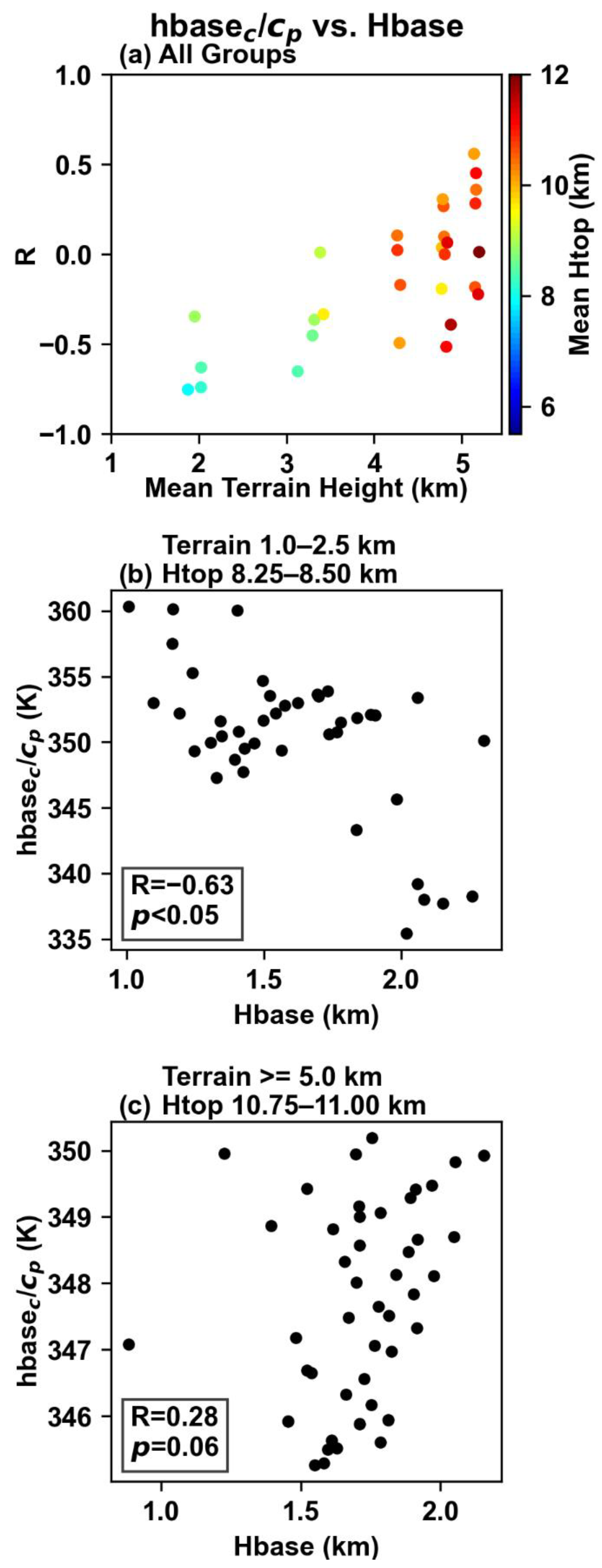
3.2.2. Critical Factor: MSE Turning Point versus Cloud Base Height

Theoretically, the greater the environmental relative humidity, the lower the cloud base height [91]; therefore, relative humidity is a direct factor affecting cloud base height and could further affect cloud base in-cloud MSE and −dhc. Figure 7a presents the correlation coefficients between cloud base in-cloud MSE and cloud base height above the surface in Group Two. Two representative groups of the relationship between cloud base in-cloud MSE and cloud base height above the surface are also shown in Figure 7b,c. When terrain height is low, cloud base in-cloud MSE is negatively correlated with cloud base height above the surface with a correlation coefficient of about −0.5. With increase in terrain height, the correlation coefficients have both positive and negative values. Hence, the relationship between cloud base in-cloud MSE and cloud base height above the surface also changes with increasing terrain height. Similar to Figure 7, but for relationships between cloud base in-cloud MSE and cloud base environmental MSE, Figure 8 further demonstrates that the quantities are positively correlated. Therefore, vertical variation in the cloud base environmental MSE reasonably represents the trend of cloud base in-cloud MSE.
Figure 9 displays the environmental MSE profiles for the different terrain height groups. Environmental MSE first decreases and then increases with increasing height in each group. The height of the environmental MSE turning point above the surface in the high terrain height ranges is smaller than that in the low terrain height ranges. To determine the reasons, the vertical profiles of the environmental dry static energy and latent heat terms of water vapor are also plotted in Figure 9, because, according to Equation (2), the MSE is composed of the above two terms; in addition, the term Lfqi is zero in the environment. Dry static energy is conserved under dry adiabatic conditions [97,98], because the rate of change of gravitational potential energy (gz) in vertical is equal to that of dry air enthalpy (cpT) in vertical under dry adiabatic conditions. However, the actual atmosphere is often not in a dry adiabatic state, and the temperature lapse rate is less than the dry adiabatic lapse rate [99]. Therefore, the rate of change of gz in vertical is larger than that of cpT in vertical, which increases the dry static energy with increasing height. In addition, the latent heat term of water vapor (Lvqv) decreases rapidly with an increasing height at lower heights, which causes a corresponding decrease in MSE. The latent heat term of water vapor near the surface is much smaller at high terrain heights than that at low terrain heights, because the specific humidity is much smaller at high terrain heights. Therefore, the height of the environmental MSE turning point above the surface is lower at higher terrain heights.
Due to the above height difference in environmental MSE turning point and surface, which is under the impact of specific humidity near the surface, cloud base height is below the turning point at low terrain heights, and above the turning point at high terrain heights (Figure 9). In addition to the average results in Figure 9, Figure 10 further demonstrates the difference between turning point and cloud base for individual grids. When terrain height is 1.0–2.5 km, the height difference is always positive. With increase in terrain height, the cloud base height is closer to, or even above, the turning point height; especially when the terrain height is above 5.0 km, most data points have negative height differences. Therefore, for a low terrain height, a greater RH results in a smaller cloud base height, which further leads to larger values of cloud base environmental MSE, cloud base in-cloud MSE, −dhc, and λ. At high terrain heights, a greater RH also results in a smaller cloud base height; in contrast, this smaller cloud base height causes smaller values of cloud base environmental MSE, cloud base in-cloud MSE, −dhc, and λ. Few previous studies compared the relationship between λ and RH in different locations with different specific humidity conditions. There is only one study that may give some clues [100]. Figure 2 of Kirshbaum and Lamer [100] showed that the correlation coefficient between λ and RH in the drier US southern Great Plains is smaller than that in the wetter North Atlantic.

4. Discussion

The mechanism of the response of λ to RH is presented in Figure 11. In general, λ and RH decrease with an increase in terrain height. For different terrain height ranges, λ and RH exhibit inconsistent relationships. When terrain height is below 1 km, a large RH promotes a decrease in the difference between in-cloud and environmental MSE and an increase in λ. When terrain height is above 1 km, there are two scenarios. First, when the cloud base height is below the height of the environmental MSE turning point, large RH decreases cloud base height and increases cloud base environmental MSE, cloud base in-cloud MSE, −dhc, and λ. Second, when the cloud base height is above the height of the environmental MSE turning point, large RH decreases cloud base height and decreases cloud base environmental MSE, cloud base in-cloud MSE, −dhc, and λ. The dominant scenario changes with terrain height, due to decrease of specific humidity with increasing terrain height. When the terrain height is below 4.5 km, the dominant scenario is that the cloud base height is below the height of the environmental MSE turning point. When the terrain height is 4.5–5.0 km, the two scenarios are equivalent. When the terrain height is greater than 5.0 km, the scenario in which the cloud base height is higher than the height of the environmental MSE turning point is dominant. Therefore, the relationship between λ and RH changes from positive to negative with increasing terrain height at a turning point of approximately 4.5 km (Figure 5).

5. Conclusions

The entrainment rate (λ) over the Tibetan Plateau, and its adjacent regions, is estimated using the convective cloud product retrieved from 5 years of data of the Visible Infrared Imaging Radiometer Suite (VIIRS) onboard the Suomi National Polar-orbiting Partnership (SNPP) satellite and the fifth-generation European Centre for Medium-Range Weather Forecasts reanalysis dataset (ERA5). The five-year averaged characteristics of λ over the TP, and its adjacent regions, are revealed for the first time. The λ, environmental conditions over the studied region, their relationships, and the underlying physical mechanisms are discussed. The major conclusions are summarized below.
The values of λ are less than 0.90 km−1. Generally, λ and cloud base environmental relative humidity (RH) decrease with an increase in terrain height. The mean λ and RH are 0.55 km−1 and 87.8%, respectively, over the region with a terrain height below 1 km, and are 0.12 km−1 and 73.1%, respectively, over the region with a terrain height above 5 km. The quantitative analysis in each terrain height range indicates that λ is positively correlated with RH at lower heights, and the relationship becomes weaker and turns into a negative correlation at greater heights.
The physical mechanisms are dissected to explain the inconsistent relationship between λ and RH at different terrain height ranges. λ is affected by the reciprocal of the difference between in-cloud and environmental moist static energy (MSE) (1/(hche)) when the terrain height is below 1 km, and primarily affected by the difference between in-cloud MSE at the cloud base and top (−dhc) when terrain height is above 1 km.
The positive relationship between λ and RH achieved by 1/(hche) over the region with a terrain height below 1 km indicates that a large RH decreases the difference between in-cloud and environmental MSE, and increases λ. To reveal the relationship between λ and RH achieved by −dhc over the region with a terrain height above 1 km, further analyses connect RH, cloud base height, cloud base in-cloud MSE, and −dhc. Cloud base in-cloud MSE is negatively correlated with cloud base height at low terrain height ranges and becomes positively correlated with cloud base height with an increase in terrain height. The positive correlation between the cloud base environmental MSE and cloud base in-cloud MSE provides an opportunity to utilize environmental MSE profile. Environmental MSE first decreases and then increases because the latent heat term of water vapor decreases rapidly at lower heights, and the dry static energy increases with increasing height. The smaller specific humidity and latent heat term of water vapor near the surface at greater terrain heights results in a lower height for the environmental MSE turning point above the surface. Therefore, for low terrain heights, the cloud base is below the environmental MSE turning point, a greater RH results in a smaller cloud base height, greater cloud base environmental MSE, cloud base in-cloud MSE, −dhc, and λ. For high terrain height regions, the cloud base is above the environmental MSE turning point, a greater RH results in a smaller cloud base height, cloud base environmental MSE, cloud base in-cloud MSE, −dhc, and λ. Based on the above analyses, a conceptual diagram is generated for the influence of RH on λ for terrain heights both below and above 1 km. The results increase the theoretical understanding of the influence of RH on λ over the TP and are conducive to improving the parameterization of λ and the simulation of convective precipitation over the TP.
Several points are noteworthy. First, the satellite data provides an opportunity to conduct the study about λ over the whole TP; a similar method can be applied to other regions with sparse observations. The satellite data could be further combined with ground-based remote sensing data to estimate λ and examine factors affecting λ. Second, because the location of the cloud base in the environmental MSE profile plays a critical role in the calculation of λ over a region with high terrain height, it would be interesting to evaluate the influence of the cloud base height on λ using high-resolution simulations in these areas. Third, since the relationship between λ and RH changes with terrain height and specific humidity, further studies with large-eddy simulations and aircraft observations are needed to explore this topic. Fourth, this study focuses on estimating the daytime λ, but nighttime clouds and precipitation are also significant and unique over this region [101]; thus, the λ in nocturnal convection merits further studies. Fifth, this study only focuses on entrainment. However, the existence of entrainment and detrainment constitute the mixing, and detrainment is also a key factor affecting the life cycle of convection [29,51,61,67,71]. Examination of entrainment and detrainment at the same time will be necessary to better understand the mixing between cloud and environment.

Author Contributions

Conceptualization, J.L. and C.L.; Data curation, J.L., Z.Y. and C.L.; Formal analysis, J.L., Z.Y. and C.L.; Funding acquisition, J.L. and C.L.; Investigation, Z.Y. and C.L.; Methodology, Z.Y. and C.L.; Project administration, C.L.; Resources, C.L.; Software, J.L., Z.Y., C.L. and X.X.; Supervision, C.L., J.C. and X.W.; Validation, J.L., Z.Y. and C.L.; Visualization, J.L. and C.L.; Writing—original draft, J.L. and C.L.; Writing—review & editing, J.L., Z.Y., C.L., J.C., X.W., X.X., S.L., L.Z., S.W., F.W. and X.H. All authors have read and agreed to the published version of the manuscript.

Funding

The National Natural Science Foundation of China: 41822504; Second Tibetan Plateau Scientific Expedition and Research (STEP) program: 2019QZKK0105; National Natural Science Foundation of China: 42175099; Innovative Project of Postgraduates in Jiangsu Province in 2021: KYCX21_0951.

Data Availability Statement

The SNPP/VIIRS data provided by National Oceanic and Atmospheric Administration can be downloaded from https://www.avl.class.noaa.gov/saa/products/search?sub_id=0&datatype_family=VIIRS_SDR&submit.x=21&submit.y=5 (accessed on 13 December 2021). The pressure levels ERA5 hourly data and the single levels ERA5 hourly data provided by European Centre for Medium-Range Weather Forecasts can be downloaded from https://cds.climate.copernicus.eu/cdsapp#!/search?type=dataset (accessed on 13 December 2021).

Acknowledgments

The numerical calculations in this research have been done on the supercomputing system in the Supercomputing Center of Nanjing University of Information Science and Technology.

Conflicts of Interest

The authors declare no conflict of interest.

References

  1. Yanai, M.; Wu, G. Effects of the tibetan plateau. In The Asian Monsoon; Wang, B., Ed.; Springer: Berlin/Heidelberg, Germany, 2006; pp. 513–549. [Google Scholar] [CrossRef]
  2. Hu, J.; Duan, A. Relative contributions of the Tibetan Plateau thermal forcing and the Indian Ocean Sea surface temperature basin mode to the interannual variability of the East Asian summer monsoon. Clim. Dyn. 2015, 45, 2697–2711. [Google Scholar] [CrossRef]
  3. Liu, Y.; Lu, M.; Yang, H.; Duan, A.; He, B.; Yang, S.; Wu, G. Land–atmosphere–ocean coupling associated with the Tibetan Plateau and its climate impacts. Natl. Sci. Rev. 2020, 7, 534–552. [Google Scholar] [CrossRef] [Green Version]
  4. Li, R.; Li, W.; Fu, Y.; Wang, Y.; Liu, G.; Guo, J. The uncertainties of residual diagnosis of atmospheric diabatic heating from ERA40 and NCEP reanalysis over Tibetan Plateau. Chin. Sci. Bull. 2017, 62, 420–431. [Google Scholar] [CrossRef]
  5. Fu, R.; Hu, Y.; Wright, J.S.; Jiang, J.H.; Dickinson, R.E.; Chen, M.; Filipiak, M.; Read, W.G.; Waters, J.W.; Wu, D.L. Short circuit of water vapor and polluted air to the global stratosphere by convective transport over the Tibetan Plateau. Proc. Natl. Acad. Sci. USA 2006, 103, 5664. [Google Scholar] [CrossRef] [Green Version]
  6. Wu, G.; Zhang, Y. Tibetan Plateau forcing and the timing of the monsoon onset over South Asia and the South China Sea. Mon. Weather Rev. 1998, 126, 913–927. [Google Scholar] [CrossRef]
  7. Xu, X.; Zhao, T.; Lu, C.; Guo, Y.; Chen, B.; Liu, R.; Li, Y.; Shi, X. An important mechanism sustaining the atmospheric “water tower” over the Tibetan Plateau. Atmos. Chem. Phys. 2014, 14, 11287–11295. [Google Scholar] [CrossRef] [Green Version]
  8. Chen, J.; Wu, X.; Yin, Y.; Xiao, H. Characteristics of heat sources and clouds over eastern China and the Tibetan Plateau in boreal summer. J. Clim. 2015, 28, 7279–7296. [Google Scholar] [CrossRef]
  9. Zhao, Y.; Xu, X.; Liu, L.; Zhang, R.; Xu, H.; Wang, Y.; Li, J. Effects of convection over the Tibetan Plateau on rainstorms downstream of the Yangtze River Basin. Atmos. Res. 2019, 219, 24–35. [Google Scholar] [CrossRef]
  10. Fu, Y.; Ma, Y.; Zhong, L.; Yang, Y.; Guo, X.; Wang, C.; Xu, X.; Yang, K.; Xu, X.; Liu, L.; et al. Land surface processes and summer cloud-precipitation characteristics in the Tibetan Plateau and their effects on downstream weather: A review and perspective. Natl. Sci. Rev. 2020, 7, 500–515. [Google Scholar] [CrossRef] [Green Version]
  11. Wang, Y.; Vogel, J.M.; Lin, Y.; Pan, B.; Hu, J.; Liu, Y.; Dong, X.; Jiang, J.H.; Yung, Y.L.; Zhang, R. Aerosol microphysical and radiative effects on continental cloud ensembles. Adv. Atmos. Sci. 2018, 35, 234–247. [Google Scholar] [CrossRef]
  12. Ge, J.; Wang, Z.; Wang, C.; Yang, X.; Dong, Z.; Wang, M. Diurnal variations of global clouds observed from the CATS spaceborne lidar and their links to large-scale meteorological factors. Clim. Dyn. 2021, 57, 2637–2651. [Google Scholar] [CrossRef]
  13. Zhang, M.; Cess, R.D.; Jing, X. Concerning the interpretation of enhanced cloud shortwave absorption using monthly-mean Earth Radiation Budget Experiment/Global Energy Balance Archive measurements. J. Geophys. Res. Atmos. 1997, 102, 25899–25905. [Google Scholar] [CrossRef] [Green Version]
  14. Leung, L.R.; Bader, D.C.; Taylor, M.A.; McCoy, R.B. An Introduction to the E3SM Special Collection: Goals, Science Drivers, Development, and Analysis. J. Adv. Model. Earth Syst. 2020, 12, e2019MS001821. [Google Scholar] [CrossRef]
  15. Yang, P.; Liou, K.-N.; Bi, L.; Liu, C.; Yi, B.; Baum, B.A. On the radiative properties of ice clouds: Light scattering, remote sensing, and radiation parameterization. Adv. Atmos. Sci. 2015, 32, 32–63. [Google Scholar] [CrossRef]
  16. Chen, J.; Wu, X.; Yin, Y.; Huang, Q.; Xiao, H. Characteristics of cloud systems over the Tibetan Plateau and East China during boreal summer. J. Clim. 2017, 30, 3117–3137. [Google Scholar] [CrossRef]
  17. Chen, J.; Wu, X.; Yin, Y.; Lu, C. Large-scale circulation environment and microphysical characteristics of the cloud systems over the Tibetan Plateau in boreal summer. Earth Space Sci. 2020, 7, e2020EA001154. [Google Scholar] [CrossRef] [Green Version]
  18. Zhou, R.; Wang, G.; Zhaxi, S. Cloud vertical structure measurements from a ground-based cloud radar over the southeastern Tibetan Plateau. Atmos. Res. 2021, 258, 105629. [Google Scholar] [CrossRef]
  19. Li, Y.; Zhang, M. Cumulus over the Tibetan Plateau in the Summer Based on CloudSat–CALIPSO Data. J. Clim. 2015, 29, 1219–1230. [Google Scholar] [CrossRef]
  20. Wang, Y.; Zeng, X.; Xu, X.; Welty, J.; Lenschow, D.H.; Zhou, M.; Zhao, Y. Why are there more summer afternoon low clouds over the Tibetan Plateau compared to eastern China? Geophys. Res. Lett. 2020, 47, e2020GL089665. [Google Scholar] [CrossRef]
  21. Liu, L.; Zheng, J.; Ruan, Z.; Cui, Z.; Hu, Z.; Wu, S.; Dai, G.; Wu, Y. Comprehensive Radar Observations of Clouds and Precipitation over the Tibetan Plateau and Preliminary Analysis of Cloud Properties. J. Meteorol. Res. 2015, 29, 546–561. [Google Scholar] [CrossRef]
  22. Yan, Y.; Liu, Y.; Lu, J. Cloud vertical structure, precipitation, and cloud radiative effects over Tibetan Plateau and its neighboring regions. J. Geophys. Res. Atmos. 2016, 121, 5864–5877. [Google Scholar] [CrossRef] [Green Version]
  23. Xu, X.; Lu, C.; Liu, Y.; Gao, W.; Wang, Y.; Cheng, Y.; Luo, S.; Van Weverberg, K. Effects of Cloud Liquid-Phase Microphysical Processes in Mixed-Phase Cumuli Over the Tibetan Plateau. J. Geophys. Res. Atmos. 2020, 125, e2020JD033371. [Google Scholar] [CrossRef]
  24. Luo, X.; Yang, M.; Wang, X.; Wan, G.; Chen, X.; Liang, X. Simulation Influences of Summer Precipitation by Two Cumulus Parameterization Schemes over Qinghai-Xizang Plateau. Plateau Meteorol. 2014, 33, 313–322. (In Chinese) [Google Scholar] [CrossRef]
  25. Zhou, X.; Yang, K.; Wang, Y. Implementation of a turbulent orographic form drag scheme in WRF and its application to the Tibetan Plateau. Clim. Dyn. 2017, 50, 2443–2455. [Google Scholar] [CrossRef]
  26. Li, P.; Furtado, K.; Zhou, T.; Chen, H.; Li, J. Convection-permitting modelling improves simulated precipitation over the central and eastern Tibetan Plateau. Q. J. R. Meteorol. Soc. 2021, 147, 341–362. [Google Scholar] [CrossRef]
  27. Zhang, G.J.; Wu, X.; Zeng, X.; Mitovski, T. Estimation of convective entrainment properties from a cloud-resolving model simulation during TWP-ICE. Clim. Dyn. 2016, 47, 2177–2192. [Google Scholar] [CrossRef]
  28. Yang, B.; Wang, M.; Zhang, G.J.; Guo, Z.; Qian, Y.; Huang, A.; Zhang, Y. Simulated Precipitation Diurnal Variation With a Deep Convective Closure Subject to Shallow Convection in Community Atmosphere Model Version 5 Coupled With CLUBB. J. Adv. Model. Earth Syst. 2020, 12, e2020MS002050. [Google Scholar] [CrossRef]
  29. Wang, Z. A Method for a Direct Measure of Entrainment and Detrainment. Mon. Weather Rev. 2020, 148, 3329–3340. [Google Scholar] [CrossRef]
  30. Wu, T. A mass-flux cumulus parameterization scheme for large-scale models: Description and test with observations. Clim. Dyn. 2012, 38, 725–744. [Google Scholar] [CrossRef]
  31. Blyth, A.M. Entrainment in Cumulus Clouds. J. Appl. Meteorol. Climatol. 1993, 32, 626–641. [Google Scholar] [CrossRef] [Green Version]
  32. Lin, Y.; Huang, X.; Liang, Y.; Qin, Y.; Xu, S.; Huang, W.; Xu, F.; Liu, L.; Wang, Y.; Peng, Y.; et al. Community Integrated Earth System Model (CIESM): Description and Evaluation. J. Adv. Model. Earth Syst. 2020, 12, e2019MS002036. [Google Scholar] [CrossRef]
  33. Wang, Y.; Zhang, G.J.; Craig, G.C. Stochastic convective parameterization improving the simulation of tropical precipitation variability in the NCAR CAM5. Geophys. Res. Lett. 2016, 43, 6612–6619. [Google Scholar] [CrossRef] [Green Version]
  34. Nie, J.; Kuang, Z. Responses of Shallow Cumulus Convection to Large-Scale Temperature and Moisture Perturbations: A Comparison of Large-Eddy Simulations and a Convective Parameterization Based on Stochastically Entraining Parcels. J. Atmos. Sci. 2012, 69, 1936–1956. [Google Scholar] [CrossRef]
  35. Zhu, H.; Hendon, H.H. Role of large-scale moisture advection for simulation of the MJO with increased entrainment. Q. J. R. Meteorol. Soc. 2015, 141, 2127–2136. [Google Scholar] [CrossRef]
  36. Wang, M.; Zhang, G.J. Improving the Simulation of Tropical Convective Cloud-Top Heights in CAM5 with CloudSat Observations. J. Clim. 2018, 31, 5189–5204. [Google Scholar] [CrossRef]
  37. Donner, L.J.; O’Brien, T.A.; Rieger, D.; Vogel, B.; Cooke, W.F. Are atmospheric updrafts a key to unlocking climate forcing and sensitivity? Atmos. Chem. Phys. 2016, 16, 12983–12992. [Google Scholar] [CrossRef] [Green Version]
  38. Tian, Y.; Kuang, Z. Dependence of entrainment in shallow cumulus convection on vertical velocity and distance to cloud edge. Geophys. Res. Lett. 2016, 43, 4056–4065. [Google Scholar] [CrossRef] [Green Version]
  39. Peters, J.M.; Morrison, H.; Varble, A.C.; Hannah, W.M.; Giangrande, S.E. Thermal Chains and Entrainment in Cumulus Updrafts. Part II: Analysis of Idealized Simulations. J. Atmos. Sci. 2020, 77, 3661–3681. [Google Scholar] [CrossRef]
  40. Dagan, G.; Koren, I.; Altaratz, O.; Feingold, G. Feedback mechanisms of shallow convective clouds in a warmer climate as demonstrated by changes in buoyancy. Environ. Res. Lett. 2018, 13, 054033. [Google Scholar] [CrossRef] [Green Version]
  41. Small, J.D.; Chuang, P.Y.; Feingold, G.; Jiang, H. Can aerosol decrease cloud lifetime? Geophys. Res. Lett. 2009, 36, L16806. [Google Scholar] [CrossRef] [Green Version]
  42. Helfer, K.C.; Nuijens, L.; de Roode, S.R.; Siebesma, A.P. How Wind Shear Affects Trade-wind Cumulus Convection. J. Adv. Model. Earth Syst. 2020, 12, e2020MS002183. [Google Scholar] [CrossRef] [PubMed]
  43. Lu, C.; Sun, C.; Liu, Y.; Zhang, G.J.; Lin, Y.; Gao, W.; Niu, S.; Yin, Y.; Qiu, Y.; Jin, L. Observational Relationship Between Entrainment Rate and Environmental Relative Humidity and Implications for Convection Parameterization. Geophys. Res. Lett. 2018, 45, 13495–13504. [Google Scholar] [CrossRef]
  44. Bera, S.; Prabha, T.V. Parameterization of Entrainment Rate and Mass Flux in Continental Cumulus Clouds: Inference from Large Eddy Simulation. J. Geophys. Res. Atmos. 2019, 124, 13127–13139. [Google Scholar] [CrossRef]
  45. Neggers, R.A.J.; Siebesma, A.P.; Jonker, H.J.J. A Multiparcel Model for Shallow Cumulus Convection. J. Atmos. Sci. 2002, 59, 1655–1668. [Google Scholar] [CrossRef]
  46. Lu, C.; Liu, Y.; Zhang, G.J.; Wu, X.; Endo, S.; Cao, L.; Li, Y.; Guo, X. Improving Parameterization of Entrainment Rate for Shallow Convection with Aircraft Measurements and Large-Eddy Simulation. J. Atmos. Sci. 2016, 73, 761–773. [Google Scholar] [CrossRef]
  47. Dawe, J.T.; Austin, P.H. Direct entrainment and detrainment rate distributions of individual shallow cumulus clouds in an LES. Atmos. Chem. Phys. 2013, 13, 7795–7811. [Google Scholar] [CrossRef] [Green Version]
  48. Jiang, H.; Feingold, G. Effect of aerosol on warm convective clouds: Aerosol-cloud-surface flux feedbacks in a new coupled large eddy model. J. Geophys. Res. Atmos. 2006, 111, D01202. [Google Scholar] [CrossRef]
  49. Jiang, H.; Xue, H.; Teller, A.; Feingold, G.; Levin, Z. Aerosol effects on the lifetime of shallow cumulus. Geophys. Res. Lett. 2006, 33, L14806. [Google Scholar] [CrossRef] [Green Version]
  50. Xue, H.; Feingold, G. Large-Eddy Simulations of Trade Wind Cumuli: Investigation of Aerosol Indirect Effects. J. Atmos. Sci. 2006, 63, 1605–1622. [Google Scholar] [CrossRef] [Green Version]
  51. Zhu, L.; Lu, C.; Yan, S.; Liu, Y.; Zhang, G.J.; Mei, F.; Zhu, B.; Fast, J.D.; Matthews, A.; Pekour, M.S. A New Approach for Simultaneous Estimation of Entrainment and Detrainment Rates in Non-Precipitating Shallow Cumulus. Geophys. Res. Lett. 2021, 48, e2021GL093817. [Google Scholar] [CrossRef]
  52. Stirling, A.J.; Stratton, R.A. Entrainment processes in the diurnal cycle of deep convection over land. Q. J. R. Meteorol. Soc. 2012, 138, 1135–1149. [Google Scholar] [CrossRef] [Green Version]
  53. Axelsen, S.L. The Role of Relative Humidity on Shallow Cumulus Dynamics; Results from a Large Eddy Simulation Model; Utrecht University: Utrecht, The Netherlands, 2005; pp. 65–66. [Google Scholar]
  54. Jensen, M.P.; Del Genio, A.D. Factors Limiting Convective Cloud-Top Height at the ARM Nauru Island Climate Research Facility. J. Clim. 2006, 19, 2105–2117. [Google Scholar] [CrossRef] [Green Version]
  55. Wang, D.; Jensen, M.P.; D’Iorio, J.A.; Jozef, G.; Giangrande, S.E.; Johnson, K.L.; Luo, Z.J.; Starzec, M.; Mullendore, G.L. An Observational Comparison of Level of Neutral Buoyancy and Level of Maximum Detrainment in Tropical Deep Convective Clouds. J. Geophys. Res. Atmos. 2020, 125, e2020JD032637. [Google Scholar] [CrossRef]
  56. Wang, H.; McFarquhar, G.M. Modeling aerosol effects on shallow cumulus convection under various meteorological conditions observed over the Indian Ocean and implications for development of mass-flux parameterizations for climate models. J. Geophys. Res. Atmos. 2008, 113, D20201. [Google Scholar] [CrossRef] [Green Version]
  57. Stanfield, R.E.; Su, H.; Jiang, J.H.; Freitas, S.R.; Molod, A.M.; Luo, Z.J.; Huang, L.; Luo, M. Convective Entrainment Rates Estimated from Aura CO and CloudSat/CALIPSO Observations and Comparison with GEOS-5. J. Geophys. Res. Atmos. 2019, 124, 9796–9807. [Google Scholar] [CrossRef]
  58. Derbyshire, S.H.; Maidens, A.V.; Milton, S.F.; Stratton, R.A.; Willett, M.R. Adaptive detrainment in a convective parametrization. Q. J. R. Meteorol. Soc. 2011, 137, 1856–1871. [Google Scholar] [CrossRef]
  59. Bechtold, P.; Köhler, M.; Jung, T.; Doblas-Reyes, F.; Leutbecher, M.; Rodwell, M.J.; Vitart, F.; Balsamo, G. Advances in simulating atmospheric variability with the ECMWF model: From synoptic to decadal time-scales. Q. J. R. Meteorol. Soc. 2008, 134, 1337–1351. [Google Scholar] [CrossRef]
  60. Zhao, M.; Golaz, J.C.; Held, I.M.; Guo, H.; Balaji, V.; Benson, R.; Chen, J.H.; Chen, X.; Donner, L.J.; Dunne, J.P.; et al. The GFDL Global Atmosphere and Land Model AM4.0/LM4.0: 2. Model Description, Sensitivity Studies, and Tuning Strategies. J. Adv. Model. Earth Syst. 2018, 10, 735–769. [Google Scholar] [CrossRef]
  61. Böing, S.J.; Siebesma, A.P.; Korpershoek, J.D.; Jonker, H.J.J. Detrainment in deep convection. Geophys. Res. Lett. 2012, 39, L20816. [Google Scholar] [CrossRef] [Green Version]
  62. Hernandez-Deckers, D.; Sherwood, S.C. On the Role of Entrainment in the Fate of Cumulus Thermals. J. Atmos. Sci. 2018, 75, 3911–3924. [Google Scholar] [CrossRef]
  63. Eissner, J.M.; Mechem, D.B.; Jensen, M.P.; Giangrande, S.E. Factors Governing Cloud Growth and Entrainment Rates in Shallow Cumulus and Cumulus Congestus During GoAmazon2014/5. J. Geophys. Res. Atmos. 2021, 126, e2021JD034722. [Google Scholar] [CrossRef]
  64. Takahashi, H.; Luo, Z.J.; Stephens, G. Revisiting the Entrainment Relationship of Convective Plumes: A Perspective from Global Observations. Geophys. Res. Lett. 2021, 48, e2020GL092349. [Google Scholar] [CrossRef]
  65. de Roode, S.R.; Duynkerke, P.G.; Siebesma, A.P. Analogies between Mass-Flux and Reynolds-Averaged Equations. J. Atmos. Sci. 2000, 57, 1585–1598. [Google Scholar] [CrossRef]
  66. Jakob, C.; Siebesma, A.P. A New Subcloud Model for Mass-Flux Convection Schemes: Influence on Triggering, Updraft Properties, and Model Climate. Mon. Weather Rev. 2003, 131, 2765–2778. [Google Scholar] [CrossRef]
  67. de Rooy, W.C.; Pier Siebesma, A. Analytical expressions for entrainment and detrainment in cumulus convection. Quart. J. R.. Meteorol. Soc. 2010, 136, 1216–1227. [Google Scholar] [CrossRef]
  68. Xu, X.; Sun, C.; Lu, C.; Liu, Y.; Zhang, G.J.; Chen, Q. Factors Affecting Entrainment Rate in Deep Convective Clouds and Parameterizations. J. Geophys. Res. Atmos. 2021, 126, e2021JD034881. [Google Scholar] [CrossRef]
  69. Lin, C. Some Bulk Properties of Cumulus Ensembles Simulated by a Cloud-Resolving Model. Part II: Entrainment Profiles. J. Atmos. Sci. 1999, 56, 3736–3748. [Google Scholar] [CrossRef]
  70. von Salzen, K.; McFarlane, N.A. Parameterization of the Bulk Effects of Lateral and Cloud-Top Entrainment in Transient Shallow Cumulus Clouds. J. Atmos. Sci. 2002, 59, 1405–1430. [Google Scholar] [CrossRef] [Green Version]
  71. de Rooy, W.C.; Yano, J.I.; Bechtold, P.; Böing, S.J. Entrainment and detrainment formulations for mass-flux parameterization. In Parameterization of Atmospheric Convection; Plant, R., Yano, J.I., Eds.; Imperial College Press: Singapore, 2016; pp. 273–323. [Google Scholar] [CrossRef]
  72. Guo, X.; Lu, C.; Zhao, T.; Zhang, G.J.; Liu, Y. An Observational Study of Entrainment Rate in Deep Convection. Atmosphere 2015, 6, 1362–1376. [Google Scholar] [CrossRef] [Green Version]
  73. Li, J.; Chen, J.; Lu, C.; Wu, X. Impacts of TIPEX-III Rawinsondes on the Dynamics and Thermodynamics Over the Eastern Tibetan Plateau in the Boreal Summer. J. Geophys. Res. Atmos. 2020, 125, e2020JD032635. [Google Scholar] [CrossRef]
  74. Zhao, P.; Xu, X.; Chen, F.; Guo, X.; Zheng, X.; Liu, L.; Hong, Y.; Li, Y.; La, Z.; Peng, H. The Third Atmospheric Scientific Experiment for Understanding the Earth–Atmosphere Coupled System over the Tibetan Plateau and Its Effects. Bull. Am. Meteorol. Soc. 2018, 99, 757–776. [Google Scholar] [CrossRef]
  75. Luo, Z.J.; Liu, G.Y.; Stephens, G.L. Use of A-Train data to estimate convective buoyancy and entrainment rate. Geophys. Res. Lett. 2010, 37, L09804. [Google Scholar] [CrossRef] [Green Version]
  76. Chen, J.; Wu, X.; Yin, Y.; Lu, C.; Xiao, H.; Huang, Q.; Deng, L. Thermal Effects of the Surface Heat Flux on Cloud Systems over the Tibetan Plateau in Boreal Summer. J. Clim. 2019, 32, 4699–4714. [Google Scholar] [CrossRef]
  77. Hillger, D.; Kopp, T.; Lee, T.; Lindsey, D.; Seaman, C.; Miller, S.; Solbrig, J.; Kidder, S.; Bachmeier, S.; Jasmin, T.; et al. First-Light Imagery from Suomi NPP VIIRS. Bull. Am. Meteorol. Soc. 2013, 94, 1019–1029. [Google Scholar] [CrossRef]
  78. Yue, Z.; Rosenfeld, D.; Liu, G.; Dai, J.; Yu, X.; Zhu, Y.; Hashimshoni, E.; Xu, X.; Hui, Y.; Lauer, O. Automated Mapping of Convective Clouds (AMCC) Thermodynamical, Microphysical, and CCN Properties from SNPP/VIIRS Satellite Data. J. Appl. Meteorol. Climatol. 2019, 58, 887–902. [Google Scholar] [CrossRef]
  79. Yue, Z.; Yu, X.; Liu, G.; Dai, J.; Zhu, Y.; Xu, X.; Hui, Y.; Chen, C. Microphysical Properties of Convective Clouds in Summer over the Tibetan Plateau from SNPP/VIIRS Satellite Data. J. Meteorol. Res. 2019, 33, 433–445. [Google Scholar] [CrossRef]
  80. Zhu, Y.; Rosenfeld, D.; Yu, X.; Liu, G.; Dai, J.; Xu, X. Satellite retrieval of convective cloud base temperature based on the NPP/VIIRS Imager. Geophys. Res. Lett. 2014, 41, 1308–1313. [Google Scholar] [CrossRef]
  81. Dee, D.P.; Uppala, S.; Simmons, A.; Berrisford, P.; Poli, P.; Kobayashi, S.; Andrae, U.; Balmaseda, M.; Balsamo, G.; Bauer, P. The ERA-Interim reanalysis: Configuration and performance of the data assimilation system. Q. J. R. Meteorol. Soc. 2011, 137, 553–597. [Google Scholar] [CrossRef]
  82. Bao, X.; Zhang, F. Evaluation of NCEP–CFSR, NCEP–NCAR, ERA-Interim, and ERA-40 reanalysis datasets against independent sounding observations over the Tibetan Plateau. J. Clim. 2013, 26, 206–214. [Google Scholar] [CrossRef] [Green Version]
  83. Bao, X.; Zhang, F. How accurate are modern climate reanalyses for the data-sparse Tibetan Plateau region? J. Clim. 2019, 32, 7153–7172. [Google Scholar] [CrossRef]
  84. Hans, H.; Bell, W.; Berrisford, P.; Andras, H.; Muñoz-Sabater, J.; Nicolas, J.; Raluca, R.; Dinand, S.; Adrian, S.; Cornel, S.; et al. Global reanalysis: Goodbye ERA-Interim, hello ERA5. ECMWF Newsl. 2019, 159, 17–24. [Google Scholar]
  85. NOAA/NCEP. NCEP FNL Operational Model Global Tropospheric Analyses, Continuing from July 1999. 2000. Available online: https://rda.ucar.edu/datasets/ds083.2/ (accessed on 13 December 2021).
  86. Han, J.; Pan, H.-L. Revision of Convection and Vertical Diffusion Schemes in the NCEP Global Forecast System. Weather Forecast. 2011, 26, 520–533. [Google Scholar] [CrossRef]
  87. Liu, K.; Chen, Q.; Sun, J. Modification of cumulus convection and planetary boundary layer schemes in the GRAPES global model. J. Meteorol. Res. 2015, 29, 806–822. [Google Scholar] [CrossRef]
  88. Muller, C.J.; Held, I.M. Detailed Investigation of the Self-Aggregation of Convection in Cloud-Resolving Simulations. J. Atmos. Sci. 2012, 69, 2551–2565. [Google Scholar] [CrossRef]
  89. Liu, Z.; Wang, M.; Rosenfeld, D.; Zhu, Y.; Bai, H.; Cao, Y.; Liang, Y. Evaluation of Cloud and Precipitation Response to Aerosols in WRF-Chem With Satellite Observations. J. Geophys. Res. Atmos. 2020, 125, e2020JD033108. [Google Scholar] [CrossRef]
  90. de Rooy, W.C.; Siebesma, A.P. A Simple Parameterization for Detrainment in Shallow Cumulus. Mon. Weather Rev. 2008, 136, 560–576. [Google Scholar] [CrossRef] [Green Version]
  91. Liu, Y.; Tang, Y.; Hua, S.; Luo, R.; Zhu, Q. Features of the Cloud Base Height and Determining the Threshold of Relative Humidity over Southeast China. Remote Sens. 2019, 11, 2900. [Google Scholar] [CrossRef] [Green Version]
  92. Zheng, Y.; Rosenfeld, D. Linear relation between convective cloud base height and updrafts and application to satellite retrievals. Geophys. Res. Lett. 2015, 42, 6485–6491. [Google Scholar] [CrossRef]
  93. Rosenfeld, D.; Zheng, Y.; Hashimshoni, E.; Pöhlker, M.L.; Jefferson, A.; Pöhlker, C.; Yu, X.; Zhu, Y.; Liu, G.; Yue, Z.; et al. Satellite retrieval of cloud condensation nuclei concentrations by using clouds as CCN chambers. Proc. Natl. Acad. Sci. USA 2016, 113, 5828. [Google Scholar] [CrossRef] [Green Version]
  94. He, J.; Zhang, F.; Chen, X.; Bao, X.; Chen, D.; Kim, H.M.; Lai, H.-W.; Leung, L.R.; Ma, X.; Meng, Z.; et al. Development and Evaluation of an Ensemble-Based Data Assimilation System for Regional Reanalysis Over the Tibetan Plateau and Surrounding Regions. J. Adv. Model. Earth Syst. 2019, 11, 2503–2522. [Google Scholar] [CrossRef] [Green Version]
  95. Del Genio, A.D.; Wu, J. The Role of Entrainment in the Diurnal Cycle of Continental Convection. J. Clim. 2010, 23, 2722–2738. [Google Scholar] [CrossRef]
  96. Seeley, J.T.; Romps, D.M. Why does tropical convective available potential energy (CAPE) increase with warming? Geophys. Res. Lett. 2015, 42, 10429–10437. [Google Scholar] [CrossRef] [Green Version]
  97. Yanai, M.; Esbensen, S.; Chu, J.-H. Determination of bulk properties of tropical cloud clusters from large-scale heat and moisture budgets. J. Atmos. Sci. 1973, 30, 611–627. [Google Scholar] [CrossRef]
  98. Arakawa, A.; Schubert, W.H. Interaction of a Cumulus Cloud Ensemble with the Large-Scale Environment, Part I. J. Atmos. Sci. 1974, 31, 674–701. [Google Scholar] [CrossRef] [Green Version]
  99. Mokhov, I.I.; Akperov, M.G. Tropospheric lapse rate and its relation to surface temperature from reanalysis data. Izve. Atmos. Ocean. Phy. 2006, 42, 430–438. [Google Scholar] [CrossRef]
  100. Kirshbaum, D.J.; Lamer, K. Climatological Sensitivities of Shallow-Cumulus Bulk Entrainment in Continental and Oceanic Locations. J. Atmos. Sci. 2021, 78, 2429–2443. [Google Scholar] [CrossRef]
  101. Chang, Y.; Guo, X. Characteristics of convective cloud and precipitation during summer time at Naqu over Tibetan Plateau. Chin. Sci. Bull. 2016, 61, 1706–1720. [Google Scholar] [CrossRef] [Green Version]
Figure 1. The schematic diagram of the studied region and the case numbers of the convective cloud product grids in the boreal summer from 2013 to 2017; the black lines are the contour of 3 km terrain height.
Remotesensing 14 02073 g001
Figure 2. The spatial distributions of the entrainment rate (Panel a; λ; units: km−1), terrain height (Panel b; units: km), and cloud base environmental relative humidity (Panel c; RH; unit: %) at the convective cloud product grids in the boreal summer from 2013 to 2017; the black lines are the contours of 3 km terrain height.
Remotesensing 14 02073 g002
Figure 3. The probability density distributions of entrainment rate (λ; units: km−1) in the different terrain height ranges in the boreal summer from 2013 to 2017; the sample number (Samples), mean value (Mean), and standard deviation (STD) are shown in the panels.
Remotesensing 14 02073 g003
Figure 4. The probability density distributions of cloud base environmental relative humidity (RH; units: %) in the different terrain height ranges in the boreal summer from 2013 to 2017; the sample number (Samples), mean value (Mean), and standard deviation (STD) are shown in the panels.
Remotesensing 14 02073 g004
Figure 5. The correlation coefficients (R) of entrainment rate (λ; units: km−1) with cloud base environmental relative humidity (RH; units: %) in the different cloud groups (Panel a), and the relationship between the λ and RH in the representative cloud groups (Panels b,c); the color bar denotes the mean cloud top height in each group.
Remotesensing 14 02073 g005
Figure 6. The correlation coefficients (R) of entrainment rate (λ; units: km−1) with the difference in in-cloud moist static energy between the cloud base and top (Panel a; represented by −dhc/cp; units: K; cp is the isobaric specific heat of dry air), cloud depth (Panel d; units: km), and the reciprocal of the difference between in-cloud and environmental moist static energy (Panel g; represented by cp/(hche); units: K−1) in the different cloud groups, and the relationships between λ and −dhc/cp (Panels b,c), cloud depth (Panels e,f), and cp/(hche) (Panels h,i) in the representative cloud groups; the color bar denotes the mean cloud top height in each group.
Remotesensing 14 02073 g006
Figure 7. The correlation coefficients (R) of cloud base in-cloud moist static energy (represented by hbasec/cp; units: K; cp is the isobaric specific heat of dry air) and cloud base height above the surface (Hbase; units: km) in the different cloud groups above 1 km terrain height (Panel a), and the relationship between the hbasec/cp and Hbase in the representative cloud groups (Panels b,c); the color bar denotes the mean cloud top height in each group.
Remotesensing 14 02073 g007
Figure 8. The correlation coefficients (R) of cloud base in-cloud moist static energy (represented as hbasec/cp; units: K; cp is the isobaric specific heat of dry air) and cloud base environmental moist static energy (represented as hbasee/cp; units: K) in different cloud groups in the studied region above 1 km terrain height (Panel a), and the relationship between the hbasec/cp and hbasee/cp in the representative cloud groups (Panels b,c); the color bar denotes the mean cloud top height in each group.
Remotesensing 14 02073 g008
Figure 9. The profiles (height above the surface) of environmental moist static energy (the black line; represented by he/cp; units: K; cp is the isobaric specific heat of dry air), environmental dry static energy (the green line; represented as (cpT + gz)/cp; units: K), and environmental latent heat term of water vapor (the orange line; represented as Lvqv/cp; units: K) in different terrain height ranges above 1 km terrain height; the blue line denotes the mean cloud base height; the he/cp and (cpT + gz)/cp use the x-axis at the bottom; the Lvqv/cp uses the x-axis at the top.
Remotesensing 14 02073 g009
Figure 10. The difference between the mean height of the minimum value of environmental moist static energy (the turning point) and cloud base height (units: km) in different terrain height ranges above 1 km terrain height; the black horizontal line denotes 0 km; the color bar denotes the cloud top height in each grid.
Remotesensing 14 02073 g010
Figure 11. The schematic diagram of the responses of the entrainment rate to cloud base environmental relative humidity.
Remotesensing 14 02073 g011
Publisher’s Note: MDPI stays neutral with regard to jurisdictional claims in published maps and institutional affiliations.

