A Ka-Band Wind Geophysical Model Function Using Doppler Scatterometer Measurements from the Air-Sea Interaction Tower Experiment

Abstract

Physical understanding and modeling of Ka-band ocean surface backscatter is challenging due to a lack of measurements. In the framework of the NASA Earth Ventures Suborbital-3 Submesoscale Ocean Dynamics Experiment (S-MODE) mission, a Ka-Band Ocean continuous wave Doppler Scatterometer (KaBODS) built by the University of Massachusetts, Amherst (UMass) was installed on the Woods Hole Oceanographic Institution (WHOI) Air-Sea Interaction Tower. Together with ASIT anemometers, a new data set of Ka-band ocean surface backscatter measurements along with surface wind/wave and weather parameters was collected. In this work, we present the KaBODS instrument and an empirical Ka-band wind Geophysical Model Function (GMF), the so-called ASIT GMF, based on the KaBODS data collected over a period of three months, from October 2019 to January 2020, for incidence angles ranging between 40° and 68°. The ASIT GMF results are compared with an existing Ka-band wind GMF developed from data collected during a tower experiment conducted over the Black Sea. The two GMFs show differences in terms of wind speed and wind direction sensitivity. However, they are consistent in the values of the standard deviation of the model residuals. This suggests an intrinsic geophysical variability characterizing the Ka-band surface backscatter. The observed variability does not significantly change when filtering out swell-dominated data, indicating that the long-wave induced backscatter modulation is not the primary source of the KaBODS backscatter variability. We observe evidence of wave breaking events, which increase the skewness of the backscatter distribution in linear space, consistent with previous studies. Interestingly, a better agreement is seen between the GMFs and the actual data at an incidence angle of 60° for both GMFs, and the statistical analysis of the model residuals shows a reduced backscatter variability at this incidence angle. This study shows that the ASIT data set is a valuable reference for studies of Ka-band backscatter. Further investigations are on-going to fully characterize the observed variability and its implication in the wind GMF development.

1. Introduction

Microwave wind scatterometers are active instruments designated to estimate ocean surface vector winds based on measurements of ocean surface backscatter [1]. The latter is obtained from the magnitude of the power scattered back to the radar by small-scale capillary waves that respond to the Bragg resonance mechanism (Bragg ocean surface waves) [2], with modifications due to tilting by large waves and potential contributions due to specular scattering or other contributions by breaking waves events (e.g., discussion by [3]). The relation between ocean surface backscatter and the surface wind is described by a Geophysical Model Function (GMF). The GMF is a radar-frequency-specific function that is usually derived on an empirical basis by correlating scatterometer observations with both numerical weather models and in situ measurements used as truth [4]. Theoretical geophysical model functions are highly desirable, but their development is still challenging since they rely on the representation of the response of the ocean surface gravity–capillary wave distribution as a function of wind stress, which is a rather complex system [5,6]. The definition of a reliable GMF is crucial to obtain accurate measurements of surface vector winds since the GMF represents an essential component in the wind retrieval processing algorithms. So far, consolidated GMFs have been derived at C-band and Ku-band [7,8], thanks to the long history of wind scatterometry missions at these frequencies [9]. These empirical GMFs have been validated in their mean behavior by comparison against buoys or weather prediction models, but the departures from the mean by spatial wind variability [10,11] or temperature [12,13,14] are still being explored.

Doppler scatterometry, the next generation of scatterometer sensors, aims to generate simultaneous measurements of ocean surface vector winds and currents [15]. As pointed out in the 2017 National Research Council Decadal Survey of Earth Science [16], joint measurements of ocean surface vector winds and currents are essential to providing a direct assessment of the interaction between the atmosphere and the ocean. This interaction, in the short term, affects the weather, and in the long term, affects the climate. The Doppler scatterometry technique has been recognized as a potential approach for obtaining these joint measurements. This technology takes advantage of traditional wind scatterometry for the estimation of the surface winds with the benefit of the use of the Doppler phase information for the estimation of the ocean surface currents [17]. The Ka-band frequency, 35.75 GHz, is chosen for Doppler scatterometry in order to improve the spatial resolution for both winds and currents [18] and improve the sensitivity to currents [17]. Given the importance of these measurements, NASA funded an airborne Ka-band Doppler scatterometer, called DopplerScatt, under the NASA Instrument Incubator Program (IIP) and Airborne Instrument Technology transition (AITT) program [19]. DopplerScatt has successfully demonstrated its ability to sense submesoscale ocean vector winds and currents [20]. Its measurements are an essential contribution in the ongoing NASA Earth Ventures Suborbital-3 Submesoscale Ocean Dynamics Experiment (S-MODE) mission [21]. In addition, in order to allow a global coverage of joint measurements of the surface vector winds and currents, a new Ka-band spacerborne Doppler Scatterometer mission has been advocated by the community under the name of the Winds and Currents Mission (WaCM) [15].

Wind scatterometry at Ka-band is still a relatively new method of remote sensing of ocean surface winds [22,23]. In situ measurements are limited in time and they are sparse in wind/weather conditions, so the accuracy of the available GMFs [19,24,25,26] is still under investigation. Given the limited Ka-band scatterometer data available, we collected a new data set from the the Woods Hole Oceanographic Institution (WHOI) Air-Sea Interaction Tower (ASIT) [27]. This tower is located offshore of Martha’s Vineyard (41°19.5′N, 70°34′W), Massachusetts (USA), in 15 m deep water. It extends 76 feet into the marine atmosphere and it is connected by underwater cable to the Martha’s Vineyard Coastal Observatory (MVCO). It is equipped with several sensors, with the aim to advance the knowledge of air–sea interaction processes as well as to improve weather forecasts and ocean circulation models [27]. A vertically polarized (V-Pol) Ka-Band Ocean continuous wave Doppler Scatterometer (KaBODS), built by the University of Massachusetts, Amherst (UMass), was installed on the ASIT. The combination of KaBODS measurements with atmospheric and oceanic parameters measured from the instrumentation on and around the ASIT offers a unique opportunity for the development of Ka-band backscatter models as well as for the study of the Ka-band backscattering mechanisms under different wind, wave and weather conditions. To this end, we have developed a V-Pol wind GMF using the recent ASIT data collected over a period of about three months, from Octorber 2019 to January 2020, for incidence angles ranging between 40° and 68°. A major advantage of the KaBODS system is that it is able to scan in the azimuthal direction, offering a large range of directional modulation. This helps to accurately describe the surface backscatter with respect to the wind direction.

We have compared the ASIT GMF to the Ka-band Dual Co-Polarized Model (KaDPMod) developed by Yurovsky et al. [24]. The latter was developed from measurements collected during a tower experiment conducted over the Black Sea. This comparison aims to analyze the KaBODS backscatter sensitivity with respect to the wind speed and wind direction. In addition, the analysis of the difference between the model and the actual data using both GMFs aims to improve understanding of the geophysical mechanisms driving the backscatter at Ka-band. The results of this work will be used as guidance for our future investigations to fully assess the Ka-band wind scatterometry capabilities in order to improve the current DopplerScatt operational GMF and the accuracy of wind retrievals.

An important result that we found is that the observed backscatter is characterized by a geophysical variability and an analysis of the potential source of this variability is discussed in this work. Unfortunately, only single-polarization data could be collected, leading to additional uncertainty in the identification of the sources of back scatter variation mechanisms. It is important to notice that the backscatter variability is not a peculiarity seen only at Ka-band. Several works have attempted to characterize the surface backscatter at Ku-band and C-band frequencies, and it was found that consideration of geophysical components such as, for instance, swell, bound waves, sea spray and breaking waves are needed to reconcile the models with the actual observations [28,29,30].

The KaBODS system and the ASIT anemometer data are described in Section 2.1 and Section 2.2, respectively. The methodology used to process the KaBODS backscattered power to convert it into the corresponding ocean surface backscatter is presented in Section 2.3 and Section 2.4. The development of the ASIT GMF is described in Section 2.5. The comparison between the ASIT GMF and the KaDPMod, in terms of wind speed and relative wind direction, is shown in Section 3.1 and Section 3.2, whereas the analysis of the differences between the models and the data is given in Section 3.3. The discussion of the observed backscatter variability and the conclusions of the results are given in Section 4 and Section 5, respectively.

2. Materials and Methods

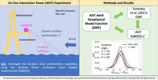
2.1. KaBODS Instrument Description

The KaBODS scatterometer is a Ka-band vertically polarized Frequency Modulated Continuous Wave (FMCW) radar. It was located on the main platform of the ASIT at 13.1 m above the mean sea level. This platform pointed toward 245° (clockwise) relative to the true North. The KaBODS radar has two standard gain pyramidal horn antennas, one of which is used to transmit while the other is used to receive. Each antenna has a boresight angle of 60°. Through range compression, the radar collects measurements at different incidence angles, ranging between 20° and 83°. Originally, both the transmit and receive antennas were configured to be in vertical polarization (VV). On 20 November 2020, a strong wind event rotated the receiving antenna by 45°, allowing a configuration in vertical–horizontal polarization (VH). Given the small value of the cross-polarized return from the ocean at low to moderate wind speed, we do not expect that these returns will corrupt our co-polarized estimates significantly. Yurovsky et al. [24] showed that the predicted errors associated to a cross-polarized contamination are small for wind speeds lower than 25 m/s, particularly for the VV return. Therefore, in line with these results and considering that the range of wind speeds used in this work does not exceed 18 m/s, we decided to ignore the VH contribution. In addition, the data before and after the polarization switch are consistent.

The system details are presented in

Table 1. KaBODS key system characteristics.

Name	Value
Bandwidth	100 MHz
Pulse Repetition Frequency	1 kHz
Sample number per pulse	391
Transmit power	9 dBm
Antenna peak gain	23.58 dB
Boresight angle	60°
H-Plane antenna aperture width	68.88 mm
E-Plane antenna aperture width	52.37 mm
3 dB Azimuth Beamwidth	10°
3 dB Elevation Beamwidth	10°
Platform Altitude	13.1 m
Range Resolution	1.5 m
Elevation Resolution	1.6–4.4 m

. With a bandwidth of 100 MHz, the radar range resolution, which represents the radar’s ability to distinguish between targets, is ∼1.5 m, which is sufficient to resolve surface waves. At the Ka-band radar frequency, the radar is sensitive to Bragg surface wave components of ∼0.8 cm wavelength [2].

The KaBODS radar amplitude measurements were calibrated with calibration targets deployed at various ranges in the far field. The system did not have an internal calibration gain loop, so transmit power variations, due to temperature, for instance, were not corrected, leading to potential uncertainty in the absolute value of the radar cross section, but with a lesser impact on the study of azimuth and angular modulations, since these are relative measurements collected under the same environmental conditions. We note, however, that our absolute calibration is largely consistent with the results reported in [24].

The KaBODS azimuth look direction is controlled by a motor which allows the radar to steer in azimuth with about 160° range. The radar collects continuous data at each azimuth location for five minutes with a collection cycle of one hour. An example of the nominal KaBODS azimuth positions within a one-hour cycle is shown in Figure 1. The KaBODS dwell time and configuration were set to maximize the KaBODS time within the footprint of a polarimeter, which was installed on the ASIT. This results in a longer dwell time at the radar azimuth position of 203°, as shown in Figure 1.

For this study, we used KaBODS L0 products from October 2019 to January 2020. The L0 products contain the Single Look Complex (SLC) radar data, as a function of time and radar range, as well as the radar azimuth position relative to the normal of the ASIT platform.

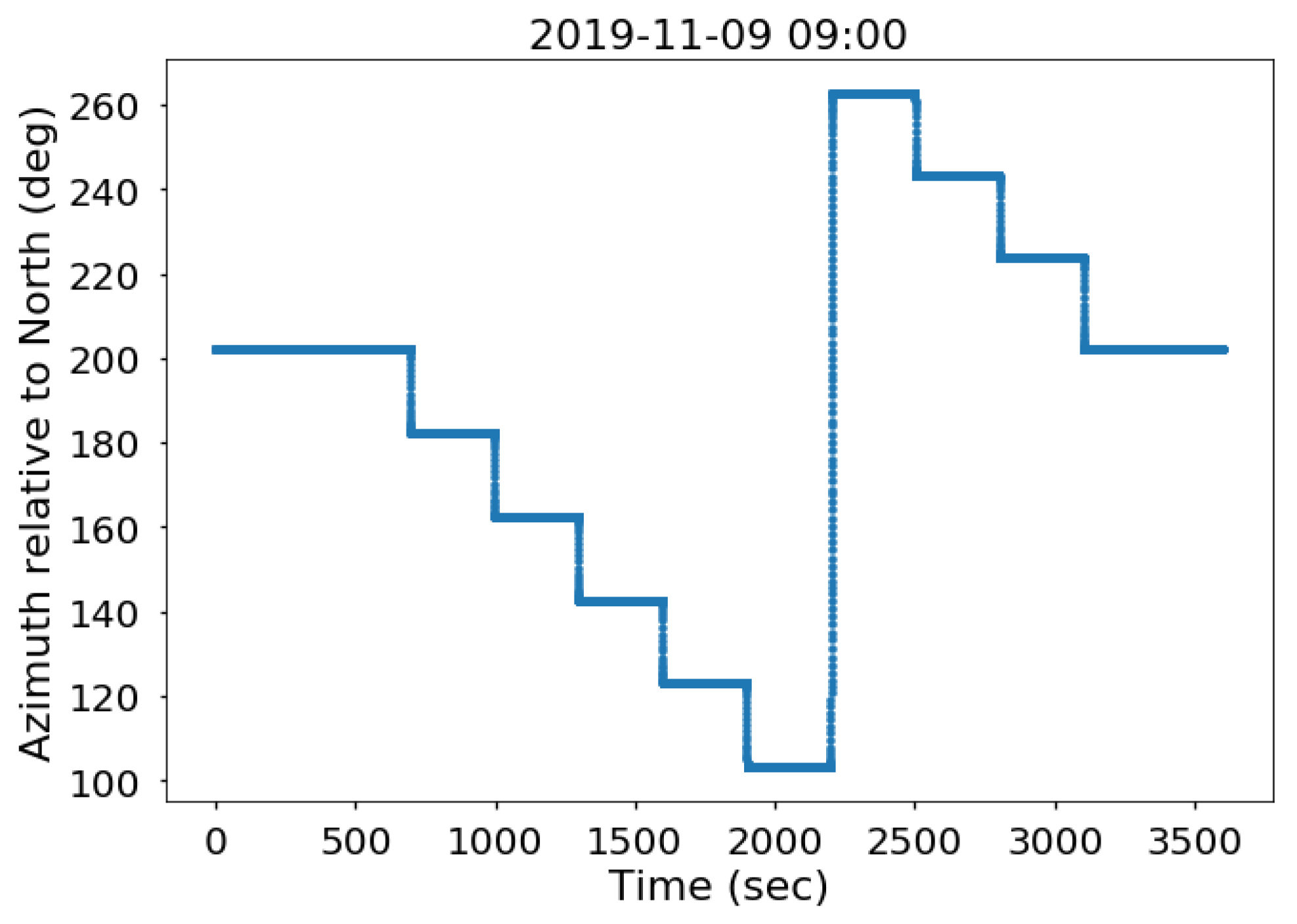
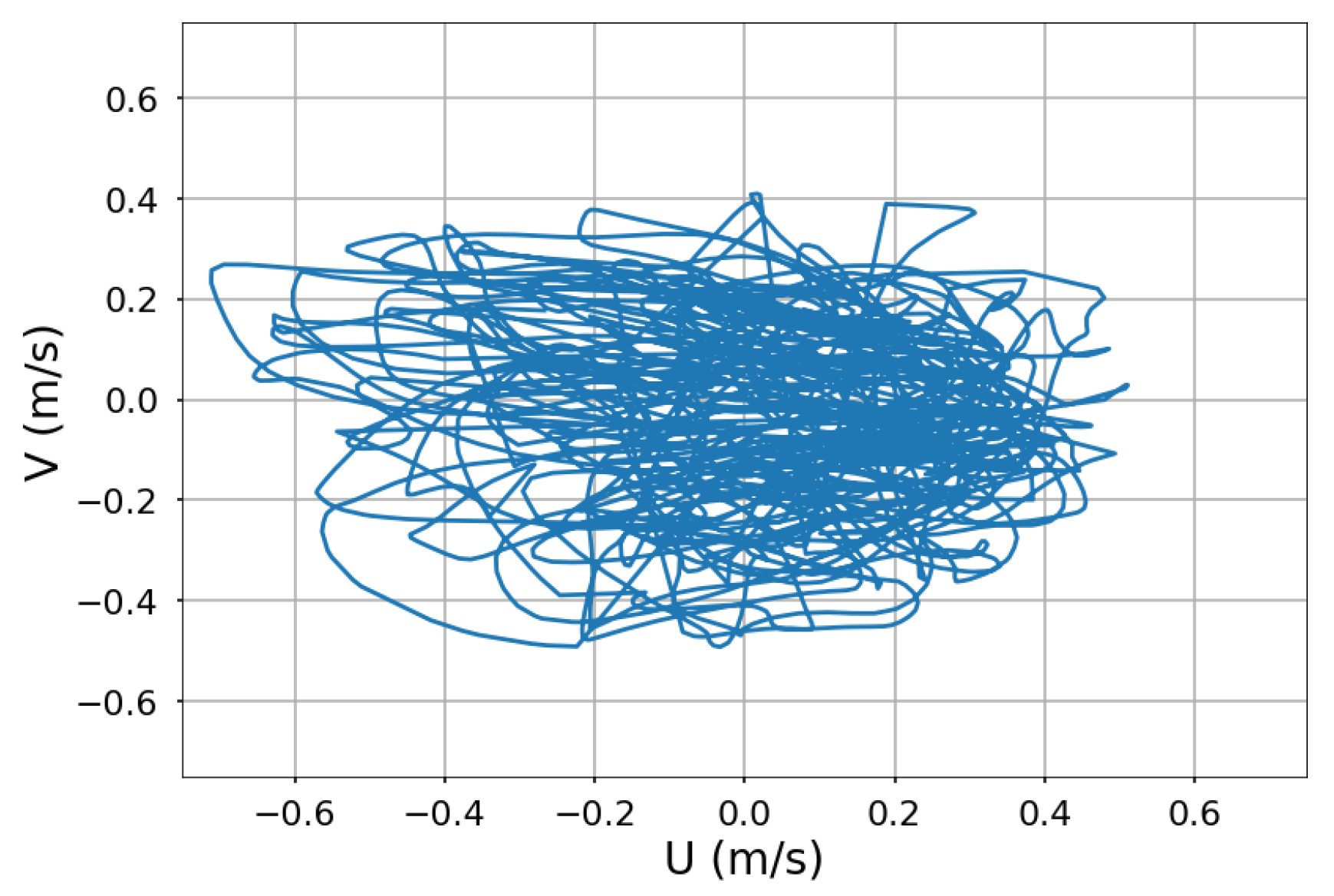
2.2. Meteorological and Oceanic Data Collection

The wind measurements used in this study were obtained from six sonic anemometers located on the ASIT at different heights. Three anemometers are located on the ASIT Rohn Tower, above the main platform, between 12 and 23 m. The other three anemometers were located on the ASIT mast extending off the end of the main platform. A description of the ASIT instruments with their corresponding location can be found in [27,31]. The wind measurements were converted to a common height of 10 m using the Coupled Ocean–Atmosphere Response Experiment (COARE) bulk algorithm version 3.5 [31]. The measurement heights were adjusted to account for changes in the sea surface height relative to the ASIT, mainly due to tides. To develop the ASIT GMF, we used these 10 m winds, relative to water, adjusted for neutral conditions, known as equivalent neutral wind [31]. To compute the wind speed relative to water, the surface currents available from the Acoustic Doppler Current Profiler (ADCP) located nearby the ASIT were used. The distribution of the equivalent neutral wind speed ($U{10}_N$) and wind direction relative to the radar azimuth (given in meteorological convention) ($\varphi$) is shown in Figure 2a,b, respectively. During the experiment, a wide range of wind intensities was encountered, between 1–18 m/s, with the majority of the data ranging between 5–8 m/s. As noted before, thanks to the radar’s capability of scanning in the azimuth direction, the data set covers a wide range of relative wind-radar boresight azimuth directions.

For this study, in addition to the wind measurements, we also had measurements of the sea surface temperature (SST), the dominant wave period ($T_{peak}$), the significant wave height ($H_s$) and the precipitation rate ($P_r$) (Figure 2c–f). $T_{peak}$ represents the period of the most energetic ocean wave component, whereas $H_s$ represents the mean height of the highest one-third of the waves [32]. These parameters have been used to filter out the backscatter data that can potentially be compromised by rain, as well as environmental conditions where insufficient data were available for a reliable result. Hereafter, we use only KaBODS data corresponding to $T_{peak}$ < 10 s, $H_s$ < 2.5 m and rain rate <1 mm/h. As can be seen from Figure 2, this only excluded a relatively small number of observations.

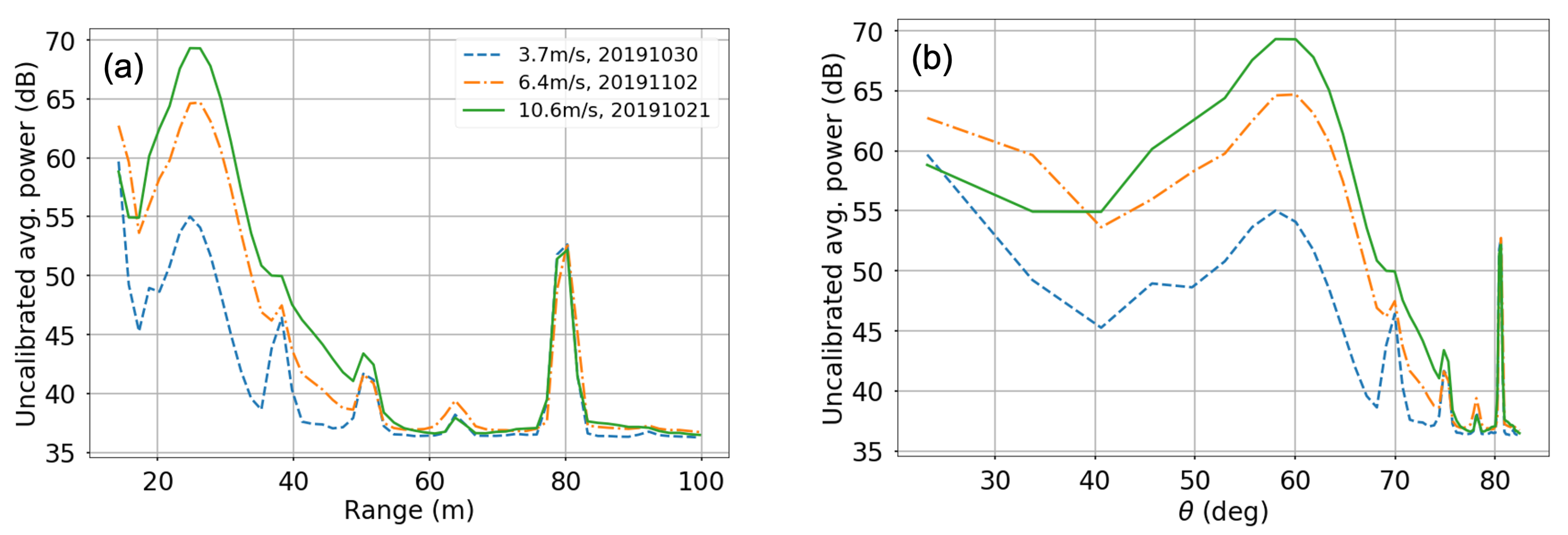
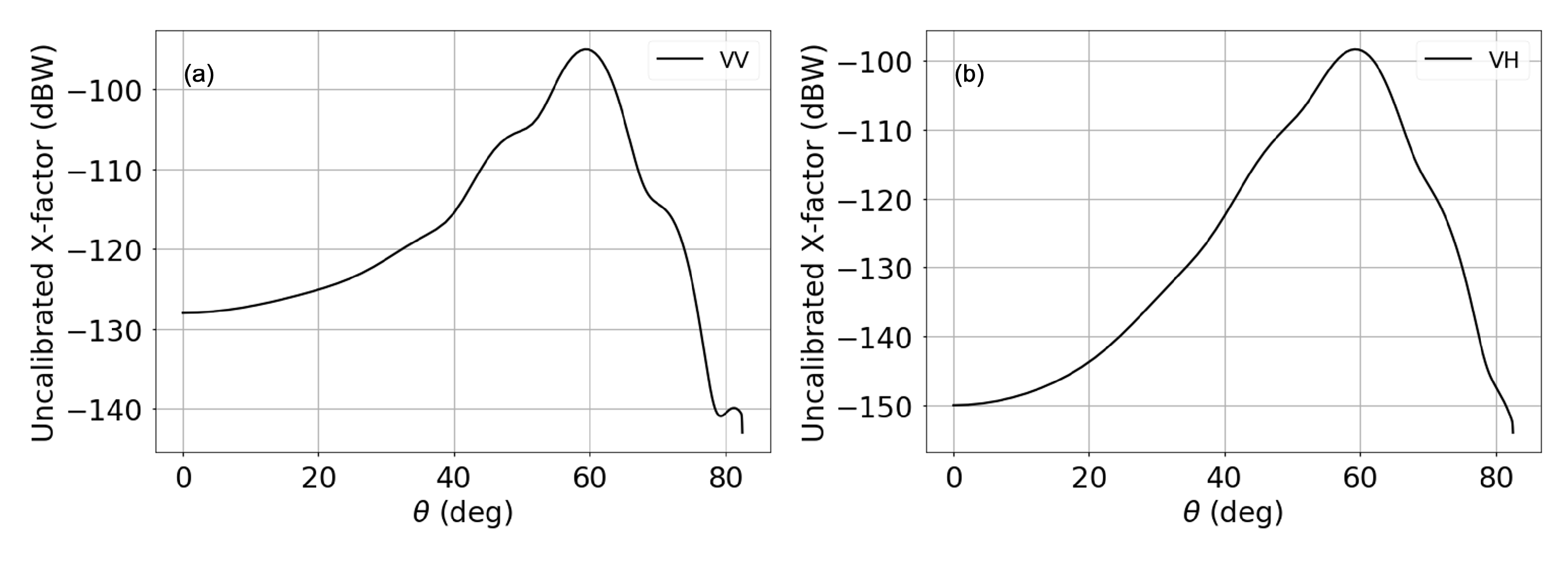
2.3. KaBODS Signal Power Processing

The KaBODS total return power was computed as the magnitude squared of the SLC data, corrected with a calibration constant, as described below. Two major contributions affect the return power, namely, the speckle noise and the thermal noise. Speckle noise is the result of random phase variations in the interaction between the radar signal and the ocean surface [33]. Such phase variations are mainly introduced by the small-scale properties of the surface, the random motion of the point scatters and the variation of the distance between the radar and the point-target. In order to reduce the speckle noise, a multi-looking approach is usually used, averaging independent samples (looks). To this end, we have averaged the KaBODS received power over $N_L$ = 50 looks (radar pulses), that results in averaging over 50 ms. The resulting cross section speckle is reduced by a factor of approximately $10{log}_{10}\left(1+N_L^{-1/2}\right)\approx 0.6$ dB for each 50 ms measurement. After averaging for 5 min, the estimated speckle variability (not including geophysical variability) would be in the order of ∼$0.06$ dB.

The thermal noise power comes from the instrument itself and it introduces a bias in the return power [34]. It is dependent on the system temperature and its bandwidth. Figure 3a and b show the KaBODS multi-looked return power as a function of the radar range and incidence angle, respectively. Three different days/times are shown, corresponding to three different wind speed values, 3.7 m/s, 6.4 m/s and 10.6 m/s. As expected, the power increases as the wind speed increases. However, at ranges higher than 86 m, corresponding to incidence angles greater than 82°, the power does not change with the wind intensity, it appears rather constant, suggesting the presence of a noise component. Therefore, we have estimated the value of the KaBODS thermal noise by averaging the multi-looked power starting at an incidence angle of 82°. We then computed the power associated only with the signal (echo), by subtracting the thermal noise component ($P_N$) from the total return power ($P_r$) [34]:

$$P_s=P_r-P_N$$

(1)

An important aspect shown in Figure 3 is the presence of spikes in the KaBODS return power at ranges of 14.25 m, 38.25 m, 50.25 m, 63.75 m and 80.25 m (Figure 3a), corresponding to incidence angles of 23.18°, 69.97°, 74.89°, 78.14°, and 80.60° (Figure 3b), respectively. These peaks are not significantly affected by the wind speed and they are probably due to a RF-leakage from either the KaBODS system itself or the other instruments on the ASIT, rather than an effect from the ocean surface. Therefore, in this paper, we focus only on the range between 17 m and 35 m, i.e., between 40° to 68°, to avoid possible instrument contamination.

Figure 4 shows the KaBODS signal-to-noise ratio (SNR) as a function of the incidence angle for different wind speed ranges. The SNR shows a maximum around 60°, which is consistent with the radar look angle and main lobe of the antenna pattern. It also shows a second peak between 45° and 50°, coincident with an antenna side lobe. Additional details on the antenna pattern are given in Section 2.4.

2.4. The KaBODS Surface Backscatter Computation

In order to convert the signal power $P_s$ into the corresponding ocean surface radar backscatter (σ°) we have used the radar equation as shown in (2):

$$P_s={\sigma }^{\circ }X{K}_{cal}$$

(2)

where $K_{cal}$ is a radar calibration constant (computed using known corner reflectors) and X is the X–factor. The X–factor is a pre-computed constant that is needed to convert measured return power into ocean surface backscatter. It accounts for both the radar geometry and the antenna pattern. We have modeled the X–factor as shown in (3).

$$X\left(r_0\right)=\frac{{\lambda }^2{P}_t}{{\left(4\pi \right)}^3}\int \int \frac{1}{r^4}{G}_t(\theta ,\alpha )G_r(\theta ,\alpha ){\chi }^2(r-r_0)d\alpha dr$$

(3)

where $P_t$ is the transmitted power, $G_t(\theta ,\alpha )$ and $G_r(\theta ,\alpha )$ are the receive and transmit antenna gains as function of elevation $\theta$ and azimuth $\alpha$, respectively. The KaBODS antenna patterns were not calibrated independently, but, since they are commercial standard gain horns used for calibration, their pattern as a function of angle is well known and within the tolerances for this study. The term $\chi (r-r_0)$ represents the point-target response (PTR), as a function of the range r centered at $r_0$. The definition of $\chi$ depends on the radar processing of the received signal from a point target. As an FMCW radar, the KaBODS transmits a signal that is frequency-modulated. This allows for pulse compression on the received signal, which is a signal processing technique usually used to improve the radar range resolution as well as the signal-to-noise ratio [1]. However, this technique also enhances the presence of the side lobes in the received compressed pulse in the time domain. These side lobes are in addition to the main pulse from the target and weighting functions are used to reduce their amplitude [35]. For the the KaBODS system, a Hanning weighting function has been used to produce the SLC measurements. Therefore, $\chi$ is defined as a Hanning-weighted PTR. Two different configurations of the X–factor were implemented to account for both VV and VH-polarizations, in order to be consistent with the received antenna rotation configuration. The resulting X–factor as a function of the incidence angles for both VV and VH polarization is shown in Figure 5. Here, we show the X–factor for the whole range of incidence angles available from the KaBODS system. The peak corresponding to the antenna pattern main lobe is located at 60°, whereas two side lobes are located between 45–50° and 70–75°. This X–factor model is consistent with the KaBODS power shown in Figure 3b. It also shows that the power spike seen at 23° does not correspond to a sidelobe of the antenna pattern. The spikes seen at 70° and 75° appear to be caused by the energy entering through the sidelobe of the antenna pattern. However, since the power does not significantly change with the wind, we believe that those angles should be excluded from the analysis.

The KaBODS calibration constant $K_{cal}$ characterizes the radar system and its estimation is essential in correctly computing ${\sigma }^0$ from the received signal. The KaBODS system was calibrated on the ground by use of the three corner reflectors placed at 12 m, 26 m and 40 m distance from the radar, as described in [36]. These reflectors have a known radar cross section, so that by recording the received power and measuring the transmitted power, the calibration constant can be estimated. The estimated $K_{cal}$ value of the KaBODS system is 182.8 dBW and we have used this value in the data processing.

The measured data were processed to estimate the corresponding ${\sigma }^0$ measurement. We performed a quality check of the obtained ${\sigma }^0$ time series and we found cases with ${\sigma }^0$ spikes exceeding 0 dB. Each spike was visible at different incidence angles and according to the anemometer winds, they were associated with low wind speed conditions. This suggests that such high backscatter values were likely due to particular events happening at the sea surface (e.g., boats), within the radar footprint, rather than wind/wave effects. For this reason, we decided to filter out values of ${\sigma }^0$ higher than −5 dB, to exclude corruption of measurements by bright targets.

An additional mechanism which can also increase the variability of the surface backscatter at the spatial resolution of the KaBODS system is the modulation induced by the long waves. Additional details on the wave-induced backscatter modulation are given in Section 4. The variability caused by large wave modulation is inherently present in large-footprint spaceborne scatterometer measurements. Since we want our results to be applicable to this situation, we replace spatial averaging with temporal averaging, we averaged the surface backscatter over the azimuth dwell. This corresponds to averaging over a time period of about five minutes: this corresponds to spatial averaging over ∼1.6 km to ∼2.6 km for waves ranging between 20 m and 50 m, which is comparable to spaceborne spatial scales. Each averaged ${\sigma }^0$ value (hereafter, <${\sigma }^0$>) was then associated to the azimuth mean of the corresponding azimuth subset and it has been collocated with the anemometer measurements. This collocated data set was then used for the GMF development.

2.5. Geophysical Model Function Development

We derived the ASIT GMF as a function of the radar incidence angle ($\theta$), the 10 m equivalent neutral surface wind speed ($U{10}_N$) and the wind direction relative to the radar azimuth ($\varphi$), by using the functional form as a described in Yurovsky et al. [24], as shown in (4).

$$log{\sigma }^{\circ }=A_0(\theta ,U{10}_N)+A_1(\theta ,U{10}_N)cos\left(\varphi \right)+A_2(\theta ,U{10}_N)cos\left(2\varphi \right)$$

(4)

where the $A_i$ coefficients are presented as functions of $\theta$ with a dependence on $logU{10}_N$:

$$A_i=\sum _{m=0}^4\sum _{k=0}^1{c}_{mik}{\theta }^m{(logU{10}_N)}^k$$

(5)

To build the GMF, we derived the $c_{mik}$ coefficients by mapping the KaBODS $<{\sigma }^0>$ measurements to the collocated anemometer wind speeds and directions. We used a least-squares fitting method with a Cauchy loss function to weaken the influence of possible outliers. The ASIT anemometer array and ancillary instruments have the large advantage that wind stress can be calculated and converted to an estimate of neutral winds at 10 m [31], and we use these to construct our GMF. We noticed that the functional form given in (4) does not fit well over a large range of wind speeds. In particular, the surface backscatter at very low wind speeds tends to drop faster than the prescribed log parameterization [37]. Therefore, we excluded measurements at wind speeds lower than 3 m/s, in favor of a good fit for moderate and higher winds. With respect to the wind direction, we noticed that the ASIT is a point of distortion for the KaBODS backscatter measurements when the wind is blowing away from the radar. These data correspond to a wind direction of 180° relative to the radar azimuth (downwind direction). This distortion is due to the fact that the ASIT shadows the water surface, affecting the surface roughness. Therefore, given the few degrees of freedom of the fitting model, we have decided to exclude from the training data set the backscatter measurements with a relative wind direction within 30° from the downwind direction, in favor of a good fit up to 150°, which is known to be free from shadowing effects. Moreover, the radar position on the ASIT main platform causes the radar beam, with the azimuth direction of ∼262° (relative to the true North), to point into the main platform. This results in contaminated backscatter measurements which have also been excluded from the analysis. The values of the obtained ASIT GMF coefficients ($c_{mik}$) are shown in Appendix A.

3. Results

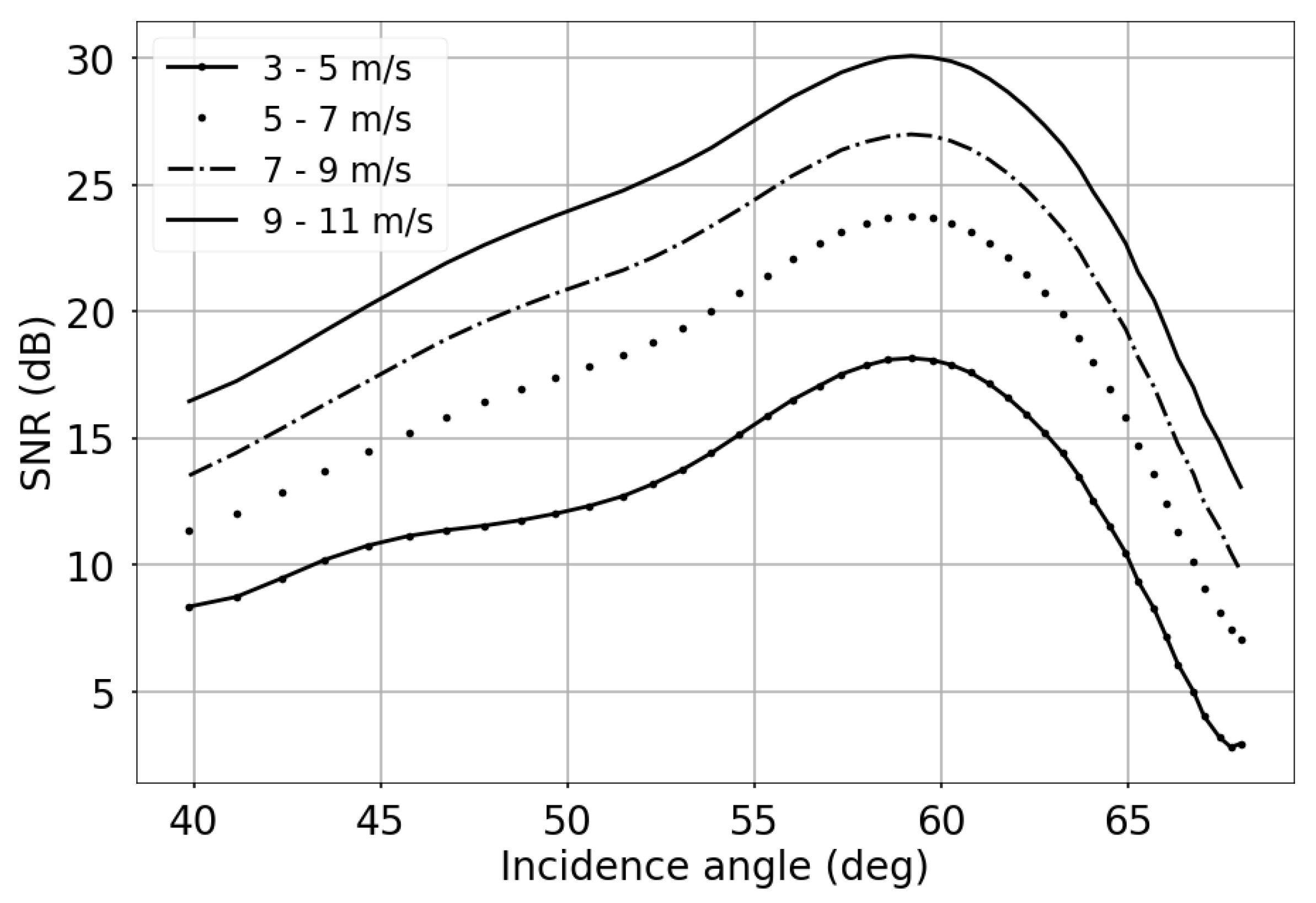
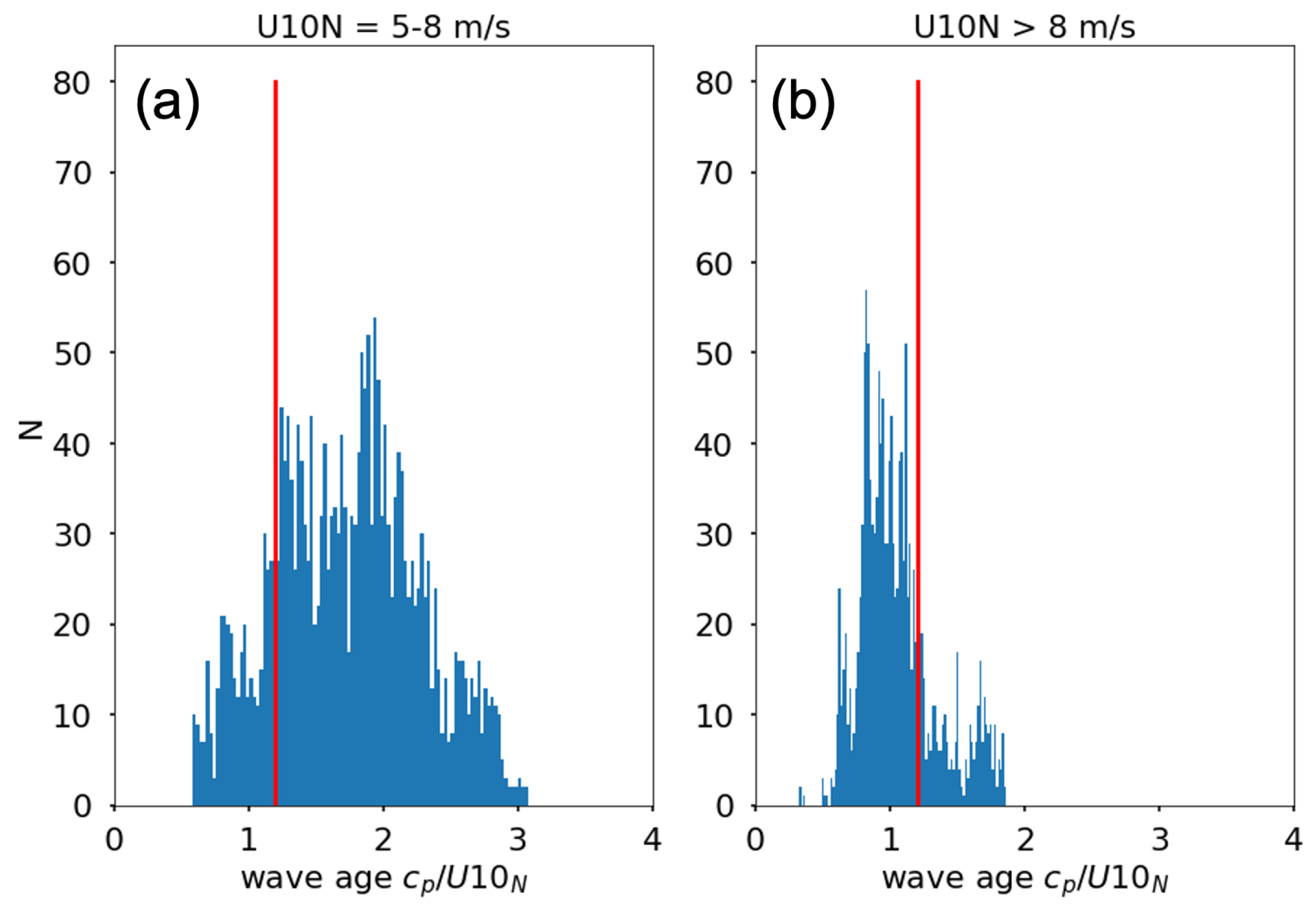
3.1. Wind Speed Sensitivity

We first analyzed the sensitivity of the KaBODS backscatter with respect to the wind speed and compared results for the ASIT GMF with the KaDPMod GMF. Figure 6 shows the KaBODS <σ°> binned over 1 m/s range (blue dots with error bars) along with the ASIT GMF (solid orange line) and the KaDPMod GMF (dashed black line) as a function of the wind speed. The results are shown for $\varphi =0^{\circ }$ (upwind), $\varphi ={90}^{\circ }$ (crosswind), $\varphi ={150}^{\circ }$ and $\varphi ={180}^{\circ }$ (downwind), at three different incidence angles, 40°, 50° and 60°. The KaBODS measurements are modulated by the wind speed and the ASIT GMF is able to describe this wind sensitivity with a residual absolute mean bias (${\mu }_{ASIT}$) ranging between 0.15 dB to 0.95 dB and a residual standard deviation (${\sigma }_{ASIT}$) between 1.96 dB and 3.17 dB for relative wind directions up to 150°. These values were calculated as the mean bias and the standard deviation of the differences between the model and the actual measurements in log space. In downwind direction, the agreement between the ASIT GMF and the measurements is not as good as at 150°. This could be ascribed to the fact that the ASIT GMF has not been trained at this angle, as explained in the previous section. However, this could also be an indication of the potential shadowing effects. In addition, a disagreement is observed for wind speeds higher than 12 m/s, mostly due to the lack of data used to train the GMF at high wind speed conditions.

Overall, the KaDPMod and the ASIT GMF are consistent, however, the KaDPMod describes a slightly different wind speed sensitivity with respect to the KaBODS backscatter and in turn to the ASIT GMF. The residual absolute mean bias (${\mu }_{Y16}$) ranges between 0.43 dB to 3.63 dB with a mean standard deviation (${\sigma }_{Y16}$) ranging between 2.05 dB to 3.22 dB. The values of ${\mu }_{Y16}$ are higher compared to ${\mu }_{ASIT}$. This is expected since the ASIT GMF is built by fitting the data. Notice that these differences vary with wind speed and incidence angle, and cannot be ascribed to an overall calibration difference between the two system: in general, the absolute calibration seems consistent between the two data sets. The ${\sigma }_{Y16}$ values are mostly consistent with the ${\sigma }_{ASIT}$ values for different relative wind directions and incidence angles. An offset is seen between the KaDPMod and the ASIT GMF at 40°, particularly in the upwind and crosswind directions and this offset decreases at higher incidence angles.

3.2. Wind Direction Modulation

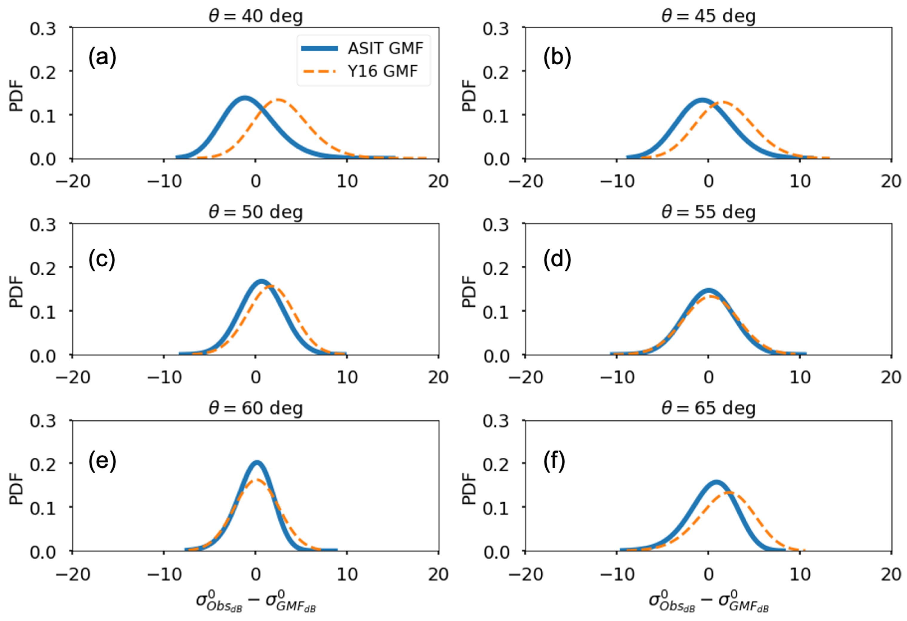
Figure 7 shows the KaBODS surface backscatter with respect to the relative wind direction, at wind speeds of 5 m/s (left), 7 m/s (middle) and 9 m/s (right). The dots and error bars represent the mean with the corresponding standard deviation of the KaBODS backscatter binned over 10°-direction. To this end, at a given incidence angle, firstly we binned the data over 1 m/s bin centered at 5, 7 and 9 m/s. Bins of 1 m/s are used to ensure enough data points. Each wind speed bin was then sorted in 10°-direction bins where the corresponding backscatter mean and standard deviation were computed.

The KaBODS backscatter shows a clear modulation with the wind direction and as expected, the ASIT GMF is able to reproduce such modulation with a relatively low absolute value of ${\mu }_{ASIT}$ ranging between 0.09 dB to 0.96 dB and ${\sigma }_{ASIT}$ between 2.16 dB to 3.71 dB. The KaBODS backscatter shows a stronger directional modulation at an incidence angle of 50° and 60° than 40°. Indeed, as also described by the ASIT GMF, the directional modulation tends to be smoother at 40°, regardless of the wind intensity.

The comparison between the KaDPMod and the ASIT GMF shows that the KaDPMod GMF does not fully describe the directional modulation of the KaBODS measurements. At 50°, the KaDPMod GMF shows a slightly smoother modulation compared to the ASIT GMF and the KaBODS data. This effect worsens at 60°. This uncertainty in the KaDPMod GMF directional modulation can be ascribed to the data used to train this GMF [17]. Due to the nature of the Black Sea tower measurements, the collected data set did not have a wide azimuth variability and this may have affected the model sensitivity with respect to the relative wind direction. In our setup, nearly co-temporaneous azimuth variability was guaranteed by completing azimuth cycles within one hour.

The KaDPMod residuals absolute mean bias ${\mu }_{Y16}$ ranges between 0.08 dB to 3.25 dB and the standard deviation ${\sigma }_{Y16}$ between 2.48 dB to 3.77 dB. As for the wind speed sensitivity, the models show an offset at 40°, with an incidence angle dependence, but they show similar values of the residuals mean standard deviations for different wind speeds and incidence angles.

3.3. Model Accuracy

In order to further evaluate the accuracy of both models with respect to the KaBODS <${\sigma }^0$> data, we computed the statistics of the model residuals for the whole data set along with the root mean square difference and the correlation coefficient. The distribution of the model residuals is shown in Figure 8. The analysis is carried out for a range of incidence angles: 40°, 45°, 50°, 55°, 60° and 65°. The results are shown in

Table 2. The mean bias ($\mu$ dB) and the mean standard deviation ($\sigma$ dB) of the residuals of both the ASIT GMF and the KaDPMod from Yurovsky et al. along with the root mean square difference ($\epsilon$ dB) and the correlation coefficient (R).

$\mathit{\theta }$	${\mathit{\mu }}_{\mathit{A}\mathit{S}\mathit{I}\mathit{T}}$	${\mathit{\mu }}_{\mathit{Y}}$	${\mathit{\sigma }}_{\mathit{A}\mathit{S}\mathit{I}\mathit{T}}$	${\mathit{\sigma }}_{\mathit{Y}}$	${\mathit{\epsilon }}_{\mathit{A}\mathit{S}\mathit{I}\mathit{T}}$	${\mathit{\epsilon }}_{\mathit{Y}}$	${\mathit{R}}_{\mathit{A}\mathit{S}\mathit{I}\mathit{T}}$	${\mathit{R}}_{\mathit{Y}}$
40°	−0.55	+2.93	+3.01	+3.08	+3.05	+4.25	+0.71	+0.69
45°	−0.37	+1.80	+3.00	+3.11	+3.02	+3.60	+0.76	+0.75
50°	+0.69	+1.63	+2.37	+2.55	+2.47	+3.02	+0.85	+0.84
55°	+0.03	+0.24	+2.71	+2.99	+2.71	+3.00	+0.83	+0.81
60°	−0.16	+0.14	+2.03	+2.45	+2.04	+2.45	+0.88	+0.86
65°	+0.34	+1.81	+2.59	+3.01	+2.61	+3.52	+0.83	+0.78

. Overall, both models appear well correlated with the data, with a correlation coefficient ranging between 0.71 and 0.88 for the ASIT GMF and 0.69 to 0.86 for the KaDPMod. As expected, the ASIT GMF better agrees with the KaBODS <${\sigma }^0$> measurements then KaDPMod, as shown by lower values of the mean bias. We note that these statistics show a trend with incidence angle. In particular, they tend to improve at 60°, where we observe the lowest values of mean bias, standard deviation, root mean square errors and the highest correlation. However, they tend to worsen again at 65°. This particular dependence on the incidence angle could be related to the shape of the antenna pattern. However, because the SNR is high over the whole incidence angle range, these results may also suggest that the surface wave components that better respond to the Ka-band radar are those observed at (and close) an incidence angle of 60°. It is interesting to notice that the offset between the ASIT GMF and the KaDPMod also shows a similar trend, as it tends to disappear at 60° (Figure 8). The nature of such incidence angle dependence is currently under investigation.

Both models show a residual distribution that is Gaussian in log-space. It is interesting to see that, consistent with the two previous analyses, the standard deviation values do not significantly change between the two models when using the whole data set to compute the residuals. We believe that such variability is not related to the model accuracy, but rather to a backscatter variability that is not fully captured by the parameterization. Since we have processed the data to reduce the modulation due to the speckle and thermal instrument noise, we believe that such variability has a geophysical source.

4. Discussion

Based on the results of the model residuals, our main focus has been understanding the source of the observed residual backscatter variability.

As mentioned in Section 2.2, we used the winds as water-relative, i.e., corrected by the surface currents available from the ADCP. We also performed the same analysis using the earth-relative winds, but no significant difference was seen as we obtained very similar results. This is due to the fact that the typical currents on the site were lower than 30–50 cm/s, which is much smaller than the wind speeds encountered during the experiment. Figure 9 shows the values of the velocity components obtained by the ADCP. Therefore, this suggests that possible effects due to the surface currents on this site are expected to be small.

An important source of the Ka-band backscatter modulation at moderate and high incidence angles, is hydrodynamic modulation [38]. This phenomenon is caused by the backscatter modulation induced by the long waves. This occurs since the short wave components, locally generated by the wind, are modulated by the long wave orbital velocity [39]. These long waves are usually generated further away, but they propagate into the observed scene and are referred to as swell [32]. According to Yurovsky et al. [38], the backscatter modulation due to long waves tends to decrease as the wind speed increases. As explained in Section 2.3, to account for the effect of the long-wave modulation, we averaged the backscatter over the azimuth dwell time of about five minutes. However, a residual variability could still be associated with longer period waves, where 5 min may not be sufficient to average out their contribution. Therefore, to further assess the impact of the wave-induced modulation, we computed the wave age as $c_p/U{10}_N$, where $c_p$ is the phase velocity of the wave component with period $T_p$ [40]. The wave age represents a measure of the wave development status and we used it to identify swell-dominated data [31]. In particular, we used a wave age value of 1.2 to identify the data corresponding to fully developed sea, which is the condition of equilibrium between the wave energy source and dissipation. Wave age values greater than 1.2 identify decaying seas dominated by swell, whereas values of less than 1.2 represent developing seas [31]. As shown in Figure 10, the majority of the ASIT data with wind speed between 5–8 m/s fall under swell conditions. We then computed the model residuals by filtering the data with wave age higher than 2.2, in order to reduce the amount of swell-contaminated data. The results show that the standard deviation of the model residuals does not significantly change. We also used different wave age thresholds, such as, 2, 1.8 and 1.6 to filter the data. However, we observe that even when filtering a larger amount of swell-contaminated data, the standard deviation is not significantly reduced. This suggests that the long-wave modulation is not the primary source of the KaBODS residual backscatter variability. Similar results were also obtained by performing the same analysis over data points within easterly and south-westerly wind directions to provide long fetches and resemble open-ocean conditions.

Past works have shown the importance of including the sea surface temperature (SST) in the Ku-band geophysical model function in order to improve the accuracy of wind retrieval from scatterometers [13]. The SST can modify the roughness of the surface through modification of the surface water viscosity [41]. It has also been shown that SST perturbations affect the wind stress field through the stability of the marine atmospheric boundary layer [42,43]. Vandemark et al. [12], showed that the ocean backscatter at Ka-band for incidence angles near nadir and at low wind speeds varies between cold and warm water. The SST is also expected to have an impact at larger incidence angles. As shown in Figure 2, the SST during the ASIT experiment covered a range between 4 °C to 14 °C. Therefore, in line with these previous studies, we analyzed the averaged KaBODS backscatter with respect to the SST for low-medium wind speed. However, at the KaBODS spatial resolution, we have not found a clear signature of an SST contribution to the observed residual variability. Given the uncertainty in the radar gain as a function of temperature, and the weakness of the observed signal, we are not confident in concluding anything definite at this stage and leave this for future research.

One feature that we observe in the KaBODS backscatter data set is that the KaBODS time series (i.e., the measurements before averaging over the azimuth dwell period) show a spiky structure. As a consequence of this structure, the backscatter distribution is not Gaussian, but rather skewed in linear space. Figure 11a shows the backscatter time series at an incidence angle of 60°, for two different days/times in similar wind conditions, corresponding to wind speed between 8–9 m/s, in the upwind direction and in the absence of swell. The blue trace shows an example of the typical KaBODS backscatter spiky structure, with the corresponding distribution (Figure 11b). In this case, the distribution skewness is 1.50. We found that in presence of spikes with a magnitude much larger than the background backscatter, as shown from the red trace, the value of the distribution skewness significantly increases. For this case, the skewness increases from 1.50 to 5.46. Similar results are obtained at different wind speed conditions, as shown in Figure 11c,d, for a wind speed between 6–7 m/s. In this case, the skewness increases from 1.45 to 4.3. Yurovsky et al. [44] suggested that the presence of high amplitude spikes, making the distribution strongly skewed in linear space, is likely due to wave breaking events. In particular, they showed that at moderate to high incidence angles, these backscatter spikes represent a non-negligible non-polarized backscatter component associated to quasi specular reflection from breaking facets. Although the contribution of this non-polarized component is shown to be stronger at horizontal polarization than vertical polarization [44], such spikes are also visible in vertical polarization, as shown in [45], and they can also be associated to enhanced roughness of the ocean surface from post wave-breaking events, as described in [46]. Moreover, although the studies of wave breaking effects usually focus on moderate to high wind speed conditions, it was suggested in [38] that the capillary waves observed at Ka-band at low wind speed conditions are generated as parasitic capillary waves from the breaking of short-gravity waves [3], showing a possible breaking contribution at low winds as well. Therefore, in line with these studies, we believe that the large spikes observed in the KaBODS backscatter show a contribution due to wave breaking effects. Further investigations are now ongoing to fully characterize the observed spiky structure as well as the impact that the wave breaking events have on the KaBODS backscatter distribution.

5. Conclusions

In this work, we present a Ka-band wind geophysical model function based on the data collected during the WHOI ASIT experiment. The ASIT was equipped with a Ka-band Doppler scatterometer along with six sonic anemometers, allowing direct estimation of neutral winds and providing a unique data set with collocated ocean surface backscatter and wind measurements.

The ASIT GMF has been compared to the existing KaDPMod GMF, which was developed from measurements taken during a different tower experiment conducted over the Black Sea. We have analyzed the two GMFs with respect to the wind speed and relative wind direction and we have analyzed the accuracy of both models with respect to the KaBODS data set. Both GMFs are well correlated with the data, with a correlation coefficient ranging from 0.7 to 0.9. The correlation coefficient values are slightly larger with the ASIT GMF than the KaDPMod. This is expected by construction since the ASIT GMF was trained using the data. However, the KaDPMod shows a slightly different sensitivity to the wind speed and a smoother directional modulation than the ASIT GMF, particularly at larger incident angles (>50°). We believe that the KaDPMod smoother modulation is probably due to the fact that the data used to train the model was sparse in terms of azimuth variability and this may have affected the accuracy of the KaDPMod directional component.

We also observe that the two GMFs have a consistent residual variability that we concluded as being mainly associated with a variability of the surface backscatter. To analyze this residual backscatter variability with respect to the long-wave induced modulation we have taken into account the wave age parameter and we concluded that this modulation is not the primary source of the observed variability. We have also analyzed the possible effect associated to the SST, however, we could not see, at this stage, a clear signature associated with the SST variation at the spatial resolution of the KaBODS system. One feature that we observe is that the surface backscatter has a spiky structure and the presence of spikes with magnitude greater than the background makes the distribution of the backscatter strongly skewed in linear space. Such results are consistent with what has been observed in previous studies, suggesting the presence of a contribution due to wave breaking events.

Moreover, we observe that the statistics of both models as well as the backscatter residual variability show a trend with the incidence angle. They tend to significantly improve at an incidence angle of 60°. Although the KaBODS antenna has a peak gain at 60°, it is worth noticing that the SNR is high within the whole incidence angle range, and the variability is a relative measurement over a short time, and not expected to be affected by the absolute gain. Therefore, the observed trend may indicate that the wave components observed at an incidence angle of 60° (and closer) are those that better respond to the Ka-band frequency in terms of wind interaction, according to the Bragg scattering mechanism.

The results of this work show that the ASIT data set is extremely valuable as a reference data set for investigations of new and existing GMFs at Ka-band. The results of the comparison of the GMFs with the actual data provide guidance for future efforts to fully characterize the surface backscatter mechanisms at Ka-band. We are currently investigating the impact of the incidence angle in order to explore the optimal viewing geometry for future mission design. We are also analyzing the potential signature of breaking waves in the surface backscatter distribution and the possible SST effects.

References

1. Ulaby, F.T.; Long, D.G. Radar Measurements and Scatterometers. In Microwave Radar and Radiometric Remote Sensing, 4th ed.; The University of Michigan Press: Ann Arbor, MI, USA, 2014; pp. 605–669. [Google Scholar]
2. Valenzuela, G.R. Theories for the Interaction of Electromagnetic Waves and Oceanic Waves. A Review. Bound. Layer Met. 1978, 13, 61–85. [Google Scholar] [CrossRef]
3. Kudryavtsev, V.N.; Hauser, D.; Caudal, G.; Chapron, B. A Semiempirical Model of the Normalized Radar Cross-Section of the Sea Surface 1. Background model. J. Geophys. Res. Oceans 2003, 108, C08054. [Google Scholar] [CrossRef] [Green Version]
4. Hersbach, H.; Stoffelen, A.; de Haan, S. An Improved C-band Scatterometer Ocean Geophysical Model Function: CMOD5. J. Geophys. Res. 2007, 12, 1–18. [Google Scholar] [CrossRef]
5. Voronovich, A.G.; Zavorotny, V.U. Theoretical Model for Scattering of Radar Signals in Ku- and C-bands from a Rough Sea Surface with Breaking Waves. Waves Random Media 2001, 11, 247–269. [Google Scholar] [CrossRef]
6. Plant, W.J. A stochastic Multiscale Model of Microwave Backscatter from the Ocean. J. Geophys. Res. 2002, 107, 3120. [Google Scholar] [CrossRef]
7. Stoffelen, A.; Verspeek, J.; Vogelzang, J.; Verhoef, A. The CMOD7 Geophysical Model Function for ASCAT and ERS Wind Retrievals. IEEE J. Sel. Top. Appl. Earth Obs. Remote Sens. 2017, 10, 2123–2134. [Google Scholar] [CrossRef]
8. Ricciardulli, L.; Wentz, F.J. A Scatterometer Geophysical Model Function for Climate-quality Winds: QuikSCAT Ku-2011. J. Atmos. Ocean. Technol. 2015, 32, 1829–1846. [Google Scholar] [CrossRef]
9. Bourassa, M.A.; Meissner, T.; Cerovecki, I.; Chang, P.S.; Dong, X.; De Chiara, G.; Donlon, C.; Dukhovskoy, D.S.; Elya, J.; Fore, A.; et al. Remotely Sensed Winds and Wind Stresses for Marine Forecasting and Ocean Modeling. Front. Mar. Sci. 2010, 6, 443. [Google Scholar] [CrossRef] [Green Version]
10. Shankaranarayanan, K.; Donelan, M.A. A Probabilistic Approach to Scatterometer Model Function Verification. J. Geophys. Res. Oceans 2001, 106, 19969–19990. [Google Scholar] [CrossRef] [Green Version]
11. Portabella, M.; Stoffelen, A. Scatterometer Backscatter Uncertainty due to Wind Variability. IEEE Trans. Geosc. Remote Sens. 2006, 44, 3356–3362. [Google Scholar] [CrossRef]
12. Vandemark, D.C.; Chapron, B.; Feng, H.; Mouche, A. Sea Surface Reflectivity Variation with Ocean Temperature at Ka-Band Observed Using Near-Nadir Satellite Radar Data. IEEE Geosci. Remote Sens. Lett. 2016, 13, 510–514. [Google Scholar] [CrossRef]
13. Wang, Z.; Stoffelen, A.; Zhao, C.; Vogelzang, J.; Verhoef, A.; Verspeek, J.; Lin, M.; Chen, G. SST-dependent Ku-band Geophysical Model Function for RapidScat. J. Geophys. Res. Ocean. 2017, 122, 3461–3480. [Google Scholar] [CrossRef]
14. Wang, Z.; Stoffelen, A.; Fois, F.; Verhoef, A.; Zhao, C.; Lin, M.; Chen, G. SST Dependence of Ku- and C-band Backscatter Measurements. IEEE J. Sel. Top. Appl. Earth Obs. Remote Sens. 2017, 10, 2135–2146. [Google Scholar] [CrossRef]
15. Rodríguez, E.; Bourassa, M.; Chelton, D.; Farrar, J.T.; Long, D.; Perkovic-Martin, D.; Samelson, R. The Winds and Currents Mission Concept. Front. Mar. Sci. 2019, 6, 438. [Google Scholar] [CrossRef]
16. Martz, H.E., Jr.; McNeil, B.J.; Amundson, S.A.; Aspnes, D.E.; Barnett, A.; Borak, T.B.; Braby, L.A.; Heimdahl, M.P.; Hyland, S.L.; Jacobson, S.H.; et al. National Academies of Sciences, Engineering, and Medicine. In Thriving on Our Changing Planet: A Decadal Strategy for Earth Observation from Space; The National Academies Press: Washington, DC, USA, 2018; Volume 700. [Google Scholar]
17. Rodríguez, E. On the Optimal Design of Doppler Scatterometers. Remote Sens. 2018, 10, 1765. [Google Scholar] [CrossRef] [Green Version]
18. Wineteer, A.; Perkovic-Martin, D.; Monje, R.; Rodríguez, E.; Gál, T.; Niamsuwan, N.; Nicaise, F.; Srinivasan, K.; Baldi, C.; Majurec, N.; et al. Measuring Winds and Currents with Ka-Band Doppler Scatterometry: An Airborne Implementation and Progress towards a Spaceborne Mission. Remote Sens. 2020, 12, 1021. [Google Scholar] [CrossRef] [Green Version]
19. Rodríguez, E.; Wineteer, A.; Perkovic-Martin, D.; Gál, T.; Stiles, B.; Niamsuwan, N.; Monje, R. Estimating Ocean Vector Winds and Currents Using a Ka-Band Pencil-Beam Doppler Scatterometer. Remote Sens. 2018, 10, 576. [Google Scholar] [CrossRef] [Green Version]
20. Rodríguez, E.; Wineteer, A.; Perkovic-Martin, D.; Gál, T.; Anderson, S.; Zuckerman, S.; Stear, J.; Yang, X. Ka-Band Doppler Scatterometry over a Loop Current Eddy. Remote Sens. 2020, 12, 2388. [Google Scholar] [CrossRef]
21. Farrar, J.T.; D’Asaro, E.; Rodriguez, E.; Shcherbina, A.; Czech, E.; Matthias, P.; Nicholas, S.; Bingham, F.; Mahedevan, A.; Omand, M.; et al. S-MODE: The Sub-Mesoscale Ocean Dynamics Experiment. In Proceedings of the 2020 IEEE International Geoscience and Remote Sensing Symposium, Waikoloa, HI, USA, 26 September–2 October 2020; pp. 3533–3536. [Google Scholar] [CrossRef]
22. Tanelli, S.; Durden, S.L.; Im, E. Simultaneous Measurements of Ku- and Ka-band Sea Surface Cross Sections by an Airborne Radar. IEEE Geosci. Remote Sens. Lett. 2006, 3, 359–363. [Google Scholar] [CrossRef]
23. Vandemark, D.C.; Chapron, B.; Sun, J.; Crescenti, G.H.; Graber, H.C. Ocean Wave Slope Observations Using Radar Backscatter and Laser Altimeters. J. Phys. Oceanogr. 2004, 34, 2825–2842. [Google Scholar] [CrossRef]
24. Yurovsky, Y.Y.; Kudryavtsev, V.N.; Grodsky, S.A.; Chapron, B. Ka-Band Dual Copolarized Empirical Model for the Sea Surface Radar Cross Section. IEEE Trans. Geosci. Remote Sens. 2017, 55, 1629–1647. [Google Scholar] [CrossRef]
25. Masuko, H.; Okamoto, K.; Shimada, M.; Niwa, S. Measurement of Microwave Backscattering Signatures of the Ocean Surface Using X Band and Ka Band Airborne Scatterometers. J. Geophys. Res. Ocean. 1986, 91, 13065–13083. [Google Scholar] [CrossRef]
26. Walsh, E.J.; Vandemark, D.; Friehe, C.A.; Burns, S.P.; Khelif, D.; Swift, R.N.; Scott, J.F. Measuring Sea Surface Mean Square Slope with a 36-GHz Scanning Radar Altimeter. J. Geophys. Res. Ocean. 1998, 103, 12587–12601. [Google Scholar] [CrossRef] [Green Version]
27. Edson, J.; Crawford, T.; Crescenti, J.; Farrar, T.; Frew, N.; Gerbi, G.; Helmis, C.; Hristov, T.; Khelif, D.; Jessup, A.; et al. The Coupled Boundary Layers and Air–Sea Transfer Experiment in Low Winds. Bull. Am. Met. Soc. 2007, 88, 341–356. [Google Scholar] [CrossRef]
28. Plant, W. Microwave Sea Return at Moderate to High Incidence Angles. Waves Random Media 2003, 13, 339–354. [Google Scholar] [CrossRef] [Green Version]
29. Mouche, A.; Hauser, D.; Kudryavtsev, V.N. Radar Scattering of the Ocean Surface and Sea-roughness Properties: A Combined Analysis from Dual-polarizations Airborne Radar Observations and Models in C Band. J. Geophys. Res. Oceans 2006, 111. [Google Scholar] [CrossRef]
30. Hwang, P.A.; Plant, W.J. An Analysis of the Effects of Swell and Surface Roughness Spectra on Microwave Backscatter from the Ocean. J. Geophys. Res. 2010, 115, C04014. [Google Scholar] [CrossRef] [Green Version]
31. Edson, J.B.; Jampana, V.; Weller, R.A.; Bigorre, S.P.; Plueddemann, A.J.; Fairall, C.W.; Miller, S.D.; Mahrt, L.; Vickers, D.; Hersbach, H. On the Exchange of Momentum over the Open Ocean. J. Phys. Oceanogr. 2013, 48, 1589–1610. [Google Scholar] [CrossRef] [Green Version]
32. Stewart, R.H. Introduction to Physical Oceanography; Texas AM University: College Station, TX, USA, 2008; Available online: https://hdl.handle.net/1969.1/160216 (accessed on 2 March 2022).
33. Portabella, M. Wind Field Retrieval from Satellite Radar Systems. Ph.D. Thesis, University of Barcelona, Barcelona, Spain, 2002. Available online: https://www.tdx.cat/bitstream/handle/10803/734/TOL255.PDF?sequence=1 (accessed on 19 July 2021).
34. Spencer, M.W.; Wu, C.; Long, D.G. Improved Resolution Backscatter Measurements with the SeaWinds Pencil-beam Scatterometer. IEEE Trans. Geosci. Remote Sens. 2000, 38, 89–104. [Google Scholar] [CrossRef] [Green Version]
35. Harris, F.J. On the Use of Windows for Harmonic Analysis with the Discrete Fourier Transform. Proc. IEEE 1978, 66, 51–83. [Google Scholar] [CrossRef]
36. Masalias, H.G. In SAR Simulations for SWOT and Dual Frequency Processing for Topographic Measurements. Master’s Thesis, University of Massachusetts Amherst, Amherst, MA, USA, 2019. [Google Scholar] [CrossRef]
37. Carswell, J.R.; Donnelly, W.J.; McIntosh, R.E.; Donelan, M.A.; Vandemark, D.C. Analysis of C and Ku Band Ocean Backscatter Measurements under Low-wind Conditions. J. Geophys. Res. 1999, 104, 20687–20701. [Google Scholar] [CrossRef] [Green Version]
38. Yurovsky, Y.Y.; Kudryavtsev, V.N.; Chapron, B.; Grodsky, S.A. Modulation of Ka-band Doppler Radar Signals Backscattered from Sea Surface. IEEE Trans. Geosci. Remote Sens. 2018, 56, 2931–2948. [Google Scholar] [CrossRef] [Green Version]
39. Mastenbroek, K. Wind-Wave Interaction. Ph.D. Thesis, Delft University of Technology, Delft, The Netherlands, 12 December 1996. [Google Scholar]
40. Yan, Q.; Zhang, J.; Fan, C.; Meng, J. Analysis of Ku- and Ka-Band Sea Surface Backscattering Characteristics at Low-Incidence Angles Based on the GPM Dual-Frequency Precipitation Radar Measurements. Remote Sens. 2019, 11, 754. [Google Scholar] [CrossRef] [Green Version]
41. Grodsky, S.A.; Kudryavtsev, V.N.; Bentamy, A.; Carton, J.A.; Chapron, B. Does Direct Impact of SST on Short Wind Waves Matter for Scatterometry? Geophys. Res. Lett. 2012, 39. [Google Scholar] [CrossRef] [Green Version]
42. O’Neill, L.W.; Chelton, D.B.; Esbensen, S.K. Observations of SST-Induced Perturbations of the Wind Stress Field over the Southern Ocean on Seasonal Timescales. J. Clim. 2003, 16, 2340–2354. [Google Scholar] [CrossRef] [Green Version]
43. Chelton, D.B.; Schlax, M.G.; Freilich, M.H.; Milliff, R.F. Satellite Measurements Reveal Persistent Small-scale Features in Ocean Winds. Science 2004, 303, 978–983. [Google Scholar] [CrossRef] [PubMed] [Green Version]
44. Yurovsky, Y.Y.; Kudryavtsev, V.N.; Grodsky, S.A.; Chapron, B. Ka-Band Radar Cross-Section of Breaking Wind Waves. Remote Sens. 2021, 13, 1929. [Google Scholar] [CrossRef]
45. Jessup, A.T.; Melville, W.K.; Keller, W.C. Breaking Waves Affecting Microwave Backscatter 1. Detection and Verification. J. Geophys. Ocean. 1991, 96, 20547–20559. [Google Scholar] [CrossRef]
46. Yurovsky, Y.Y.; Malinovsky, V.V. Radar Backscattering from Breaking Wind Waves: Field Observation and Modelling. Int. J. Remote Sens. 2012, 33, 2462–2481. [Google Scholar] [CrossRef]
Figure 1. Example of the KaBODS nominal azimuth positions within one hour cycle. The data correspond to 9 November 2019, starting at 09:00 a.m. The time is shown as the time in seconds since the beginning of the cycle.
Remotesensing 14 02067 g001
Figure 2. Probability density of (a) equivalent neutral wind speed U 10 N , (b) relative wind direction Φ , (c) sea surface temperature SST, (d) significant wave height H s , (e) peak wave period T p e a k and (f) precipitation rate P r .
Remotesensing 14 02067 g002
Figure 3. Uncalibrated power with respect to radar range (a) and incidence angle (b). Data corresponding to three different wind speed conditions are shown: 3.7 m/s (dashed-blue), 6.4 m/s (dot-dashed orange) and 10.6 m/s (solid green).
Remotesensing 14 02067 g003
Figure 4. Signal-to-noise ratio (SNR) with respect to the radar incidence angle for different wind speed ranges: 3–5 m/s (dot-solid), 5–7 m/s (dot), 7–9 m/s (dot-dashed), 9–11 m/s (solid).
Remotesensing 14 02067 g004
Figure 5. Uncalibrated X–factor for VV (a) and VH (b) polarizations as a function of the incidence angle.
Remotesensing 14 02067 g005
Figure 6. Ka-band sea surface backscattering coefficient for relative wind direction ϕ = 0 (ac), ϕ = 90 (df), ϕ = 150 (gi) and ϕ = 180 (jl), at three different incidence angles, 40° (left), 50° (middle) and 60° (right). The comparison amongst the KaBODS observations averaged over 1-m/s-bin (dots), the ASIT GMF (solid line) and the KaDPMod GMF from Yurovsky et al. (dashed line) is shown.
Remotesensing 14 02067 g006
Figure 7. Ka-band sea surface backscattering coefficient at 40 deg (ac) and 50 deg (df) and 60 deg (gi) for different wind speed: 5 m/s (left), 7 m/s (middle), 9 m/s (right). The comparison amongst the KaBODS observations averaged over 10°-bin (dots), the ASIT GMF (solid line) and the KaDPMod GMF from Yurovsky et al. (dashed line) is shown.
Remotesensing 14 02067 g007
Figure 8. The GMF residual distribution at six incidence angles: 40°(a), 45° (b), 50° (c), 55° (d), 60° (e) and 65° (f), for the ASIT GMF (solid line) and KaDPMod GMF from Yurovsky et al. (dashed line).
Remotesensing 14 02067 g008
Figure 9. Time plot of the horizontal (U) versus the vertical (V) velocity components obtained from the ADCP located near the ASIT.
Remotesensing 14 02067 g009
Figure 10. Wave age distribution for wind speeds ranging between 5–8 m/s (a) and >8 m/s (b). The red line indicates a wave age value of 1.2.
Remotesensing 14 02067 g010
Figure 11. KaBODS backscatter time series (left) with the corresponding distributions in linear space (right). Data without large spikes are shown in blue, whereas the data corresponding to possible breaking events are shown in red. Data corresponding to two different wind speed conditions are considered: 8–9 m/s (a,b) and 6–7 m/s (c,d), both in the upwind direction. (a,b) Data from 2019.10.23T03 (blue) and 2019.12.14T01 (red). (c,d) Data from 2019.11.15T13 (blue) and on 2019.12.22T15 (red).
Remotesensing 14 02067 g011