1. Introduction
Buildings are the main structures in any urban area. A building’s footprint is a polygon surrounding a building’s area when viewed from the top. Maintaining this geographic information is vital for city planning, mapping, disaster preparedness, or other large-scale studies. Synthetic Aperture Radar (SAR) imagery provides an advantage over optical sensors by penetrating through clouds and capturing data day-night and in all-weather conditions. This consistently available remote sensing data has attracted researchers to study areas frequently covered by clouds, such as in disastrous situations. Temporal changes are better identified using methods such as Change Detection in large-scale areas [
1]. However, its unique properties are difficult for non-experts to analyze. This fact leads to the exploitation of automated methods such as deep learning using the Convolutional Neural Network (CNN).
CNN is known for extracting relevant features automatically by learning the underlying function that maps a pair of input and output examples. Automated building detection in Very High Resolution (VHR) SAR images was demonstrated using CNN in [
2,
3]. Despite this, detecting buildings in an urban SAR scenery is challenging due to the complex background and multi-scale objects [
2]. In an urban area, buildings are visible but difficult to distinguish from each other. The major indicator of a building is the double bounce scattering formed by the grounds and walls that are visible to the sensor. However, in large cities, high-rise buildings can be challenging to detect due to a phenomenon called layover, which projects the building’s wall at the ground toward the sensor. A different approach was taken in [
4], where a CNN model was trained to predict these layover areas instead of the traditional building footprint. Predicting the visible building region is indeed intuitive in SAR images, but for most GIS applications, the building footprints are still desirable. An extensive search space on various architectures, pre-trained weights, and loss functions for segmenting building footprints from optical and SAR images was performed in [
5]. It was found that the diverse building areas and heights in different cities were problematic. Small-area buildings, mostly found in Shanghai, Beijing, and Rio, were undetectable, while high-rise buildings (mostly in San Diego and Hong Kong) degraded the model’s performance due to extreme geometric distortions. Those models performed well in cities such as Barcelona and Berlin because most of the buildings were of moderate size and height.
Predicting well on unseen data or the ability to generalize is the main goal of training a deep learning model. It is a generally accepted fact that deep neural networks perform well on computer vision tasks by relying on large datasets to avoid overfitting [
6]. Overfitting happens when a model fits its training set too well. This results in low accuracy predictions on novel data. For the task of building footprint extraction, a handful of datasets from optical sensors exist [
7,
8], but unfortunately, not many datasets with VHR SAR data are available for public usage. Open, high-quality datasets can be used as a standard benchmark to compare different algorithms and methods. The release of the SpaceNet6 dataset [
9] was aimed to promote further research on this topic.
For data that are expensive to collect and label, such as radar or medical images, a common technique to boost performance is using data augmentation. Data augmentations (DA) increase the set of possible data points, artificially growing the dataset’s size and diversity. It potentially helps the model avoid focusing on features that are too specific to the data used for training, therefore, increasing generalization (the ability to predict well on data not seen during training) without the need to acquire more images [
10].
The use of data augmentation for CNN models has proved effective for classifying rare, deadly skin lesions through basic geometric transformations [
11] and unique data cleaning methods [
12]. In remote sensing, [
13] investigated data augmentations for hyperspectral remote sensing images during inference, while [
14] performed object augmentation to increase the number of buildings in optical remote sensing images and demonstrated better building extraction performance. In SAR imagery, [
15] showed improvements in paddy rice semantic segmentation by applying quarter-circle rotations and random flipping. Random erasing [
16] on target ships was performed in [
17] to simulate information loss in radar imagery and improve the robustness of object detection. Conventional methods can be used as a form of DA, as demonstrated in [
18], which combined handcrafted features from a Histogram of Oriented Gradients (HOG) with automated features from CNN to improve ship classification in SAR imagery.
Generative models are also a popular data augmentation method, by generating synthetic samples that still retain similar characteristics to the original set. It uses an architecture called Generative Adversarial Network (GAN). However, due to the high computation cost, these are generally applied for low-resolution images, such as in target recognition [
19,
20], or in a limited scene understanding, such as reducing speckle filters [
21,
22]. Another promising form of adding synthetic data for SAR is by using simulations. In [
23], Inverse SAR (ISAR) images were generated using a simulation to augment the limited SAR data for marine floating raft aquaculture detection. Variations in imaging methods and environmental conditions can be consistently created while retaining accurate labels and information about the target. These would be expensive to both collect and analyze using direct measurements. However, the current state-of-the-art simulators are still unable to produce high fidelity images that create a gap between measured and synthetic SAR imagery [
24].
To the best of our knowledge, no prior research investigated and compared augmentation methods specifically for building detection from SAR images. In this study, we explored several geometric and pixel transformations and their performance on the SpaceNet6 dataset [
9]. The article is organized as follows:
Section 2 provides a technical overview of the dataset, CNN model, and training details. All data augmentation methods used in this research are briefly explained in
Section 3. The results of the ablation study and the main experiments are presented in
Section 4 and discussed in
Section 5. Finally, we conclude the article in
Section 6.
The main contributions of this paper are:
Extensive experimentation on data augmentation methods for automated building footprint extraction in SAR images.
Demonstration and validation showing which methods are effective and their trade-off between performance and resource cost.
2. Materials and Methods
2.1. Dataset Overview
SpaceNet6 was released as a dataset for a competition to extract building footprints from multi-sensor data. The competition data consist of a training set and a testing set. The latter we do not use because there were no labels provided to verify our predictions. The former consists of 3401 tiles of satellite imagery, each from optical RGB, near-infrared (NIR), and SAR. Several works made use of this multi-modal data to boost segmentation performance [
5,
25,
26]. In this study, we are only interested in using the SAR data. A quad polarization X-band sensor mounted on an aerial vehicle was used to take images over the largest port in Europe, the Rotterdam port. The 120 km
2 coverage is split into tiles of 450 m × 450 m, with 0.5 m/pixel spatial resolution in both range and azimuth direction. An example of an image tile is shown in
Figure 1.
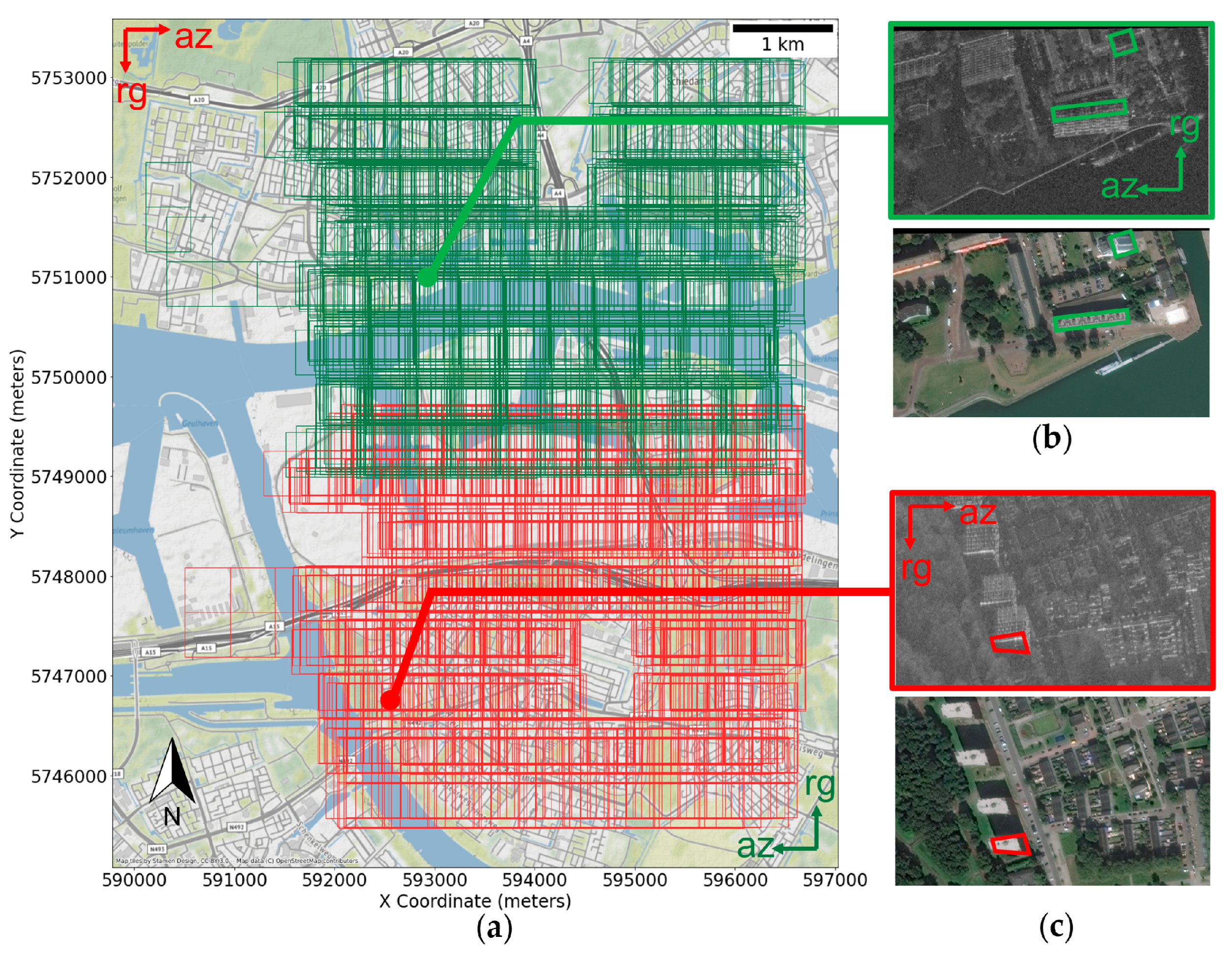
The SAR data has 2 orientations; both were captured using a north and a south facing sensor.
Figure 2a shows the tile over a base map of Rotterdam city, marking the position of images from orient1 (or north-facing) in green and orient0 (or south-facing) in red. The direction of flight is indicated by the azimuth (
az) arrow, while the direction where the sensor is facing is given by the range (
rg) arrow.
Each orientation creates different characteristics of how a building looks, namely the shadows and layover. The layover creates a projection of the building’s body onto the ground. It is caused by the side-looking nature of SAR imaging and the fact that SAR imaging maps pixel values based on the order of received echo. This is especially prominent in tall buildings.
The quad-channel SAR (also known as polarimetric SAR) is excellent for deep learning applications that benefit from the extra data. However, to showcase the effectiveness of data augmentation methods, we only used tiles from orient1 (covering the northern part of the city) and only a single channel HH polarization. This constraint enforces overfitting due to a limited data situation while still maintaining distinct land use cover of the port area and residential buildings. We chose only the HH polarization channel due to it being mostly available in SAR constellations such as GaoFen3, TerraSARX, and Sentinel 1 [
27].
2.2. Preparing the Dataset
The purpose of training a Deep Learning model is to predict well on new data, which the model never sees during training. This is called generalization. The proper way to develop a model is to prepare 3 separate datasets called the training set, the validation set, and the testing set. As their names suggest, each is used in a different phase of a model’s development. For each iteration of training, called an epoch, the model updates its weights by learning from the training set. At the end of each epoch, the model is tested on the validation set without updating its weights. This is used as a guideline for the Deep Learning practitioner to optimize the model or training parameters by studying the generalization ability over each epoch. Finally, when training is finished, the true performance of a model is determined by its score on a separate testing set.
To train our model, we used roughly half of the SpaceNet6 training set, which was constrained to a single sensor orientation and a single HH channel. We did not use a separate testing set. To evaluate the performance of our model and as a guideline for the impact of augmentation methods, we generated a validation dataset using the expanded version of SpaceNet6. This extra data was released later after the SpaceNet6 competition finished and consisted of unprocessed Single Look Complex (SLC) SAR data with additional polygon labels. We generated tile images from the SLC rasters with the same constraint as our training set: a single orientation and a single HH channel. We matched the exact preprocessing steps explained in [
9] using their provided Python library. The steps are:
Radiometric calibration using the Capella Space factor provided in each SLC raster’s metadata.
Converted the complex image into SAR-Intensity.
Performed multi-look to reduce speckle noise, using an average convolution operation with a 2 × 2 kernel.
Converted the pixel values to a log scale to create SAR Log-Intensity images.
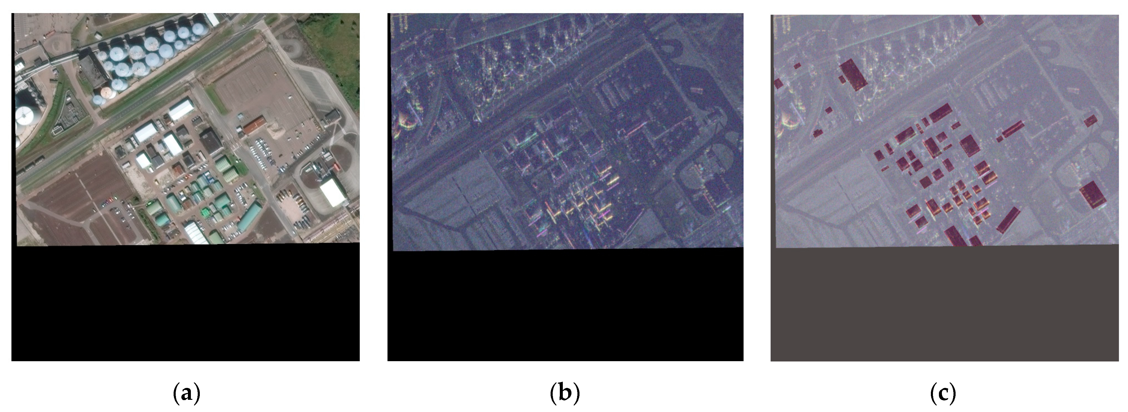
Orthorectified to correct geometric distortions caused by the Earth’s complex topography. Furthermore, resampled the raster to a spatial resolution of 0.5 m × 0.5 m per pixel. An example of a preprocessed SLC raster is shown in
Figure 3.
Generated non-overlapping tiles with a target resolution of 900 × 900 pixels within the boundaries of the testing set labels (outside the area in
Figure 2a) provided in the expanded dataset. We discard tiles with more than 40% of the no-data region.
We used a search algorithm to crop and remove the no-data regions. These are the black regions shown in the left and bottom parts of the image tile in
Figure 1. They were produced during the pre-processing stage of the dataset, stemming from the need to have a square non-overlapping tile image. The borders between the raster and the no-data regions created jagged lines due to slight affine rotation during orthorectification. Our experiments have shown these jagged lines to affect the results of pixel transformations, so in order to obtain consistent results, we have cropped them to a clean rectangle shape tile. The code we used in our methods is available as open source in
https://github.com/sandhi-artha/sn6_aug (last accessed on 9 April 2022).
2.3. Segmentation Model
Segmentation is the task of partitioning the image into regions based on the similarity (alike characteristic within the same class) and discontinuity (the border or edge between different classes) of pixel intensity. For building footprint extraction, there are only 2 classes: the positive examples, i.e., pixels belonging to a building’s region, and negative examples, which are the rest of the pixels (non-building). The deep learning model is given a pair of images and labels for training. The iterative process outputs a similar-sized image classifying each pixel as belonging to one of the two classes.
An encoder-decoder type architecture is commonly used for segmentation models, popularized by the famous UNet [
28] and its variations. For aerial imagery, DeepLab v3 [
29], PSPNet [
30], and Feature Pyramid Network (FPN) [
31] are commonly used. Based on a previous study [
32], we used the FPN architecture combined with the EfficientNet B4 backbone. EfficientNet is a family of CNN models generated using compound scaling to determine an optimal network size [
33]. For a deep learning model, the architecture refers to how each layer in the network is connected, while the backbone refers to the feature extraction part of the model.
Building footprints taken from overhead images have various sizes. To differentiate a building from the background, we need to see enough pixels representing the whole or most of the building. This means a higher spatial resolution is required for detecting buildings with a smaller area. A common method in computer vision to help the model learn these multi-sized objects is to use multi-scale input, i.e., the input image downscaled to different pixel resolutions. This is called an image pyramid (
Figure 4).
FPN uses feature pyramids instead. In the Encoder, the image input is scaled down using a dilated convolution operation which cuts the image dimension in half at each pyramid level. As the data flows up the pyramid, the top layer will have the least width and height (the original input’s size divided by 32) but the richest semantic information (1632 feature maps or channels). In a classification task, this is compressed further to output a vector with the same size as the number of classification labels [
31]. For a segmentation task, an output with the same spatial size as the input is required. Therefore, the top layer needs to be upscaled.
A 1 × 1 convolution filter is applied to the final layer in the encoder pyramid to reduce the number of feature maps to 256, without modifying the image dimension. As data flows down the Decoder’s pyramid, the width and height increase 2× using nearest neighbors upsampling. In the skip connections (yellow arrow), feature maps from the same pyramid level in the Encoder and Decoder were concatenated. A 1 × 1 convolution was used to scale the feature maps from the Encoder pyramid to 256. This provides context for better localization as the image gradually recovers in pixel resolution. Afterward, feature pyramids from the Decoder go through a Conv and Upsample operation (black arrow), resulting in modules with 128 feature maps and image dimension 1/4 of the original input. These are then stacked channel-wise, creating a module of 512 feature maps. A final Conv and Upsample operation reduces the number of channels to 1 and restores the image dimension back to the original input [
34].
2.4. Training Details
The training was performed in a Kaggle Kernel, a cloud computing environment equipped with a 2-core processor and an Nvidia P100 GPU with 16 GB of video memory (VRAM). The training pipeline was built using the TensorFlow framework. The Segmentation-Models library [
35] was used to combine the FPN architecture with the EfficientNet B4 backbone with no pre-trained weights. Adam [
36] was used as the optimizer with default parameters. We used a learning rate scheduler, which configures the learning rate
to gradually decay by a factor of
where
is the current epoch and
is the total number of epochs.
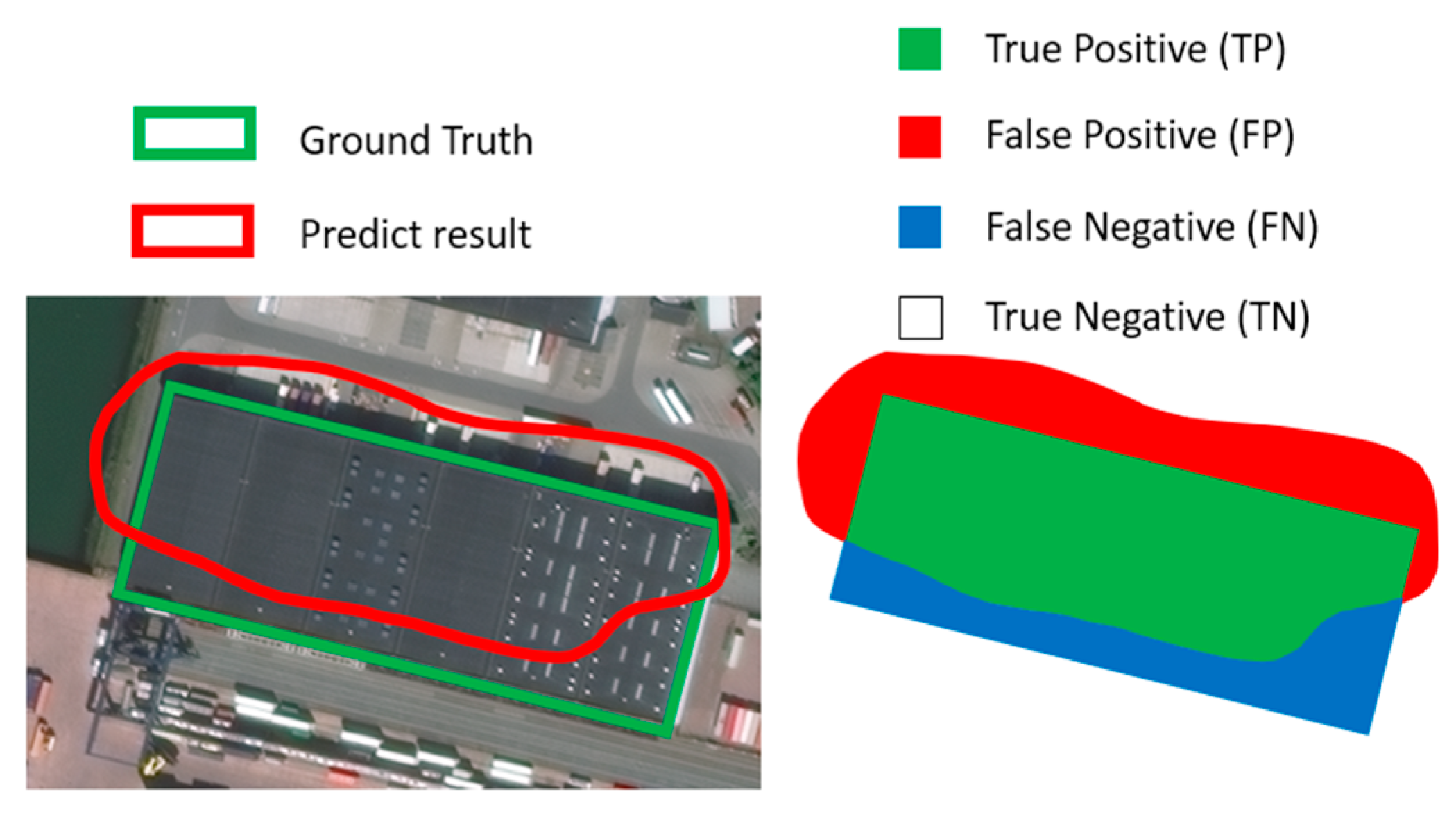
To evaluate the performance of our model, we use the Intersection over Union (IoU) as the metric. IoU is the ratio of overlapping between the predicted area and the real area (
Figure 5). In this case, it is a pixel-based metric. A higher IoU indicates a better predictive accuracy.
True Positives (TP) are pixels labeled as building and are correctly predicted as building. True Negatives (TN) are pixels labeled as background and are correctly predicted. False Negatives (FN) are misclassified background pixels, while False Positives (FP) are misclassified pixels of buildings.
Calculating statistics over each image tile in the training set, 20% of tiles have less than 1% positive samples (pixels classified as buildings) (
Figure 6a). This indicates that most tiles contain high negative samples (background pixels). One must be cautious in selecting a loss function for training a model on a skewed data distribution such as this because the negative samples will dominate the predictions. For example, using a binary cross-entropy as the loss function, the model will obtain a minor error even if it predicted the whole image as background pixels.
We experimented with several loss functions and concluded that Dice Loss leads to better convergence in this dataset. It is based on the Dice Coefficient, which is used to calculate the similarity between 2 samples based on the degree of overlapping. Dice loss is simply
. This results in a loss or error score ranging from 0 to 1, where 0 indicates a perfect and complete overlap.
2.5. Ablation Study
First, we studied the impact of each augmentation method in an ablation study, applying the same model and training configuration but applying different transformations to the dataset. To speed up this process, we trained and validated only a subset of our main training set. We divided it into 5 identical columned regions. The first and second columns were used as the mini-training dataset, while the last column was for the mini-validation dataset. We did not include the middle area in the mini training set to create a buffer (notice the high overlapping of tiles in
Figure 2a) which prevents data leakage between both sets. The mini-training set and the mini-validation set contain 37% and 23% images of the main training set, respectively. After concluding which augmentation works well for the mini dataset in the ablation study, we applied combinations of positively impactful transformations to the main dataset.
3. Data Augmentation
This section describes the data augmentations used in this study and how they were implemented during the model’s development. In general, the geometric transformations (including reduce transformation) were applied using TensorFlow operations, while pixel transformations were applied using the help of the Albumentation library [
37].
3.1. Types of Data Augmentation
3.1.1. Reduce Transformation
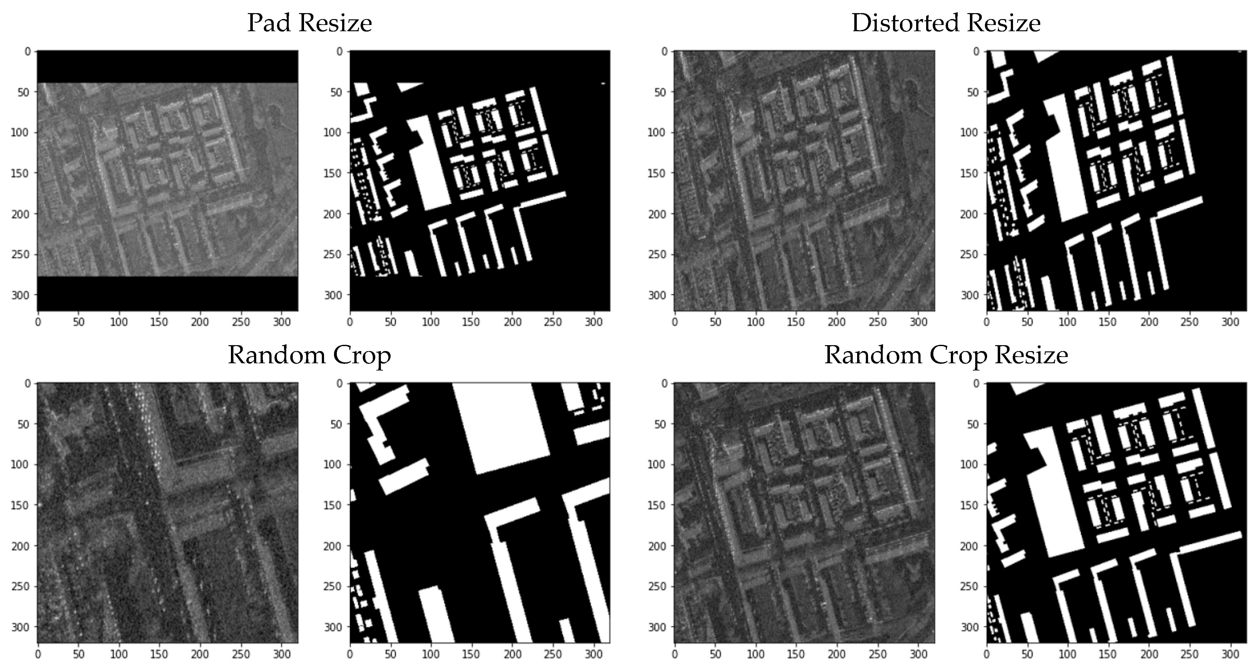
Cropping the no-data regions result in a varying aspect ratio for each tile that must be addressed. Square-shaped images are preferred as data input to simplify spatial compression and expansion of the image inside the model. The image size also needs to be reduced to fit into the GPU’s memory. We decided on the target resolution of 320 pixels by 320 pixels, which allowed the batch size of eight for the single P100 GPU. All resizing methods used the bilinear interpolation. Two main resize methods were tested:
Pad Resize: no-data regions are added back to create a square aspect ratio, taking the minimum pixel value of . This is similar to the original tile, but now the raster is centered with no jagged borders. Next, the image is downsampled to the target resolution.
Distorted Resize: rectangle shape tile is resized to the square target resolution, distorting the shape of the image, but no black regions are present.
This downsampling process can be exploited to introduce randomness that further increases the diversity of the training samples. Cropping at random locations gave better details than just resizing the whole image (
Figure 7). However, because it introduces randomness, these methods cannot be used as a reduction method for the validation dataset:
Random Crop: a random region with the size of 320 × 320 pixels is cropped out of the rectangle image. This preserves pixel scale since no downsampling is performed.
Random Crop and Resize: crops a random location with a random scaling, then downsample it to the target resolution.
3.1.2. Geometric Transformations
In computer vision tasks, geometric transformations are cheap and easy to implement. However, it is important to be aware of choosing the transformations’ magnitude that preserves the label in the image. For example, in optical character recognition, rotating a number by can result in a different label interpretation in the case of the numbers six and nine.
Flipping an image along the horizontal or vertical centerline is a common data augmentation method. Referring to
Figure 2a, the range direction
for this dataset is on the vertical or
y-axis, while the flight direction
is on the horizontal or
x-axis. The
Horizontal Flip does not alter the properties of a radar image. It would be as if the vehicle carrying the sensor was moving in the opposite direction. In contrast, the
Vertical Flip makes the shadows and layovers appear on the opposite side, creating inconsistency.
Rotation helps the model learn the invariant orientation of a building. We performed Rotation90 or quarter circle rotations and Fine Rotation with a randomized angle range, e.g., . Similar to Vertical Flip, the quarter circle rotation affects the imaging properties of the radar. The fine rotation exposes an area where image data are unknown. There are several ways to “fill” this blank area, and our experiments showed that leaving it to a dark pixel () gave the best result.
Shear is a distortion along a specific axis used to modify or correct perception angles (
Figure 8). Despite SAR being a side-looking imaging device, the processed SAR image appears flat owing to the orthorectification process that corrects geometric distortions. In
ShearX, the edges of the image that are parallel to the
x-axis stay the same, while the other two edges are displaced depending on the shear angle range.
ShearY is the exact opposite. We set the shear rotation to be randomized between an angle range of [−10°,10°].
Random Erasing is an augmentation method inspired by the drop-out regularization technique [
16]. It simply selects a random patch or region in the image and erases the pixels within that region. The goal is to increase robustness to occlusion by forcing the model to learn an alternative way of recognizing the covered objects. We have decided to fill the patch values with a dark pixel (
). The random erasing was implemented using CoarseDropout class from the Albumentation library. The region’s width and size were randomized from 30 pixels to 40 pixels, and the number of regions created was randomized from two to ten patches. The proposed geometric transformations are shown in
Figure 9.
3.1.3. Pixel Transformations
In airborne sensors, unknown perturbations of the sensor’s position relative to its expected trajectory can cause several defects such as radiometric distortions and image defocusing. To increase the model’s robustness when encountering these defects, we used noise injection methods. The common
Gaussian Noise was generated using the GaussNoise class, while
Speckle Noise was amplified by multiplying each pixel with random values using the MultiplicativeNoise class, both from the Albumentation library. Some images suffered from defocusing due to an unpredicted change in the flight trajectory, causing fluctuations in the microwave path length between the sensor and the scene [
38]. We simulate this defocusing by applying
Motion Blur with random kernel size using the MotionBlur class from Albumentation.
We used Sharpening with a high pass filter to improve edge detection. Consequently, this also increases other high-frequency components such as speckle.
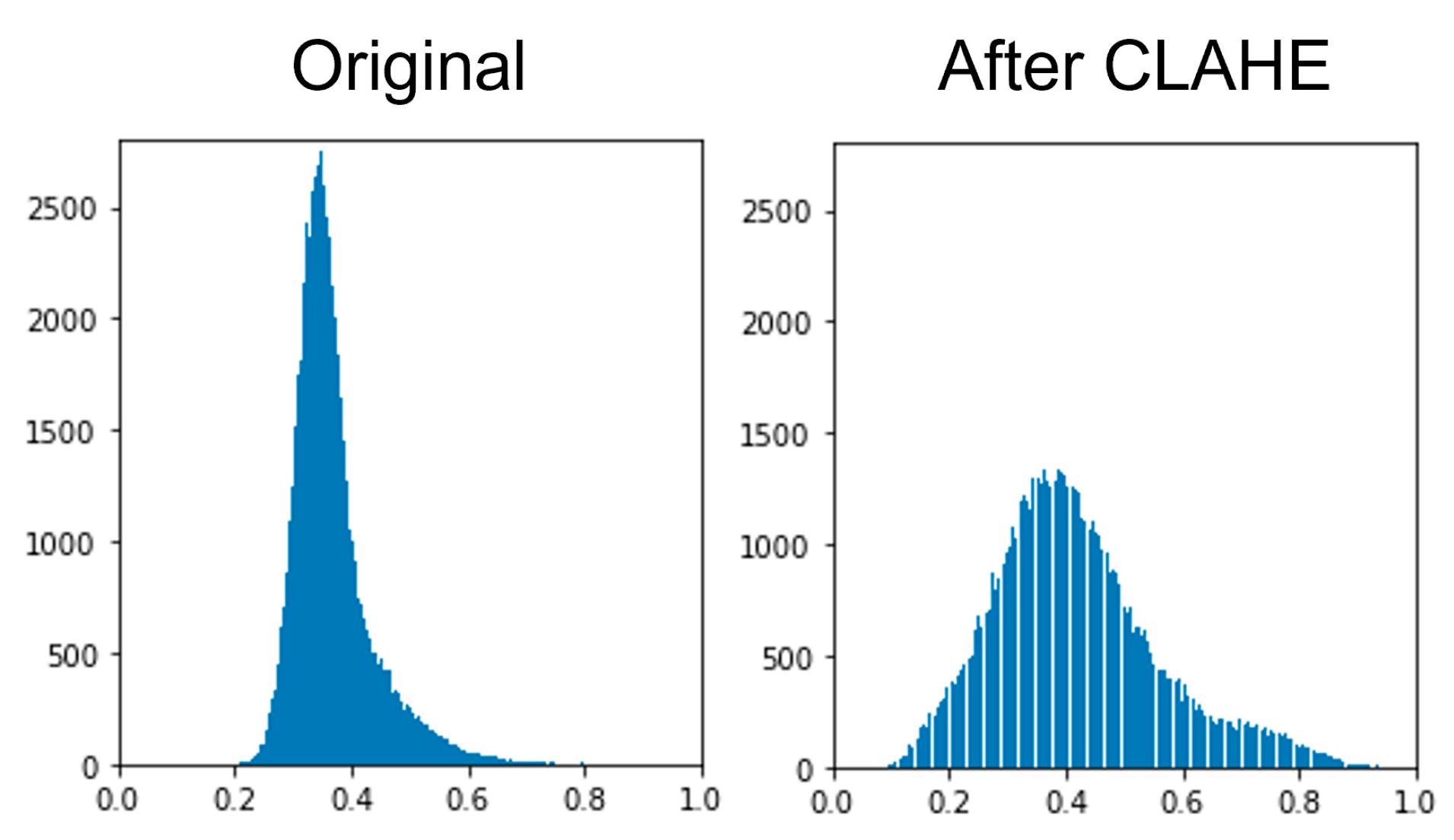
The SAR images in this dataset are SAR-Intensity in the log scale, also referred to as dB images. From samples of the dataset, we observed that the dB images have a pixel distribution close to Rayleigh and mostly populate a narrow area.
Figure 10 shows how histogram equalization methods stretch the pixel distribution to span the full range, increasing contrast and improving edge visibility. Contrast Limited Adaptive Histogram Equalization (
CLAHE) works best when there are large intensity variations in different parts of the image, limiting the contrast amplification to preserve details. We applied it using the CLAHE class from the Albumentation library. The proposed pixel transformations are shown in
Figure 11.
3.1.4. Speckle Filters
Although still categorized as Pixel Transformation, this subsubsection was created to provide more explanation for Speckle Filters. Similar to other coherent imaging methods (laser, ultrasound), SAR suffers from noise-like phenomena called speckle. This happens due to the interference of multiple scatterers within a resolution cell. Speckle takes form in granular variations of pixel values that can lower the interpretability of a SAR image for computer vision systems as well as human practitioners.
Speckle reduction filters such as a Box filter can smooth the speckle using a local averaging window. This is effective in homogenous areas, but in applications requiring high-frequency information such as edges, filters that can adapt to local texture can better preserve information in heterogeneous areas [
39]. A previous study [
32] has shown a slight performance gain by applying Low Pass filters with varying strength on the UNet model. In this research, we inspected the use of well-known adaptive speckle filters as a form of data augmentation, namely Enhanced Lee Filter (
eLee),
Frost Filter, and Gamma Maximum A Posteriori (
GMAP) Filter.
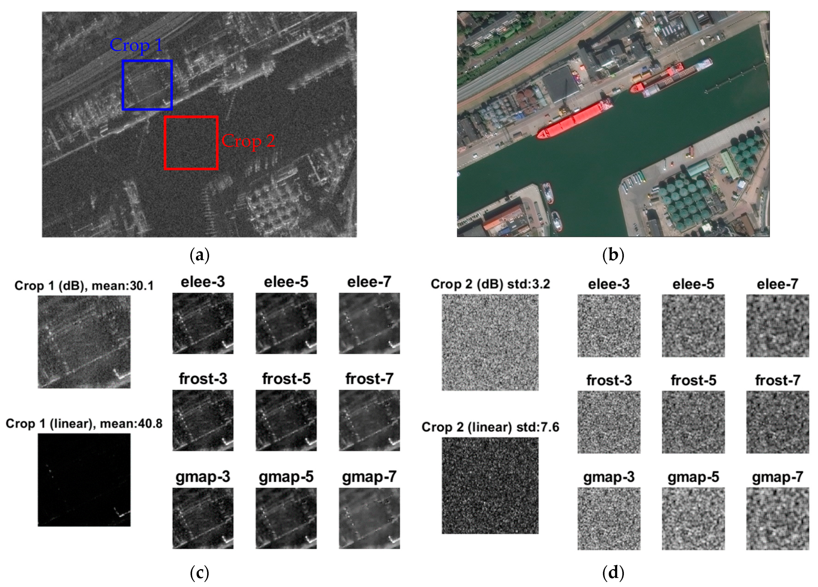
In
Figure 12a, two sample crops of size 150 × 150 pixels are shown for comparing filtration results. A good filter should retain the average mean of an image while reducing speckle [
40]. In homogenous areas, the standard deviation should ideally be 0. Speckle filters were applied in MATLAB to the SAR Intensity image (linear scale) and later converted back to the Log-Intensity image (dB scale). Results of filtering are shown in
Figure 12c,d, while the quantitative comparison is presented in
Table 1. We can observe that the GMAP filter was slightly better at preserving the average value and reducing variance in crops 1 and 2, respectively. The image’s Equivalent Number of Looks (ENL) also showed a reduction in speckle variance for all filters.
3.2. Data Augmentation Design and Strategy
We set a probability of 50% for an image to load either the original version or with data augmentations applied. The magnitude of the transformation was also randomized in a value range, increasing the variation in every iteration of training, except for flipping and quarter circle rotation, which had a limited set of transformations.
The order of transformations is important when multiple augmentations are combined during the main experiment. Pixel transformations are applied first to prevent the presence of no-data pixels from affecting the results. Following it is a reduced transformation, and finally, a geometrical transformation. When using multiple pixel transformations, it is important to combine them into a “One Of” group. By chance, only one of the transformations will be applied, preventing the creation of a disastrous result. In geometric transformation, there is no grouping, so an image has a chance to go through all transformations, which might increase no-data pixels but are generally less harmful than multiple filtering operations.
As categorized in [
10], there are three stages of applying Data Augmentation (DA): Online (on-the-fly), Offline, and Test Time Augmentation (TTA).
In Online DA, the input data is manipulated during training. This can lead to a bottleneck if a fast accelerator is used in training, but the augmentation algorithm is slow, leaving the accelerator mostly waiting for data. The advantage is that it does not store the inflated data in storage. On the other hand, Offline DA allows complex manipulation and will not bloat training time. However, since it is applied before training, it takes up storage, and the variations are pre-determined (less randomness). We used Offline DA only for speckle filtered images since they were processed outside the TensorFlow environment, and an image was stored for every applied filter. Other transformations in this study used Online DA, which can have a finer degree of randomness in every iteration.
In TTA,
additional images are generated from each test image
, where
is the number of augmentations applied during the inference or prediction stage. The model will then predict on
samples and the average sum will be taken as the final prediction. This method of predicting multiple transformed versions of the input mimics the theory of ensemble learning, where a group of models using different architectures or trained on different data combines their prediction to increase generalization. This was investigated in [
41], concluding that TTA helped reduce overconfident incorrect predictions compared to when using only a single model.
In a classification task, averaging predictions are straightforward since the output is an array with a size equal to the number of classes. In a segmentation task, one must be cautious to perform augmentations that modify the location of labels (in our dataset, the building footprints). If such methods are used, the solution is simply to revert back to the transformation before averaging the predictions.
4. Results
4.1. Ablation Study
In this isolated experiment, we measured the impact of each augmentation method. The model was trained on the mini-training dataset and evaluated on the mini-validation dataset. Results are shown in
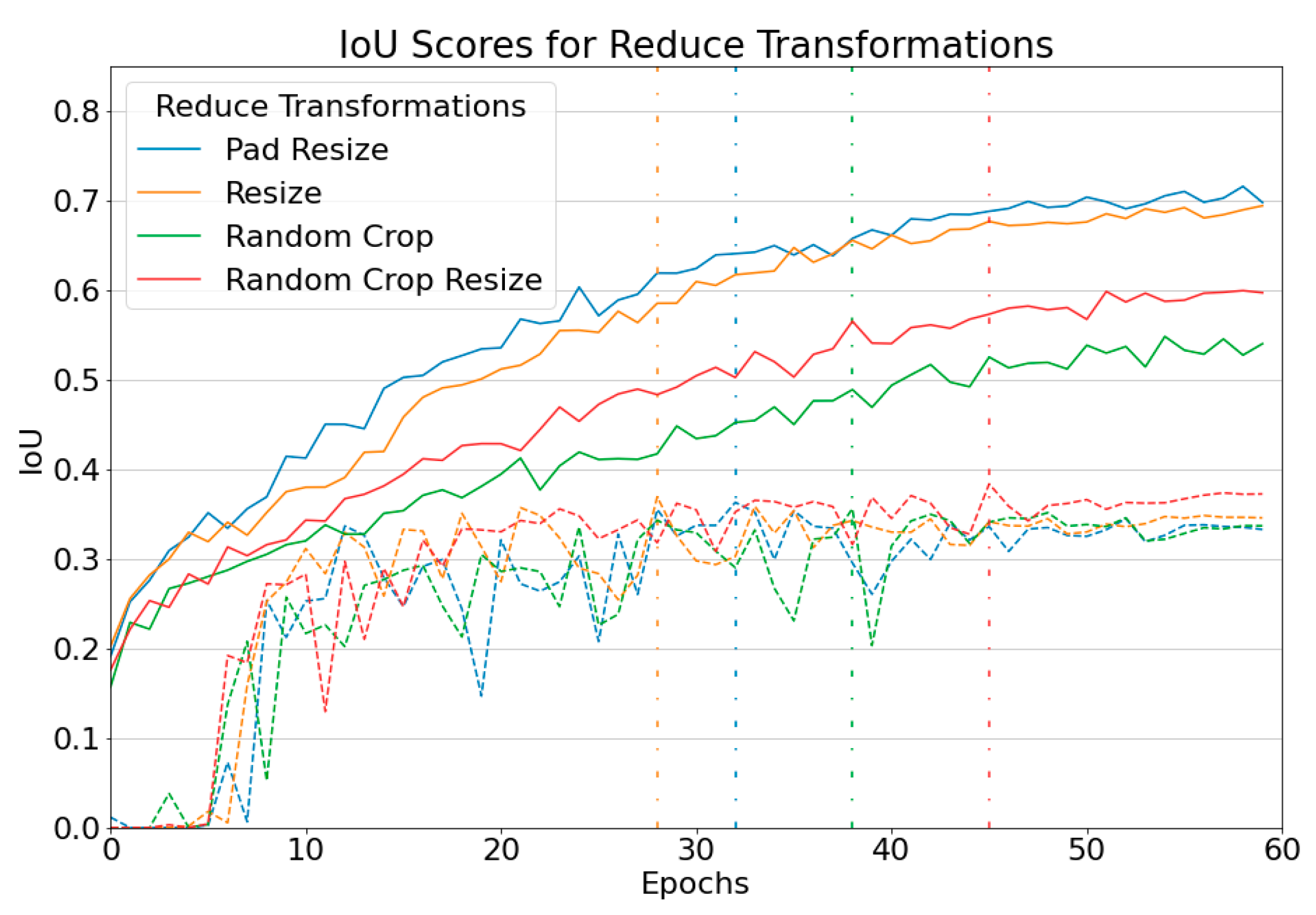
Table 2. Loss and IoU are the scores for the training set, while Val Loss and Val IoU are scores from the validation dataset. The training lasted for 60 epochs. The four metrics were taken at the best epoch, which is when the model obtained the highest Val IoU. We chose not to take the final score at epoch 60 to showcase the best performance of each augmentation objectively. The score at the last epoch was always worse than the best epoch because the training scores kept getting better while the validation scores stagnated or even deteriorated. This can be visualized in
Figure 13. The gap between both training and validation scores was less when an augmentation method was applied, which delayed overfitting, enabling the model to move into what is known as a Local Minima or a temporary performance peak.
To fit the image resolution to the model’s input, we used two basic Reduce methods: Pad Resize and Distorted Resize. A slightly better score obtained using Distorted Resize might indicate that the black paddings were distracting the model because the full scope of the raster’s space was not utilized. However, a problem arises when reshaping back the distorted prediction to the original aspect ratio, so we used Pad Resize as the Reduce method for the validation data. Adding randomness to the Reduce method using Random Crop Resize had the biggest performance gain compared to other augmentations. Randomizing the crop size gives the chance to see the image at different scales and details. Random Crop did not perform well due to the small static crop size of a 160 m × 160 m area, increasing the chance of encountering partial parts of a building.
Geometric transforms generally increased performance, except for Vertical Flip and Rotation90. Both were detrimental to the performance as they caused the extreme displacement of shadows and layovers’ location compared to the actual building footprint. Pixel transforms were not as effective, giving similar or slightly worse scores than the baseline. These augmentations affect the recognition of texture, an important feature when the edges of a building or its shape are unrecognizable due to occlusion or noise. However, this filtering can also be destructive as it also amplifies non-building patterns.
Training scores were generally lower when augmentations were applied, as the model struggles to find the underlying function among the additional variations. A strong increase in training scores for the GMAP speckle filter indicates better recognition of the training data. However, these variations were not shown among the validation data, hence the lower validation scores.
To validate the effects of our proposed data augmentation, we performed the Ablation Study on different mini datasets which we briefly described in the following:
- -
SAR Orient 0, which had the north facing sensor, opposite Orient 1 (see
Figure 2).
- -
PAN, also from the same SpaceNet6 dataset but uses the single band panchromatic images instead of SAR.
- -
Inria, a VHR optical RGB aerial imagery at 30 cm spatial resolution. To enforce the limited data configuration, we took only 15 images each from Austin and Chicago as the mini training dataset. As for the mini testing set, 10 images from Vienna were used. Each image was divided into 25 image tiles of 1000 × 1000 pixels. The RGB images were converted into grayscale for a fair comparison with the other single-channel mini datasets.
Figure 14 shows that performance gain and loss on the other datasets mostly agree with results in SAR orient1. Random Crop Resize, Horizontal Flip, and Fine rotation showed consistent gains over all datasets. Meanwhile, Rotation90 showed consistent dips in performance, which are more prominent in datasets from SpaceNet6. The result from PAN highlights the method’s impact on a similar geographic region (Rotterdam Port) but a different modality, while the result from Inria highlights the impact when exposed to the different urban settlements of multiple cities. However, due to the stochastic nature of deep neural networks, using an optimized model and training method fitted to one dataset might not translate to an optimal solution on another dataset, which has different distribution [
6]. Therefore, these directive insights should be further tweaked when working on a different dataset.
4.2. Main Experiment
Using similar concepts to those from the Ablation study, we experimented with several combinations of augmentation methods applied to the main training set and evaluated on our prepared validation set. The same model and training parameters were used except for the increased training duration to 90 epochs. This compensates for the additional variation and gives more room for the model to learn. A callback was set to monitor the best Val IoU score and labeled it as the best epoch. The following augmentation schemes were applied:
Baseline: No changes after applying a Reduce Transformation
Light Pixel: Motion Blur, Sharpen, and Additive Gaussian Noise
Light Geometry: Horizontal Flip, Fine Rotation , ShearY
Heavy Geometry: Horizontal Flip, Fine Rotation , ShearX , ShearY [−10,10], Random Erasing
Combination: Light Pixel + Light Geometry
Only Baseline used Pad Resize as the Reduce method, while the other combinations used Random Crop Resize. For every augmentation scheme, the model’s performance was taken at the best epoch and shown in
Table 3. Due to different datasets, the scores in
Table 2 should not be directly compared to results from this main experiment. The training time
was measured as the duration of training but shown in the table as a scaling factor compared to Baseline where
.
In line with results from the Ablation Study, geometric transformations had better scores than pixel transformations. Increasing the magnitude of transformation did not lead to an increase in performance, as shown by the lower scores obtained in Heavy Geometry. Increasing the diversity of transformations in Combination also did not improve performance despite consisting of transformations that showed positive impacts during the Ablation Study.
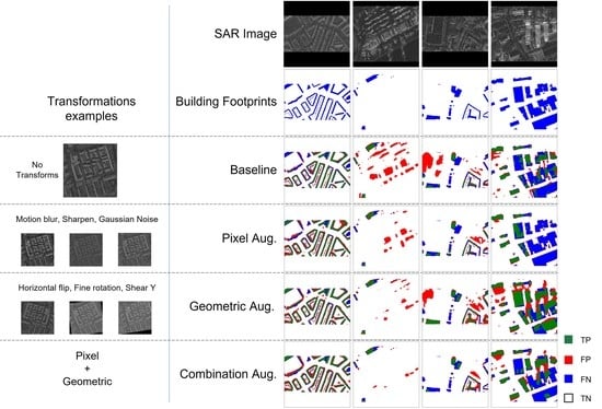
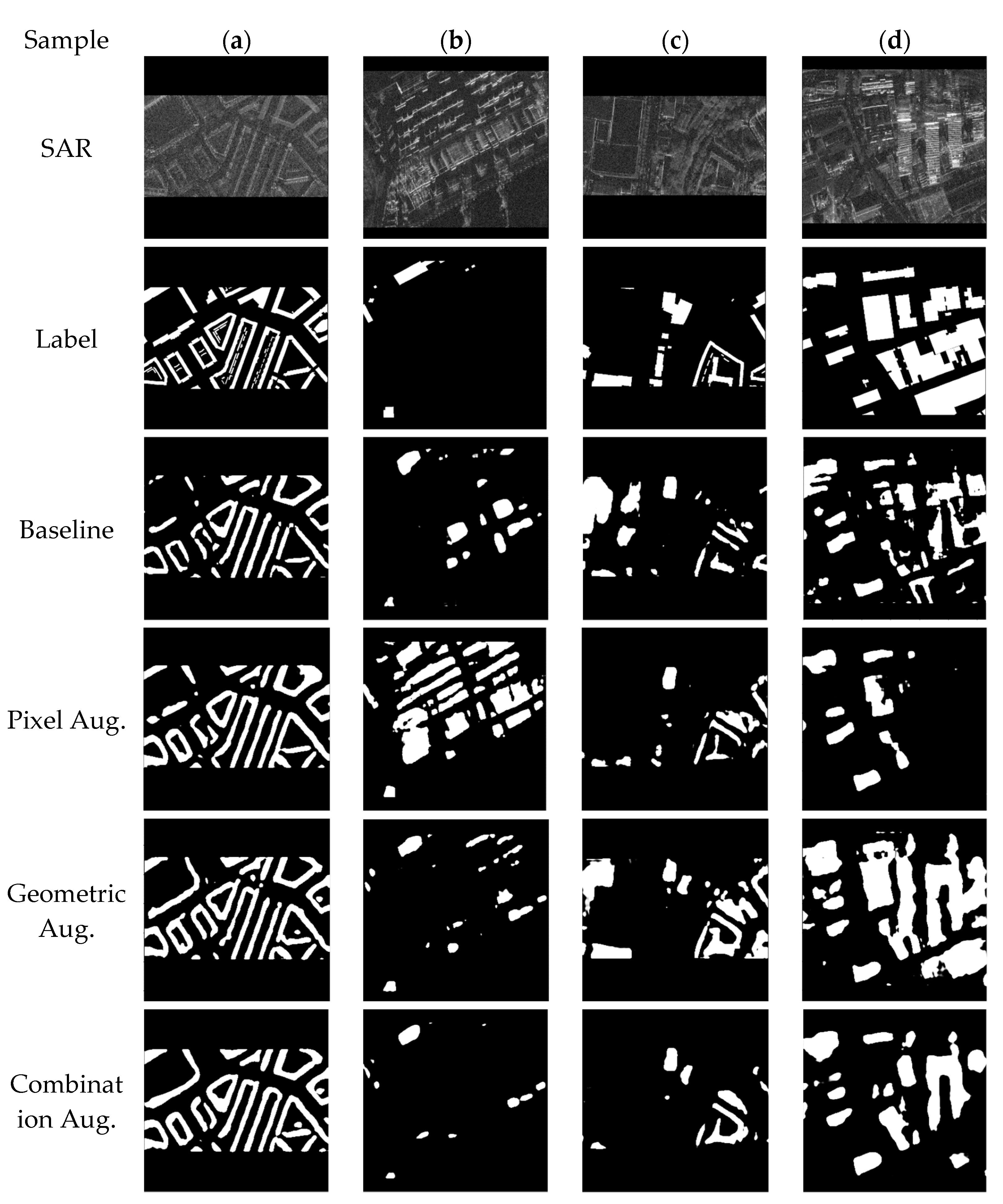
All models predicted well on medium height elongated residential buildings (
Figure 15a). Applying augmentation increases confidence, modeling a more accurate shape characterized by rooftop patterns. However, fine details of a building structure and small buildings remained undetected.
For an image tile of large negative samples (pixels belonging to non-building), pixel augmentations drive extra attention to high backscattering objects such as container storage and large shipping/port equipment made of metal (
Figure 15b). This leads to an increase in false positives. Geometric augmentations were less prone to this. However, Geometric augmentations overfit non-building objects with building-shaped backscatters, such as the fences surrounding a sports field (
Figure 15c). A combination of geometric and pixel augmentations seems to tune down these false positives and correctly recognize them as non-object patterns.
Occlusion was the biggest problem, especially related to high-rise buildings in dense areas (
Figure 15d). All models failed to recognize buildings occluded by the overlay of a neighboring high-rise building. Interestingly Geometric augmentations tend to classify the overlayed parts as positives.
Despite not using any augmentations in Baseline, the Light Pixel scheme, applied using the Albumentation library, managed to train slightly faster. This was caused by the callback function, saving the state of the model each time it sees a better-monitored value, requiring additional time on certain epochs. It shows that training duration is not an objective measurement due to the randomness involved. However, we still included it as a comparison. The other schemes show that adding more transformation methods will increase training time.
4.3. Test-Time Augmentation
The state of the models in the Main Experiment was saved at their best epoch, and TTA was applied after the training ended. We experimented with two methods for TTA:
TTA_1: Pad Resize was used for reducing image resolution. Transformations include Horizontal Flip, Rotate and ShearY . After predicting each sample variation, an inverse transformation was applied, and the average sum will be used as the final prediction. Total predictions per test sample: six.
TTA_2: The rectangle image tile was divided into two square patches with some overlapping in the middle. This slightly increased the detail by utilizing the whole image space and removing the black bars. Afterward, TTA_1 was performed on each tile. Finally, the two prediction patches were combined by averaging the pixel values in the overlapping region. Total predictions per test sample: twelve.
We applied TTA to the Baseline model and the best model from the Main Experiment, which was trained on the Light Geometry scheme. TTA comes at the cost of additional inference time
, which is a scaling factor compared to the Baseline’s inference time. It increases proportionally to the number of augmentations applied. Compared to the time required by re-training a model, the additional inference time to implement TTA was negligible. Results for TTA are shown in
Table 4.
The Baseline and Light Geometry model benefit from TTA_1, which consist of simple Geometric transformations. Interestingly, when TTA_2 was applied to the Baseline model, the performance was lower, as it predicted fewer positive samples from the two square patches. The Baseline model, trained on images with a fixed scale, had less confidence in predicting medium-sized buildings compared to the Light Geometry model, which had the chance to see variations of scaling thanks to the Random Crop Resize reduction method.
5. Discussion
Deep learning methods use vast parameter exploration. Results vary with different data, models, and training parameters (also known as hyperparameters). Our goal is to provide intuition based on our experiments of modifying the data while maintaining the model and hyperparameters unchanged. Radar images, including SAR, have unique properties that differ from optical images. Therefore, several transformations can result in poor performance. Selecting augmentation methods requires knowledge of the biases in the training data, either through statistical analysis, in the case of a large dataset, or through the manual inspection of samples. This helps reduce the search space instead of trying every available method.
Tiling is required in remote sensing images as it is impossible to fit a large raster directly to a model. The choice of target resolution will affect the detection of multi-scale objects, such as buildings. Introducing randomness by varying the scale and crop size during dataset loading is a cheap way of boosting performance since there is no need to store extra images, such as in the case of tiling with overlapping regions. However, cropping too much will increase the chance of a large object covering the whole space and hinder performance. No-data regions are inevitable when tiling a large raster, and in our experience, it is better to remove them before feeding the image tile to the model.
Our study shows that pixel transformations are not as effective as geometric transformations. The reason might be that kernel filters, which are the base of most pixel transformations, are already an integral component of the CNN model itself, thus, learnable by an adequately sized model.
Applying transformations at different stages of the model development has different tradeoffs. For instance, Offline DA can utilize the training images with their stored variations, all at once to train the model. We experimented on a dataset transformed with speckle filters and achieved similar scores to Random Crop Resize in
Table 2 but at the cost of 3.5× training time. This might be a good option when the data consist of only a few hundred samples and gathering extra data is unfeasible, such as in the case of classifying rare medical images.
We demonstrated that Test Time Augmentations (TTA) is a cheap method to boost test scores. However, applying a set of augmentations during the test did not achieve better scores when compared to applying the same set of augmentations during training. The model predicted the varying test samples better, had it seen these variations during training. Therefore, applying augmentations in both stages will result in better scores. When using Shear and Fine Rotation in TTA, the angle must be kept low because it removes some portion of the image (outside the image boundary) where it will not return when doing the inverse transformation after prediction. This is why quarter-circle rotations and flips are more commonly used as TTA because they retain the full image after inverse transformation.
6. Conclusions
This paper presents several data augmentation methods for semantic segmentation of building footprints in SAR imagery. By artificially increasing the training dataset, we improved the model’s generalization on unseen samples from the validation set, thereby reducing overfitting. The results show a 5% increase in Val IoU score when comparing the best augmentation scheme to the baseline model (no augmentation). Data augmentation can be very helpful in situations with limited data, either due to proprietary licenses or an expensive collection process.
For building detection in SAR, geometric transformations were more effective than pixel transformations. However, some transformations (such as vertical flip and quarter circle rotations) that alter key features of a building in SAR images were proven to be detrimental. Therefore, data augmentations must not be overused, especially since it takes more resources to train (either storage or processing time), which does not always lead to a better result. Test Time Augmentations showed an additional performance gain compared to augmentations applied only during training.
We hope this study can be used as a guide for future research to optimize object detection in a limited set of radar imagery or as an inspiration for investigating alternative methods to augment radar images. The search for effective data augmentation methods can be expensive; thus, automated approaches can save time and computing resources. These approaches have not yet been studied in this article. Furthermore, generating new data through generative models or the use of simulations remain interesting avenues to explore.


