PRISMA L1 and L2 Performances within the PRISCAV Project: The Pignola Test Site in Southern Italy

Abstract

In March 2019, the PRISMA (PRecursore IperSpettrale della Missione Applicativa) hyperspectral satellite was launched by the Italian Space Agency (ASI), and it is currently operational on a global basis. The mission includes the hyperspectral imager PRISMA working in the 400–2500 nm spectral range with 237 bands and a panchromatic (PAN) camera (400–750 nm). This paper presents an evaluation of the PRISMA top-of-atmosphere (TOA) L1 products using different in situ measurements acquired over a fragmented rural area in Southern Italy (Pignola) between October 2019 and July 2021. L1 radiance values were compared with the TOA radiances simulated with a radiative transfer code configured using measurements of the atmospheric profile and the surface spectral characteristics. The L2 reflectance products were also compared with the data obtained by using the ImACor code atmospheric correction tool. A preliminary assessment to identify PRISMA noise characteristics was also conducted. The results showed that: (i) the PRISMA performance, as measured at the Pignola site over different seasons, is characterized by relative mean absolute differences (RMAD) of about 5–7% up to 1800 nm, while a decrease in accuracy was observed in the SWIR; (ii) a coherent noise could be observed in all the analyzed images below the 630th scan line, with a frequency of about 0.3–0.4 cycles/pixel; (iii) the most recent version of the standard reflectance L2 product (i.e., Version 2.05) matched well the reflectance values obtained by using the ImACor atmospheric correction tool. All these preliminary results confirm that PRISMA imagery is suitable for an accurate retrieval of the bio-geochemical variables pertaining to a complex fragmented ecosystem such as that of the Southern Apennines. Further studies are needed to confirm and monitor PRISMA data performance on different land-cover areas and on the Radiometric Calibration Network (RadCalNet) targets.

1. Introduction

The PRecursore IperSpettrale della Missione Applicativa (PRISMA) mission, launched by the Italian Space Agency (ASI) at the end of March 2019, is a demonstrative spaceborne mission with the intent of developing new environmental products using the potential offered by the hyperspectral data. The mission [1] includes a hyperspectral imager covering the 400–2500 nm spectral range with 237 bands and a panchromatic (PAN) camera (400–750 nm). Currently, many countries, even though they are at different stages of development, are planning or are close to launching hyperspectral spaceborne sensors, such as the Environmental Mapping and Analysis Program (EnMAP) from DLR [2], the Surface Biology and Geology (SBG) from NASA–USGS [3,4], the Hyperspectral Imager Suite (HISUI) from Jaxa [5], the USA’s Earth Surface Mineral Dust Source Investigation (EMIT) [6], and the DLR Earth Sensing Imaging Spectrometer (DESIS) [7,8]. The PRISMA mission, being de facto the first new-generation European hyperspectral spaceborne mission, serves as a stepping stone for the further developments of the European spaceborne spectrometers (e.g., ESA CHIME [9], SHALOM [10], and ASI PRISMA-2 [10,11]) and the provision of new high-priority products focusing on different environmental themes. To retrieve quantitative information from PRISMA images, the key issue is the radiometric accuracy over the whole mission lifetime, as well as the availability of effective and consolidated procedures for the retrieval of accurate reflectance values in the Visible Near-InfraRed and Short-Wave (VNIR–SWIR) spectral range. These issues are crucial for the use of satellite hyperspectral data in physically based applications, aimed at the retrieval of bio-geophysical parameters and at accurate quantitative surface mapping [12,13,14]. This could contribute to improving the national and international capability to answer users’ needs [15] for different environmental and agricultural issues.

In this framework, ASI has supported a PRISMA calibration/validation (cal/val) program (the PRISCAV project [16]). The PRISCAV project aims to identify sites within Italian territory, possibly already equipped and involved in cal/val activities for other satellite missions, to be used as fiducial reference measurements. PRISCAV activities are performed with the knowledge that there are not calibration test sites in Italy and that sensor calibration activities could be performed only by using international calibration test sites such as those belonging to the RadCalNet network. Thanks to PRISCAV, many reference sites have been selected for different environmental scenarios pertaining to Italian territory, ranging from coastal to Alpine sites, to support the post-launch radiometric calibration and to guarantee the system and processing chain performances. Recently, three studies [17,18,19] have dealt with PRISMA performance analysis. The study by Cogliati et al. [17] was mainly based on a single PRISMA scenario. It evaluated the spectral, radiometric, and spatial performance and the entire data-processing operation of the Level 1 TOA radiance product acquired for a rural area in Italy and a highly textured area in the USA (the latter included for the geometric accuracy assessment). Conversely, in the research by Guanter et al. [18], the potential of different PRISMA images for the detection and quantification of methane point emissions from fossil fuel production activities was assessed in different oil and gas production basins in Algeria, Turkmenistan, the USA, and China. The study of Romaniello et al. [19] compared the performance of Hyperion, AVIRIS, and PRISMA for a dark target (reflectance lower than 0.05 from the VNIR to the SWIR) area ‘Piano delle Concazze’ (Mt. Etna, Italy). The results showed that PRISMA radiance had a mean bias of +5.22 Wm⁻² sr⁻¹ µm⁻¹ (about +20%) and +0.91 Wm⁻² sr⁻¹ µm⁻¹ (about +43%) with respect to MODTRAN simulations.

The present work refers to the activities performed to determine the performance of the PRISMA sensor in a mid-Apennines fragmented agricultural scenario, i.e., the Pignola test site. In the framework of the PRISCAV projects, the Pignola test site, within a typical Mediterranean landscape, was included among the selected Italian fiducial sites to enlarge the database of cal/val reference data for the continuous monitoring of PRISMA performance. The use of widespread reference sites in Italy is allowed by the PRISMA pointing capability of ± 20.7°, which permits six viewing opportunities for the same site within the revisit cycle of 29 days, thus allowing acquisition from different cal/val sites on a multitemporal basis.

With respect to the monitoring of the sensor’s radiometric performance, the Quality Assurance Framework for Earth Observation (QA4EO) project [20], developed in the context of the Group on Earth Observations (GEO, www.earthobservations.org; accessed on 18 December 2021), defines quality indicators (QI) to improve and evaluate the data quality of the imagery through standards and products. The Committee on Earth Observation Satellites (CEOS) Cal/Val also represents the main forum for the exchange of information and the sharing of good practices and cal/val protocols with the wider Earth Observation (EO) community. For the land product validation, the CEOS Land Product Validation (LPV) group [21,22] coordinates the validation activities for the quantitative assessment of EO products (biophysical variables).

The use of ground information from local test areas for spaceborne hyperspectral sensors such as PRISMA relies on the possibility of obtaining reflectance data that can be compared with other multispectral or hyperspectral payloads. An experiment on ground truth data collection contemporary to a Hyperion acquisition was conducted in 2015, within the joint ASI and Israeli Space Agency research project “Vicarious radiometric CALibration for orbital HYperspectral sensors” (V-CALHY) to test Hyperion performance for a restricted area. For this scope, Hyperion imagery was acquired on the same day (same orbit) for both the Amiaz site in Israel (31.07 lat., 35.36 long.) and the Maccarese test site in Central Italy. These images were used to independently derive Hyperion signal gain and offset. The results showed that the radiometric shift at the Amiaz reference sites were comparable to those acquired for the RadCalnet site [23]. The V-CALHY experiment at Amiaz showed a “percentage of difference” (PD) [24] (i.e., the normalized difference between the reference ASD soil spectral reflectance compared to Hyperion multiplied by 100) of about 5% in the VNIR, 650 nm; a value below 4% at about 1800 nm; and a PD between 5% and 9% in the far SWIR region (2200–2300 nm). These values were perfectly comparable with those derivable using more instrumented cal/val sites [24]. This experiment confirmed that rather small test areas could also be exploited for cal/val purposes of spaceborne hyperspectral data.

Based on the experience gained from these reference sites, the Pignola test site has been proposed to ASI as a solution to check and monitor the radiometric performance of PRISMA spectral radiances (L1 standard products) as well as the performance of the L2 reflectance standard product in the context of a typical fragmented agricultural site pertaining to Southern Apennine territory. The evaluation of PRISMA performance was achieved by comparing the L1 radiance with modeled L_TOA spectra. Simulations were obtained from the Modtran radiative transfer model for a Lambertian condition and by applying the atmospheric characteristics and the targets’ reflectance measured close in time to the PRISMA overpasses.

The PRISMA at-sensor radiance was compared to the modeled radiance obtained via radiative transfer models (RTMs) to assess the radiometric performance. The assumption for the chosen reference site relied on having accurate measurements of the ground reflectance target and the atmospheric characteristics, so that it was possible to accurately configure the applied RTM [23,25].

The contribution of this paper to the remote sensing community is to provide an evaluation of real PRISMA performance in terms of radiometric/reflectance accuracy based on suitable ground measurements and atmospheric profiles in a rural area of the Italian Southern Apennines, as depicted by root-mean-square error (RMSE), relative root-mean-square error (RRMSE), and relative mean absolute difference (RMAD) values measured from October 2019 to July 2021. Furthermore, a first assessment of the spatial pattern of coherent noise is presented.

The paper is organized as follows: in Section 2 (Materials and Methods) we first provide a brief description of the PRISMA hyperspectral payload [26] and of the ground measurements acquired on the Pignola site simultaneously with the PRISMA overpasses. Then, we describe the pre-processing applied to the ground measurements that were used later to configure the physical model before being used as a comparison with the L1 (Section 2.4.1) and L2 (Section 2.4.2) PRISMA images. Moreover, we present the image-based procedure applied to estimate the noise as well as the SNR. In Section 3, the radiometric and reflectance data, obtained, respectively, by MODTRAN simulations and an independent atmospheric correction procedure, are compared with the standard PRISMA L1 (Section 3.1) and L2 (Section 3.2) products, and the evaluation metrics are explained, while in Section 3.1, the noise retrieved from the L1 images is presented and discussed. Section 4 is devoted to conclusions.

2. Materials and Methods

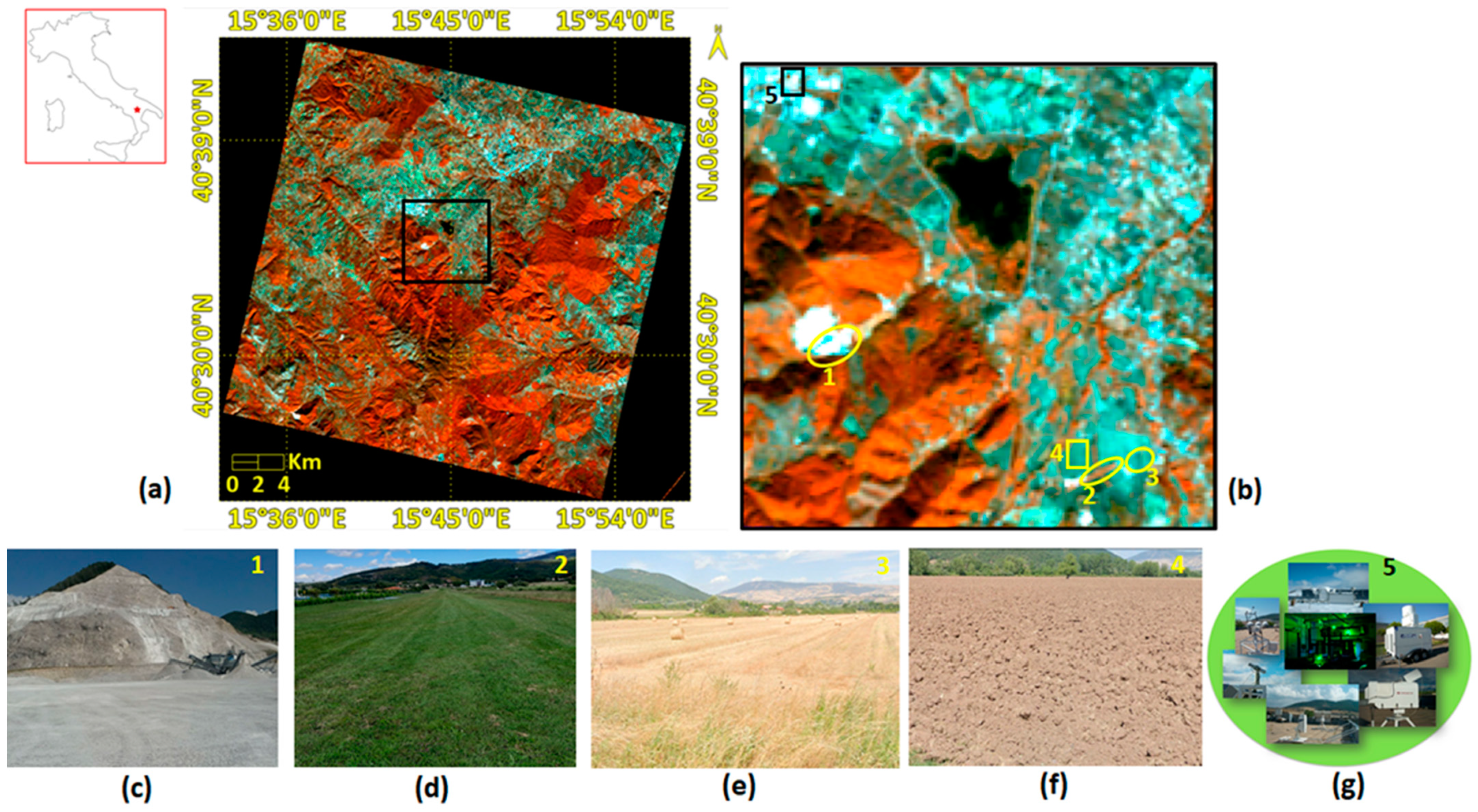
2.1. Study Area

Within the PRISCAV project [16], our activities pertaining to the validation of the PRISMA products were carried out on the experimental farm of Pignola (Italy), which belongs to the Lucanian Agency for Development and Innovation in Agriculture (ALSIA). This was mainly due to the opportunity to use both the experimental farm in Pignola (40.557303, 15.757921, 816 m a.s.l.) and the nearby CIAO (where CIAO stands for CNR-IMAA Atmospheric Observatory: CNR—Consiglio Nazionale delle Ricerche; IMAA—Istituto di Metodologie per l’Analisi Ambientale; http://www.ciao.imaa.cnr.it/; accessed on 10 December 2021), part of the ACTRIS (Aerosol Clouds Trace Gases Research Infrastructure; https://www.actris.eu; accessed on 5 December 2021). The Pignola experimental farm extends over 140 hectares, mostly consisting of arable land, pastures, and coppice with tall trees (Figure 1). The farm has a cereal–forage specialization and hosts a fully equipped agrometeorological station. The Pignola site is part of the regional agrometeorological network, consisting of thirty-eight agrometeorological stations, organized within the Lucanian Agrometeorological Service (SAL) (http://www.alsia.it/opencms/opencms/Servizio/SAL; accessed on 1 December 2021). Apart from the arable surface provided by the farm, within the PRISMA swath centered in Pignola, other reference surfaces are available for comparing simulated TOA with respect to that measured by PRISMA.

2.2. PRISMA Dataset

The “PRecursore IperSpettrale della Missione Applicativa” (PRISMA) stems from the previous ASI investments in the field of hyperspectral payloads (e.g., the Hypseo and JHM missions) and in satellite platforms (e.g., MITA/PRIMA), from which ASI acquired competency in the development and execution of optical missions and EO products. PRISMA is an Italian technological demonstrative and preoperational hyperspectral mission launched in March 2019.

The PRISMA mission combines two payloads, a hyperspectral prism spectrometer and a panchromatic camera. A complete technical description is given in [26], including the pre- and in-flight radiometric calibration procedures. The hyperspectral payload has a push-broom design providing hyperspectral imagery (237 bands) at a ground sampling distance (GSD) of 30 m over a swath of 30 km (

Table 1. PRISMA payloads’ main characteristics. The first column reports the requirements, while the last three specify the sensor performance as derived by the Leonardo Company and reported by [17].

	Requirements	VNIR	SWIR	PAN
Spectral range	400–2500 nm	400–1010 nm	920–2500 nm	400–700 nm
Spectral resolution (FWHM)	<15 nm	9–13 nm	9–14.5 nm	-
Spectral bands		66	171	1
SNR	≥160–200 (400–450 nm) ≥200 (450–1000 nm) ≥200 (1000–1750 nm) ≥100 (1950–2350 nm) ≥100 (PAN)	161–209 (400–450 nm) 200–450 (450–1000 nm)	380–800 (1000–1300 nm) 200–400 (1500–1750 nm) 100–200 (1950–2350 nm)	191
Absolute radiometric accuracy	≤5%	≤5%	≤5%	≤5%
Swath width		30 Km; 2.77°
Ground sampling distance (GSD)		30 m	30 m	5 m
Orbital altitude		620 Km

). The use of a prism as a dispersing element causes a nonuniform bandwidth along the VNIR and SWIR focal plane array. The bandwidth and the center wavelength (CW) are not constant for each acquisition, as they depend on the optical bench and instrument temperature. These changes are provided in matrix format within the PRISMA native Level 1 product HDF-EOS5 format, for both the VNIR and the SWIR, containing the center wavelength (CW) and FWHM pertaining to each acquisition. For the scope of this study, L1 TOA radiance units and L2C ground reflectance were applied. A more precise description of the processing is available in the PRISMA Products Specification Document (ASI, PRISMA Products Specification Document, Issue 2.1, accessed on 14 January 2022).

Over the Pignola site, different PRISMA acquisitions were planned.

Table 2. PRISMA acquisitions for the Pignola test site (Italy).

Date	Cloud Coverage (%)	View Zenith Angle (°)	Solar Zenith Angle	AeronetAOD@550 nm	Atmospheric Measurements	Ground-Based Measurements	Contemporary S-2 Data
14 October 2019	0.31	−4.14	49.90	0.09	√	√	n.a.
15 January 2020	0.58	2.31	22.45	0.05	√		√
1 July 2020	0.07	−3.91	22.34	n.a.	√	√	√
17 August 2020	2.55	14.35	30.00	0.21	√	√	√
23 November 2020	4.60	−3.71	62.08	0.02	√	√	√
22 December 2020	2.41	−3.9	65.57	0.02	√	√	n.a.
1 July 2021	0.04	−16.15	23.67	n.a.	√	√	√

lists the images employed for this paper. Moreover, most of the PRISMA imagery was acquired on the same date as the optical Sentinel-2 (S-2) imagery. As additional surfaces, wide enough to be visible at the PRISMA spatial resolution, we also selected as fiducial reference measurements: (a) a limestone quarry representing a highly reflective target with peculiar spectral behavior related to limestone and dolomite; (b) an airfield strip; (c) a wide shed with white plastic coverage that had specific absorption features in the VNIR and SWIR spectral regions.

2.3. Ground Measurements

Simultaneously with the PRISMA acquisitions, ground-based optical measurements and atmospheric characterization (from the CIAO, close to the study area) were gathered between 2019 and 2020 at the Pignola farm test site. Atmospheric properties and field surface reflectance measurements were applied to configure the parameters of the radiative transfer models and then to simulate TOA radiances to be compared to those acquired by PRISMA.

2.3.1. Field Spectroscopy Measurements

Ground reflectance and radiance measurements were collected in the test area to capture the spectral variability of the main surface material characterizing the area according to the season. The spectral measurements were collected with a FOV of 25° at a height of 1 m above soil across the 350–2500 nm spectral range, using the Analytical Spectral Device (FieldSpecPro, #6255 and FieldSpec4 #18936) FieldSpec (ASD Inc., Denver, Boulder, CO, USA), with a spectral resolution of 3 nm in the VIS–NIR range (350–1050 nm) and of 10 nm in the SWIR range (1050–2500 nm). With the ASD spectro-radiometer, configured to an average of 20 readings for each measurement, we sampled five transects within a 60 × 60 m Elementary Sampling Unit (ESU), according to the scheme of Figure 2, during stable sky conditions. In the field, reference points within each ESU were drawn with the help of ranging rods positioned with GPS. Data collected along the five transects were then averaged.

Moreover, at the same time as PRISMA acquisitions, irradiance measurements were collected from a Spectralon panel at a viewing angle of 45°. Target spectral reflectances were obtained by combining radiance and irradiance data using the ASD processing software (View Spec Pro 6.0.; ASD Inc., Denver, Boulder, CO, USA). ESU reflectance data were further aggregated and averaged to incorporate the whole range of the ESU variability. The ESU sampling strategies were applied to each target of interest: (a) bare soil, (b) non-photosynthetic vegetation as wheat residues, (c) photosynthetic vegetation as green meadow corresponding to an airfield, and (d) limestone surface pertaining to an active quarry, in accordance with the results of the Amiaz experiment that highlighted a good performance when using targets of limited extension.

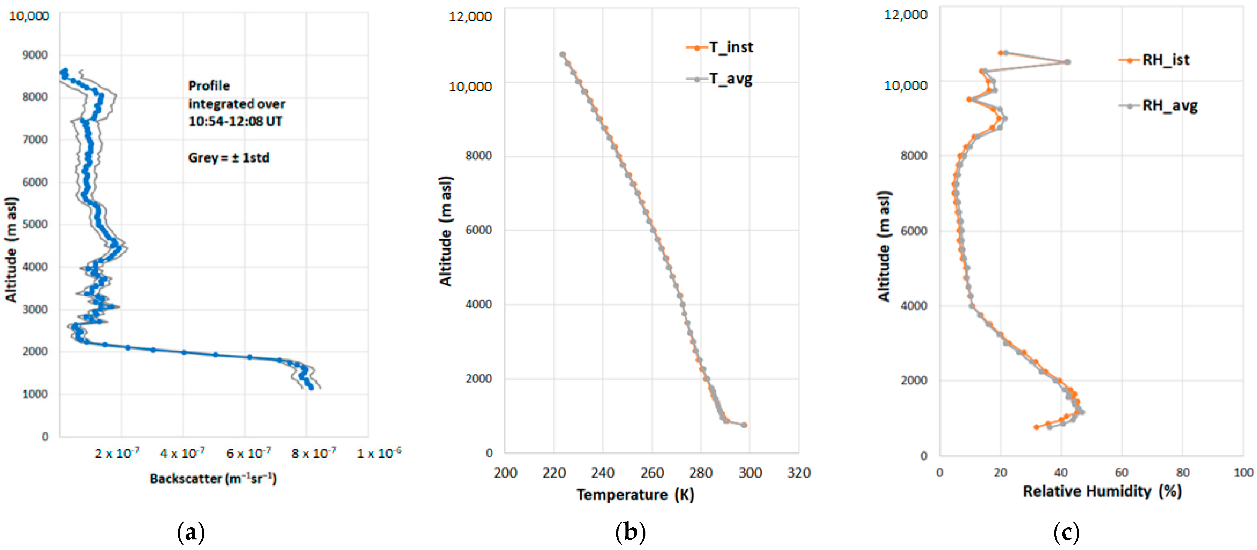
2.3.2. Ground-Based Atmospheric Measurements

Atmospheric characterizations over the test area during PRISMA acquisitions were provided by the CIAO [27], which is one of the most advanced infrastructures for ground-based remote sensing in Europe, equipped with multiwavelength lidar and scanning cloud radar [27]. The CIAO consists of a combination of advanced systems able to provide high-quality long-term observations of aerosol and cloud properties. It is equipped with the reference lidar systems for the ACTRIS component. The CIAO’s geographic position, within the Mediterranean basin but in a mountainous area, and far from big cities, makes the observatory a perfect location for investigating different aerosol types and atmospheric processes and setting up experiments with the support of the researchers and technicians operating the observatory.

For the aims of the present work, the following instruments were used:

• Multiwavelength Raman and depolarization aerosol lidar working at 355, 532, and 1064 nm, providing vertical profiles of the backscatter (at 355, 532, and 1064 nm) and particle depolarization ratio at 532 nm, and, in night-time conditions, the aerosol extinction (355 and 532 nm).
• Raman and depolarization aerosol lidar at 355 nm, providing vertical profiles of the aerosol extinction (in night-time conditions), backscatter, and particle depolarization ratio at 355 nm. Since it is remote-controlled, this system was used as a backup solution when the operation of the multiwavelength Raman lidar was not possible due to restrictions imposed during the COVID-19 pandemic.
• Autonomously operating sun photometer, part of the AERONET network. In daytime conditions, it provides cloud-screened, columnar aerosol optical depth at different wavelengths in the UV–near-IR spectral range.
• Microwave radiometer profiler, which measures the sky brightness temperature (Tb) at 12 frequencies, providing 24 h profiles of temperature and relative humidity.

Aerosol lidar measurements were available for the observational days listed in Table 2, except for 1 July 2020, when instrumental problems inhibited the measurements. The multiwavelength system was always used, except for 17 August, when the automatic 355-only system was used. Observations from the photometer were available for all the dates, except for 23 November, when the system was undergoing calibration procedures. Cloud-screened data were available in version 2 of the algorithm for all the dates.

2.4. PRISMA Data Analysis

This section describes the work carried out to assess the PRISMA behavior in terms of (a) radiometric evaluation when compared to the field measures, (b) cross-validation with respect to S-2 images when acquired simultaneously, and (c) signal-to-noise ratio (SNR) and images residual artifact assessment.

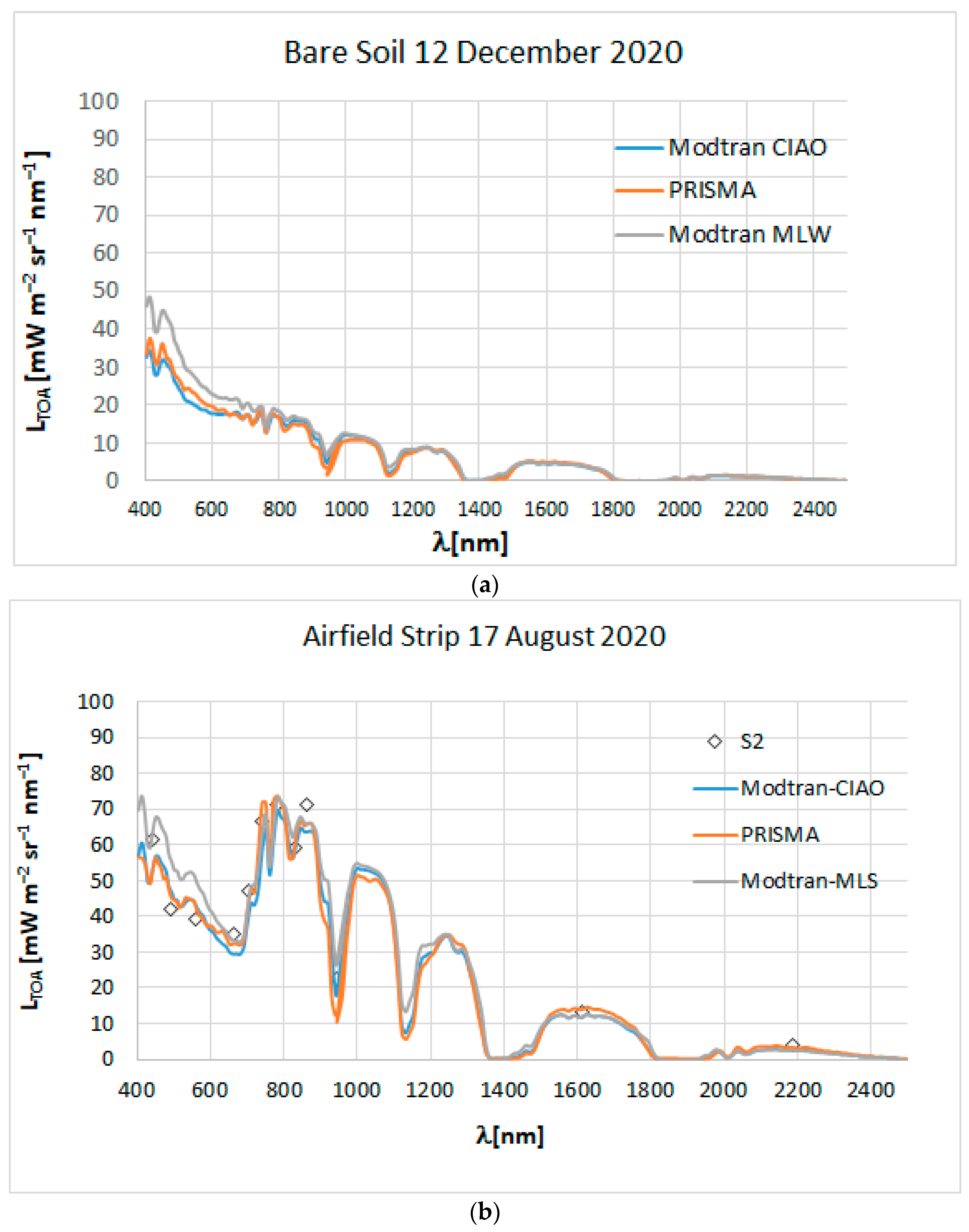
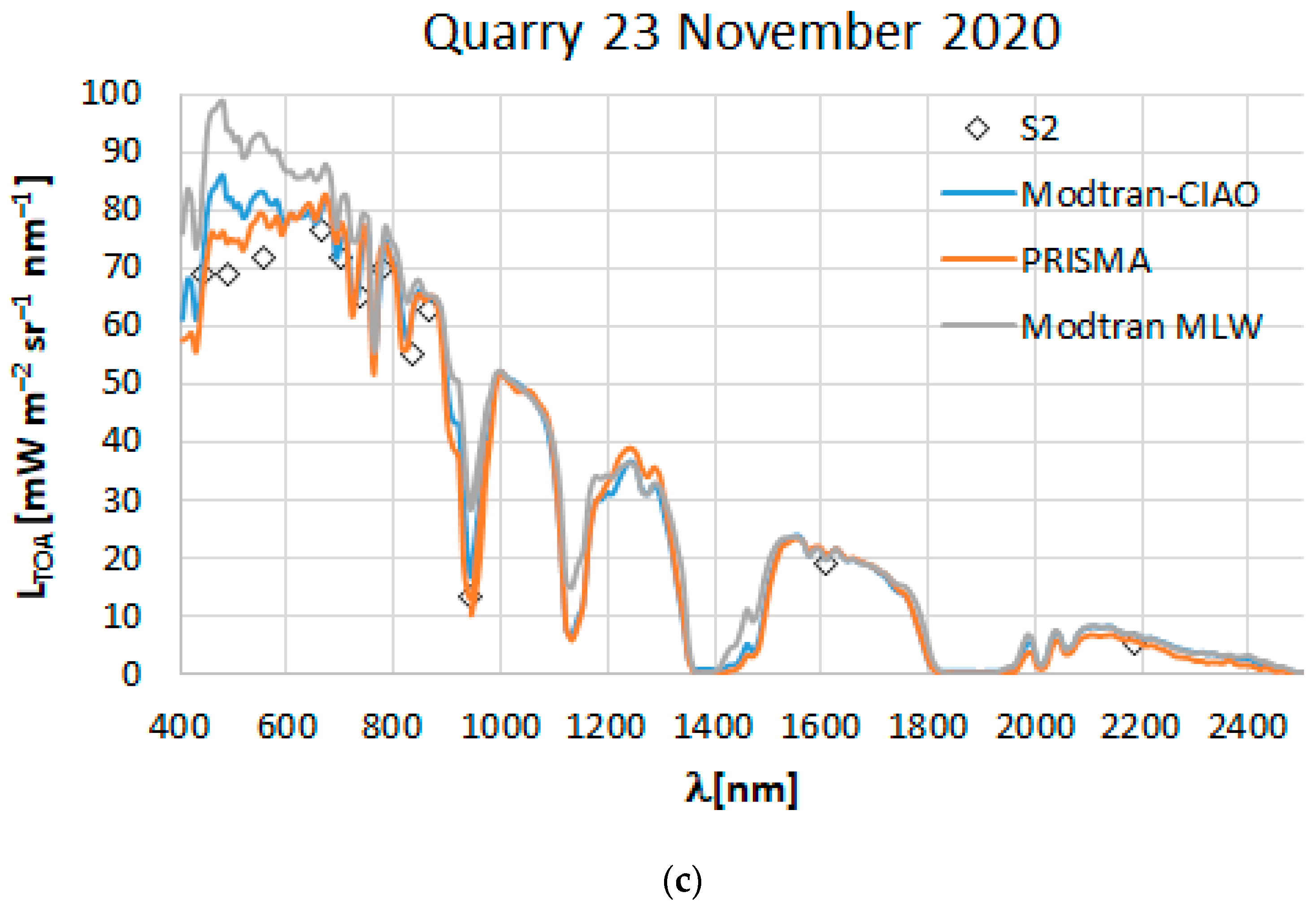
2.4.1. PRISMA Radiances: L1 Product Evaluation

The MODTRAN4 [28] radiative transfer code was used to simulate the PRISMA L_TOA starting from the in situ atmospheric characterization and land reflectances. The MODTRAN-derived L_TOA radiance in the direction of the sensor can be described as the sum of three terms, in the order in which they appear in Equation (1): (a) the reflected radiance from the surface (target radiance); (b) the atmospherically scattered direct solar radiation (path radiance); and (c) the diffuse upwelling flux scattered into the direction of the sensor (adjacency effect). The TOA calculation applied corresponds to the following formula:

$$L_{TOA}={\tau }_v\times E_d\times R_{rs}+L_{*}+L_a$$

(1)

where, τ_v is the upward atmospheric transmittance, E_d the total radiance at the surface, R_rs the surface reflectance, L_* the path radiance, and L_a the environmental effect. In our case, R_rs was measured by an ASD spectrometer in the field at the time of PRISMA image acquisition. Concisely, the L_TOA radiances were simulated assuming a uniform Lambertian surface and horizontally homogeneous atmospheric layers stratified according to the CIAO profiles in cloudless conditions. The environmental effects were calculated according to [29] by using MODTRAN simulations, setting the maximum visibility and alternately setting the surface reflectance to that of a blackbody and to a reference reflectance pertinent to the average reflectance around the target. Therefore, the contribution of the environmental reflectance was assessed by a point-spread function according to [25,29].

Each MODTRAN run, used to calculate the L_TOA, was configured with the aerosol optical thickness, the column water vapor (RH), and T vertical atmospheric profiles using 33 layers derived from the CIAO soundings (Figure 3).

During PRISMA acquisition dates, the CIAO measured the backscattering profiles at 532 nm (in one case, only the profile at 355 nm was available). The backscattering profiles were then converted into backscattering values at 550 nm. Moreover, as the backscattering measured in units of m⁻¹ sr⁻¹ was not usable in the MODTRAN RT code, which accepted only the extinction coefficient measured at 550 nm for the aerosol profile configuration, the aerosol backscatter at 355 nm (measured by the CIAO) was converted into aerosol extinction. A fixed extinction-to-backscatter ratio of 55 sr (based on climatological values recorded at the CIAO) was considered, so that:

$$Ext=Bck\ast 55sr$$

(2)

The extinction-to-backscatter ratio depends on the microphysical properties of the aerosols (such as refractive index, dimension, and chemical composition) [30]. However, aerosol typing studies and 20 years of systematic measurements [31,32] allow the conversion of backscatter into extinction, reducing the uncertainty in the derived value of extinction due to the lidar ratio assumption to the range of about 15%.

Then, the extrapolation from 532 nm (and 355 nm when needed) to 550 nm was carried out assuming an Ångström exponent (AE) of 1, as derived by the climatological values recorded at the CIAO. Due to the small difference in wavelength, the uncertainty in the extinction profile at 550 nm due to a variation in the AE of 0.5 was below 2%. Therefore, the extinction coefficient (Ext) was derived according to the following formula:

$${Ext}_{550}={Ext}_{532}{\left(\frac{532}{550}\right)}^{AE}$$

(3)

Considering the agricultural context of the area, a rural aerosol model was selected for all the simulations. Each MODTRAN run was configured with the proper line of sight based on the solar zenith and azimuth angles at the time of the satellite acquisition and by imposing the actual PRISMA viewing zenith angle. RT calculations were obtained in high resolution in the 400–2500 nm spectral range using a 1 cm⁻¹ resolution and selecting DISORT multiple scattering with 8 streams and the common Kurucz solar irradiance model. The Kurucz model was selected as it is widely applied and because the authors of [30] estimated the difference in the total integrated solar irradiance derived by different commonly used models as being less than 1%. A summary of the RT configuration parameters used is listed in

Table 3. List of the configuration parameters used for the RT L_TOA simulations.

Parameter	Unit	Values
Spectral range	nm	400–2500
Solar irradiance		Kurucz
Molecular band model resolution	cm−1	1
DISORT number of streams		8
Pressure profile	mb	CIAO according to date
Temperature profile	K°	CIAO according to date
Water vapour profile	RH	CIAO according to date
Aerosol model		Rural
Extinction @550 nm	Km−1	CIAO according to date
Surface height	km	0.750
SZA	deg	According to date
SAA	deg	According to date
VZA	deg	According to date
True surface albedos		According to ASD (Lambertian condition)

.

The MODTRAN input and output tapes were generated and processed with an ad hoc IDL code that allowed the extraction of the parameters used to simulate the L_TOA according to Equation (1). RT simulated L_TOA values were finally convolved to the real PRISMA spectral response function assuming a Gaussian shape function [17,18]. Response functions were modeled for each PRISMA image using the center wavelength (CW) and the full-width at half-maximum (FWHM) as retrieved from the ancillary data. The CW and FHWM, pertaining to each PRISMA acquisition, were extracted directly from the L1 HDF-EOS5 PRISMA file.

Radiometric consistencies were determined by the direct comparison of the MODTRAN simulated L_TOA, using the ESU spectral information (radiance on a white Spectralon panel) collected in situ by an ASD field spectroradiometer contemporary to PRISMA acquisitions, with the PRISMA real radiances.

PRISMA radiometric consistency was assessed by computing accuracy metrics to describe the degree of significance of the simulated radiance values with respect to the observed PRISMA radiance values. The applied metrics were mainly those described in [33], which are usually applied to evaluate a model’s prediction performance. As reported in

Table 4. Performance metrics applied for this study, where $y_i$ is the observed variables, $\overline{y}$ is the mean of the observed variables, ${\widehat{y}}_i$ is the estimated variables, n is the number of bands, and m is the number of images.

Name	Equation
Coefficient of determination (R2)	$R^2=1-\frac{{{\displaystyle \sum }}_{i=1}^n {\left(\widehat{y_i}-y_i \right)}^2}{{{\displaystyle \sum }}_{i=1}^n {\left(y_i-\overline{y} \right)}^2}$
Relative bias	$rBias=\frac{{{\displaystyle \sum }}_{i=1}^n\left(y_i-{\widehat{y}}_i\right)}{{{\displaystyle \sum }}_{i=1}^{n}y}\times 100$
Root-mean-square error	$RMSE=\sqrt{\frac{{{\displaystyle \sum }}_{i=1}^n{\left(y_i-{\widehat{y}}_i\right)}^2}{n}}$
Relative RMSE	$RRMSE=100\times \frac{RMSE}{\overline{y}}$
Relative mean absolute difference	$RMAD=\frac{{{\displaystyle \sum }}_{i=1}^m\left|y_i-{\widehat{y}}_i\right|}{{{\displaystyle \sum }}_{i=1}^m{y}_i}\times 100$

, they were: (a) the coefficient of determination (R²); (b) the root-mean-square error (RMSE); (c) the relative RMSE (RRMSE); and (d) the relative bias (RBIAS), which indicates the relative estimation errors between simulated and real PRISMA spectra. RBIAS together with R² provides a deviation between the observed and simulated radiance, (e) the relative mean absolute difference (RMAD). The R² metric measures the percent of the variance of the PRISMA real data that the predicted radiance data can explain and is the common metric applied to express the goodness of fit of the model in terms of the linear correlation between the observed and model-predicted output. The RRMSE, on the other hand, measures the difference between the predicted and observed values from the fitted model. Normally, values of RRMSE below 10% indicate an optimal fit [1]. RMAD is the relative mean absolute difference between the observed variables (y) and the estimated variables (${\widehat{y}}_i$).

PRISMA signal, as well as that of all other sensors, is affected by noise. In this analysis, we assumed that fixed pattern noise (i.e., coherent noise) as well as striping artifacts were already mitigated by the standard L1 procedure. We are aware that the noise reduction procedures should be applied to L0 data, but this product was not yet available to scientists according to the PRISMA data policy. The goal of processing applied to the PRISMA images over Pignola was to estimate the noise in images characterized by a fragmented land cover, while accounting for the temporal and seasonal variability of the signal.

This procedure was tested first on an image of the RadCalNet test site at RailRoad Valley [22] (RRV) acquired by PRISMA on 3 July 2020, before being tested on the Pignola time series images.

Under the common hypothesis of additive noise, the PRISMA L1 image pixel radiance values (X) in the 234 PRISMA channels can be viewed as a superposition of two vectors: the signal vector s = [s₁,…,s₂₃₄ ] and the random noise vector N(s) = N₁(s₁),…,N₂₃₄(s₂₃₄). The signal s is characterized by a significant strong spectral correlation, while the noise N, including both photon and thermal noise, is modeled as a zero-mean Gaussian random noise with the covariance distribution of the useful signal.

To estimate the noise vector in each spectral band, first, multiple linear regression (MLR) was used to predict the signal starting from a fixed window of adjacent bands. The rationale of using MLR lies in the high spectral correlation of the signal and the spectral decorrelation of the random noise terms among adjacent bands [33,34,35]. Noise information was assessed by subtracting the predicted MLR signal from the observed ones (i.e., the L1 PRISMA image). The approach we followed did not require the segmentation of the image into spectrally homogeneous regions of interest. Instead, it relied on the identification of a sufficiently large area (M pixels). Image data in this subset area (a subset of 400 × 400 pixels in our case) could be stored [34] in a vector of length 400 × 400 for each spectral band. Once the noise variance ${\sigma }_{\lambda }^2$ in each spectral band was estimated via the MLR procedure, we could derive an estimate of the ${\mathrm{SNR}}_{\mathsf{\lambda }}$, defined as the square root of the ratio between the mean signal power and the mean noise power per band:

$${\mathrm{SNR}}_{\lambda }=\sqrt{\frac{E\left[s_{\lambda }^2\right]}{E\left[{\sigma }_{\lambda }^2\right]}}$$

(4)

In the formula above, the average signal intensity and noise variance in the λ spectral bands are evaluated in several small patches within the considered area of M pixels. This procedure [17,34,35] allowed us to estimate the “peak SNR” for each spectral band as the 90th percentile of the retrieved values in all patches.

The expected noise derived by the MRL approach should have had a normal distribution, i.e., it should have assumed values around zero and shown a homogeneity of the values (i.e., random noise) independent of the signal. All deviations from this expected behavior were assumed to indicate the presence of residual structure in the noise component (coherent noise). Textured noise has already been reported in the literature [35,36] in studies considering the performance of other sensors. In these cases, the residual structure has been analyzed through Fourier analysis to highlight specific periodicity in the observed disturbances. In the following section, a similar procedure to [35,36] is applied to the PRISMA residual noise as retrieved from the acquired Pignola imagess.

2.4.2. PRISMA Atmospheric Correction: L2C Product Evaluation

In this section, PRISMA at-surface reflectance data are taken into consideration. At-surface reflectance is one of the PRISMA Level 2 products, which also include aerosol optical thickness and Ångström exponent, water vapor, and thin cloud optical thickness. Level 2 products are obtained by applying atmospheric correction to the Level 1 products. As explained in the PRISMA Products Specification Document [37], the solution of the atmospheric radiative transfer [38] equations is obtained to retrieve the radiance reflected at the boundary, after having retrieved the atmospheric parameters and the column water amount. The PRISMA approach is based on the use of a look-up table (LUT) in which MODTRAN-simulated TOA data are stored. For details of the PRISMA correction process, refer to [37]. To achieve this goal, the RT MODTRAN model is inverted by an iterative method, minimizing a suitable cost function representing the difference between the spectrum simulated by the RT at a given surface reflectance (i.e., the simulated TOA radiance) and that measured by the instrument (i.e., the measured TOA radiance). The solution process is carried out for the solar wavelength range, under the assumption of a flat Lambertian surface and neglecting the thermal emission.

The L2C data were compared with in situ reflectance spectra acquired during the Pignola measurement campaigns and using reflectance images obtained by applying the GUI ImaACor software [39] directly to the L1C images. ImaACor is a user-friendly software that implements a physically based model for atmospheric radiative transfer and allows for the atmospheric correction of multi- and hyperspectral data acquired from the principal EO missions, including PRISMA.

The L1C and L2C PRISMA images used for this study were those acquired on 1 July 2020 (Table 2), while the in situ and sample lab measurements were those related to the 10 July 2020 measurement campaign (

Table 5. Statistical metrics for the assessment of $L_{PRISMA}^{TOA}$ consistency for each target and PRISMA acquisition date.

Bare Soil Date (Date hh:mm)	R2	RBIAS (%)	RMSE (mW/m2/sr/nm)	RRMSE (%)
14 Oct. 2019 09:54	0.989	3.869	1.710	13.809	$\overline{RRMSE}$ = 14.76 ${\sigma }_{RMSE}$ = 0.72
15 Jan. 2020 09:58	0.980	−1.513	1.685	14.862
23 Nov. 2020 09:53	0.991	−2.759	1.071	14.812
22 Dec. 2020 09:53	0.988	1.041	1.138	15.570
Quarry Date
14 Oct. 2019 09:54	0.993	−4.141	4.199	10.828	$\overline{RRMSE}$ = 10.79 ${\sigma }_{RMSE}$ = 1.39
15 Jan. 2020 09:58	0.992	−0.016	2.560	9.733
1 July 2020 09:54	0.992	−4.232	6.414	12.060
17 Aug. 2020 10:04	0.993	1.368	4.736	9.585
23 Nov. 2020 09:53	0.988	−0.606	2.723	12.142
22 Dec. 2020 09:53	0.993	−0.425	2.414	8.950
1 July 2021 4:43	0.988	1.070	6.500	12.262
Airfield Strip Date
14 Oct. 2019 09:54	0.984	2.163	2.965	14.647	$\overline{RRMSE}$ = 13.33 ${\sigma }_{RMSE}$ = 1.47
15 Jan. 2020 09:58	0.989	0.867	1.746	12.264
1 July 202009:54	0.993	−5.692	4.785	12.339
17 Aug. 202010:04	0.983	4.229	3.013	15.213
23 Nov. 2020 09:53	0.984	−3.804	2.300	14.800
22 Dec. 2020 09:53	0.991	0.322	1.477	11.896
1 July 2021 09:44	0.989	5.495	3.4350	12.1827
NPV Date
1 July 2020 09:54	0.988	−0.133	2.888	11.576	$\overline{RRMSE}$ = 11.54 ${\sigma }_{RMSE}$ = 1.31
17 Aug. 2020 10:04	0.986	3.375	2.852	12.828
1 July 2021 09:44	0.990	−0.993	2.270	10.210

). The L2C image was downloaded from the PRISMA portal both before and after 10 December 2021, when a new L2C processor version (i.e., L2C_5.2.0) was implemented.

3. Results and Discussion

3.1. PRISMA L1 Product Consistency with Field Spectroscopy

To assess the consistency of the $L_{PRISMA}^{TOA}$ (L1 product) with respect to the MODTRAN-simulated $L_{ASD}^{TOA}$, the statistical metrics listed in the above paragraphs were used. Table 5 shows the results of these metrics.

All the comparisons between simulated and observed L_TOA showed a high correlation, as depicted by the R² values higher than 0.98, indicating a good match of the 1:1 line. This good relationship between the simulated L_TOA and PRISMA L_TOA was also confirmed by the RMSE values (ranging between 1.47 and 6.14 mW/m²/sr/nm). The relative BIAS in the VNIR–SWIR spectral ranges varied between 5.7% and 4.22%, while the RMSE was in the range of 1.47–6.42 mW/m²/sr/nm. The higher values belonged to the limestone quarry in the PRISMA imagery of the study area. The RMSE values for the VNIR were in the range between 1.863 and 11.53 mW/m²/sr/nm, while in the SWIR the range was between 0.32 and 1.75 mW/m²/sr/nm. Among all the targets, larger RMSE values pertained to the airfield and quarry targets. The values observed for the airfield can be explained by the patchy, dry, unirrigated grass occurring in the summer periods along the strip, while in the quarry they could be due to local effects caused by the quarry edges and the relative viewing geometry.

The RRMSE calculated for all the targets as observed in all the PRISMA acquisitions (Table 5) was always lower than 15.6%, thus demonstrating, according to [33], that the radiance provided by the L1 product showed a good agreement with the simulated L_TOA. By analyzing the ensemble of the statistical parameters of Table 5 we could assess that the PRISMA L1 time series acquired over Pignola between 2019 and 2021 showed a good consistency with respect to the simulated radiance data obtained by MODTRAN over the entire time frame. By considering the mean and standard deviation of the RRMSE, listed in the last column of Table 5, we could evaluate the overall target behavior over the analyzed time frame. For all targets, the mean RRMSE, calculated using the whole spectrum, always showed values lower than 15.6%. In more detail: (i) the bare soil target showed the highest stability (i.e., lower dynamic range), as indicated by the ${\sigma }_{RMSE}$ of 0.72, even though the average RRMSE showed higher values; (ii) the highly reflective target of the limestone quarry exhibited the lowest average RRMSE values; (iii) the meadow airfield showed a noteworthy variability in terms of RRMSE (${\sigma }_{RMSE}$ = 1.47) due to the fact that, since it was not irrigated, dry grass patches could occur in the dryer periods; and (iv) the non-photosynthetic vegetation (NPV) target was characterized by a low mean RRMSE.

As indicated by the lower mean RRMSE, the quarry target appeared to be the most reliable target within the Pignola area. The plot of RRMSE versus time in Figure 4a and of the roll versus the relative BIAS in Figure 4b show the behavior of the targets in the 2020–2021 acquisition time frame. The colored symbols indicate the quarry (square) and meadow airfield strip (triangle) target areas. For both targets in Figure 4a, the RRMSE values ranged between 8% and 15%, indicating a reduced variability over the acquisition dates. The RRMSE values related to the quarry were lower than those of the meadow airfield strip, because the signal was considerably higher than in green vegetation, and the quarry target was generally more stable than the meadow target. Figure 4b shows the RBIAS trend with respect to the scene viewing angle (roll). The second-order polynomial RBIAS trends with an R² higher than 0.6 showed that the roll determined a symmetric effect for the relative BIAS and that it reached the lowest values for view zenith angles proximal to zenith observations. The two plots of Figure 4 also indicate that the quarry target, which had a low RRMSE and a low dependence on the satellite viewing angle with respect to the surface, was the most suitable target candidate to assess the PRISMA performance for the Pignola test site. Further, the acquisition dates evidenced that lower RRMSE values (Table 5) occurred in wintertime (i.e., December 2019 and January 2021), when it is likely that a more stable atmosphere occurs.

The $L_{ASD}^{TOA}$ simulated radiance data were also compared with the $L_{PRISMA}^{TOA}$ data on a spectral basis for all the acquisitions and for all the targets.

Figure 5 shows the comparison of the $L_{PRISMA}^{TOA}$ with the simulated $L_{ASD}^{TOA}$ obtained for different acquisitions. The plots showing different illumination conditions (i.e., corresponding to August, November, and December) and different reflective targets (i.e., bare soil, limestone quarry, and airfield strip) provide an overview of the PRISMA behavior over the analyzed time frame. Moreover, when an S-2 acquisition was available, the corresponding $L_{S2}^{TOA}$ on the reference target is shown with a square on the plots. The RMSE between the PRISMA spectra, resampled to the S-2 spectral resolution, and the S-2 spectra, spatially resampled at 30 m, show an RMSE of 1.35 for the quarry target on the 23 November 2020 image and 2.80 on the airstrip on the 14 August 2020 image (Figure 5). Therefore, based on the good agreement of the imagery, PRISMA and S-2 might be coupled to develop sharpening techniques extendable even to the SWIR spectral region.

Figure 5 illustrates that the VNIR region was the spectral region where the differences between $L_{ASD}^{TOA}$ and $L_{PRISMA}^{TOA}$ were more significant, whereas from 1000 nm to 2500 nm, the differences were less significant. The differences that occurred in the VNIR region could be related to the imperfect parametrization of the scattering that occurred in the atmosphere. As a matter of fact, when MODTRAN tape5 was configured using the extinction @550 nm, the $L_{ASD}^{TOA}$ better fit the $L_{PRISMA}^{TOA}$, while the differences in the VNIR were noteworthy when configuring the MODTRAN tape5 with the standard atmospheric models selected only on the basis of the date of the survey (i.e., mid-latitude winter (MLW) and mid-latitude summer (MLS)). According to the test-area specificity, a rural aerosol was applied using a medium visibility. This is well illustrated in Figure 5 by comparing the $L_{ASD}^{TOA}$ curves with the radiance simulated using the CIAO profiles (light blue lines) and the radiance obtained when selecting the standard atmospheric models according to dates (gray lines). The overestimation of the radiances in the VNIR spectral region was evident when standard profiles were selected. Figure 5b,c also show the S-2 $L_{S2}^{TOA}$ values acquired simultaneously to the PRISMA acquisitions; these lie correctly on the $L_{PRISMA}^{TOA}$ curve over much of the spectral range.

An additional evaluation of the PRISMA radiance comparison with the in-situ measurements was performed utilizing the mean spectral absolute difference (RMAD) [17] calculated for all the PRISMA images on all the targets. As the RMAD plot considered all the images collected for the different sun zenith and viewing angles, the RMAD values should be less affected, with respect to the analyses performed for a single view, by the relative viewing angle and the eventual anisotropy of the targets.

In general, as shown in Figure 6, the RMAD was about 5% up to the SWIR region, where values tended to be higher, with peaks over 10% in the 2000–2500 nm spectral region. The RMDAS values were of course influenced by the atmospheric absorption in the VNIR region. Two O₂ absorption features can be noted occurring at 762 nm, as well as the water absorption at 720 nm, near the red-edge area, and at 820 nm. In the VNIR region, the blue spectral regions showed higher values of up to 10%, which reflects anyhow the uncertainties related to the correct modeling of the scattering effects. Except for the first bands in the blue spectral region, the differences up to 1750 nm ranged between 5% and 7%, showing the lowest values of about 2% around 600 nm. The differences rose in the SWIR region up to values higher than 10% in the far SWIR region, even though the difference at around 2200 nm dropped to about 5%. The results shown in Figure 6 are in general consistent with previous results presented by [17] for PRISMA. The latter analyzed the RMAD values derived from a single image with a similar number of targets to our study, using a contemporary airborne HyPlant survey as reference. The RMAD values derived from Pignola showed that the observed variability was consistent with a range of typical uncertainty between 2 and 5% in the VNIR and SWIR regions up to 1750 nm, as reported in the recent literature [40,41]. In the SWIR region, calculated between 2070 and 2364 nm (to exclude the CO₂ atmospheric absorption and the sensor noise that occurred in the far SWIR region), the average RMAD was about 8.56%.

The results of the application of the procedure described in Section 2.4.1 to the PRISMA images acquired over Pignola are presented in this section. Three images of Pignola were considered to capture both the temporal (1 July 2020 and 2021 images) and the seasonal (i.e., 22 December 2020 image) variability over time. Primarily, we analyzed the SNR estimate obtained from these images with respect to that obtained from a well-known RRV PRISMA image acquired on 3 July 2020, which was introduced to test the workflow on the Pignola area as it shows a fragmented landscape. Finally, we analyzed the residual noise pattern detected in the estimated noise for these images.

The estimates of the SNR for each spectral band on several PRISMA images are reported in Figure 7. For each image, the considered region of M pixels was subdivided into small patches (10 × 10 pixels), where both average signal and average noise standard deviation per band were obtained through the MLR procedure. Finally, for each spectral band, the 90th percentile of the empirical SNR distribution was reported in the figure as a rough estimate of the peak SNR in that band. The obtained SNRs are shown in Figure 7. The SNR plots show a similar behavior both for summer and winter images. The absence of a significant difference in SNR between the 2020 and 2021 images shows that there was good sensor stability. Moreover, their trends were comparable to that retrieved from the reference image RRV, which was characterized by a higher homogeneity than the rural scene of Pignola, thus depicting the correctness of the retrieval procedure. This was particularly evident for wavelengths higher than 1000 nm, where the curves depicted a similar behavior with only slight differences, which could have been due to the signal intensity. In the VNIR range, on the other hand, the lower SNR of the Pignola images up to 670 nm was probably related to the lower efficiency of PRISMA in the 400–700 spectral range. As an example, a vegetation TOA spectrum is plotted in Figure 7. This plot shows that this procedure was poorly affected by the different land covers present at the scene. By comparing the values depicted by Figure 7, it can be noted that the requirements and the actual performances of Table 1 are matched by the analysis performed on the Pignola images. The lower values observed in the VNIR region up to 700 nm, also reported by [17], need to be further investigated, including an analysis of the sensor behavior with respect to the two noise components (i.e., photon and thermal noise). As regards the SNR, the winter images had lower SNR values compared to the summer images, and the SNR trend was comparable to the summer and reference RRV imagery; both July Pignola images indicated an SNR value of about 100. These values were consistent with the actual values measured by the manufacturer and reported in Table 1. In the SWIR RRV images from July, on the other hand, the SNR values were noticeably higher than the Pignola images. This difference could be explained by considering the higher spectral homogeneity of the RRV scene compared with that of the Pignola site and the lack of green vegetation (i.e., a low reflectance intensity in the SWIR region).

As a further consideration regarding the PRISMA noise estimation based on the Pignola images, when we analyzed the spectral noise derived from the MRL procedure, the expected random noise pattern was not well characterized and, therefore, the noise was characterized using residual linear patterns. Such textural patterns often also appear when employing PRISMA bands in spectral indexing or in inversion procedures to retrieve biophysical properties. The presence of these patterns can be driven by two main reasons: (a) the MLR procedure identifies only part of the useful signal because of the high signal variability related to the occurrence on the image of different land covers; and (b) the noise image highlights a residual fixed pattern noise that still affects the L1 images. To try to further investigate this apparent structured noise, we used three different Pignola images (1 July 2020, 23 December 2020, and 1 July 2021) to account for temporal and seasonal variability. In these three images, we concentrated our analysis on three spectral bands (823.75 nm, 1636.85 nm, and 2206.60 nm) that were characterized by high signal values.

Figure 8 shows the residual noise at 823.75 nm for the three scenes. In all the scenes, an evident horizontal structure can be observed. However, the lower part of all the noise images (from line 630) was affected by a diagonal texture. The presence of a similar texture has already been observed for other sensors in the literature. The authors of [42,43] applied a Fourier analysis to characterize and remove this noise.

Indeed, a horizontal FFT applied to lines 630–800 (Figure 9) shows how, along with minor disturbances, a clear set of spikes in the range between 0.3 and 0.4 cycles/pixel is evident in the second spectrometer. This spike indicated a spatial pattern with a period of about three pixels in the considered region of all the images. As a comparison, in the same figure, the horizontal FFT for a different (and more homogeneous) image area is also reported (orange lines). It can clearly be seen that this coherent disturbance affected mainly the lower part of each image. The same analysis in the Fourier domain was also performed on the reference image RRV with completely analogous results, highlighting the presence of the same spatial pattern in the lower part of the image with similar periodicity (about three pixels).

3.2. PRISMA Atmospheric Correction Assessment

The new version (i.e., 5.0.5) of the L2C product is free from a series of artefacts that affected the first L2C version, such as very low values under 500 nm for dark targets, often leading to zero values. Despite the noticeable improvement, some problems remain with wavelengths above 2320 nm. A comparison between L2C, ImaACor, and in situ reference spectra corresponding to the limestone quarry, the airfield strip, the NPV, and the paved square targets is shown in Figure 10. In the same figure, the relative spectral error between the L2C and the reference spectra and between the ImaACor and the reference spectra are also shown, while the corresponding RRMSE values are shown in

Table 6. RRMSE (%) between the L2C reflectance and the reference in situ spectra and between the ImaACor reflectance and the reference in situ spectra corresponding to the limestone quarry, the airfield, the NPV, and the paved square targets.

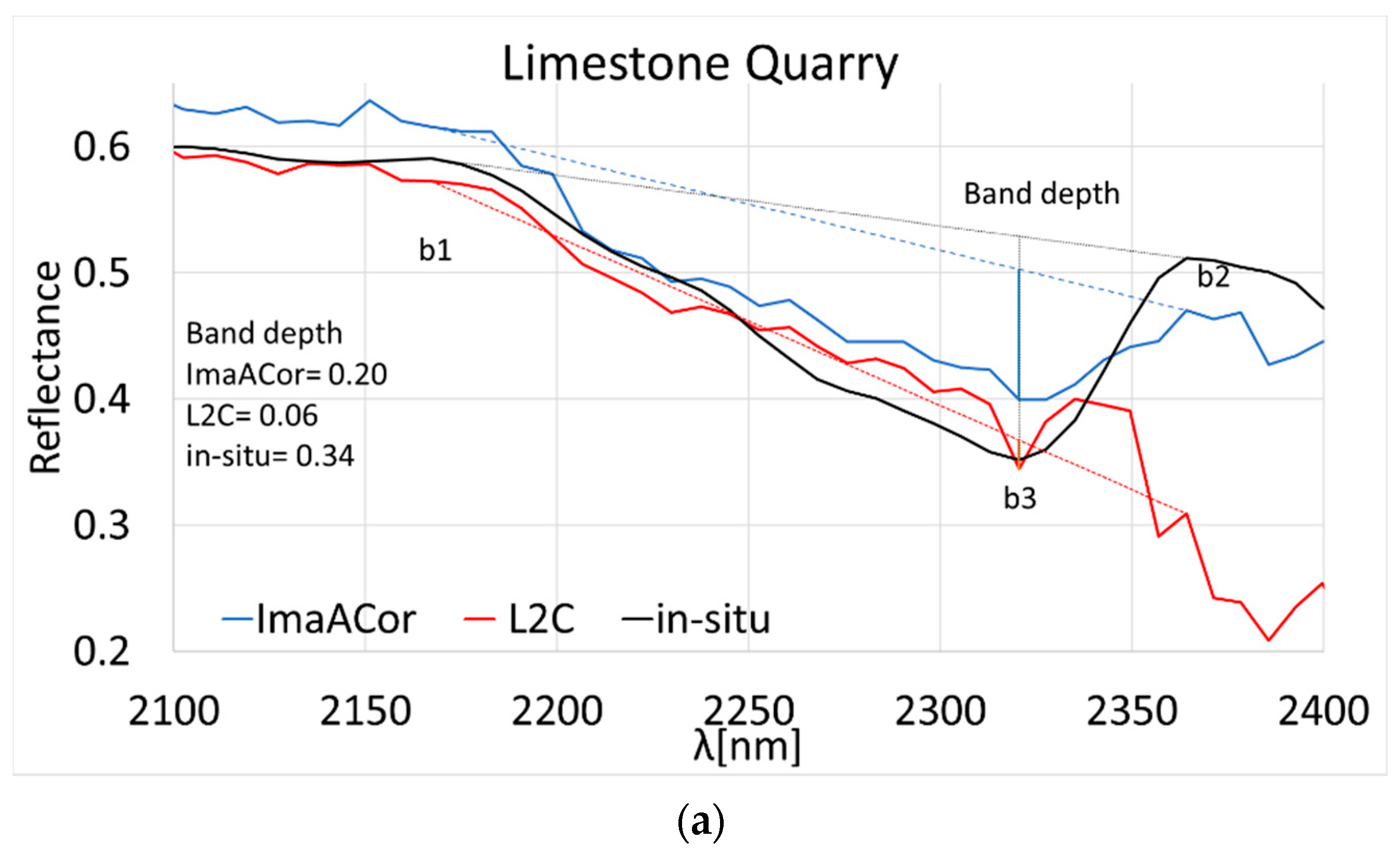
Model	Limestone Quarry	Airfield Strip	NPV	Paved Square
ImaACor	7	7	12	10
L2C	15	10	17	19

.

Table 6 shows the RRMSE values obtained for the ImaACor processor, which are very low.

From Figure 10 it emerges that this was mainly due to the blue end of the spectrum and to the bands above 2320 nm, since for the rest of the spectral range there was a good general agreement between L2C, ImaACOR, and the reference reflectance spectra of all targets.

The anomalous decrease in the values above 2320 nm was probably due to the L2C atmospheric correction procedure, as the ImaACor spectra were obtained starting from the same L1C images, unless the L2C image was processed starting from an LC1 image other than the distributed one. The lowered L2C reflectance values above 2320 nm caused the flattening of an important spectral feature between 2170 nm and 2370 nm, characteristic of the calcareous covers, which could prevent a correct classification of these materials. Figure 11 shows this effect for both the limestone quarry and the paved square. To quantify this flattening effect, the band depth values were computed for the bands b1 = 2175 nm, b2 = 2364 nm, and b3 = 2320 nm, corresponding to the two edges and to the minimum of the mentioned spectral feature, respectively. As expected, the band depth of the L2C reflectance spectra was significantly lower, being 0.06 for the limestone quarry, versus the 0.34 of the in-situ measurements and the 0.20 of the ImaACor, and −0.03 for the paved square, versus the 0.29 of the in situ reference and the 0.23 of the ImaACor.

4. Conclusions

This research aimed to evaluate the performance of the PRISMA hyperspectral mission in terms of the radiance (L1) and the reflectance (L2) standard products as collected for the rural area of Pignola in the Southern Apennines (Italy). Moreover, the first assessment of the SNR was performed with an image-based technique. This work did not aim to retrieve updated calibration coefficients for the PRISMA spectroradiometer, but it provided a quantitative performance assessment (i.e., by R2, RMSE, RRMSE, and RMAD) of the L1 and L2 data products for a rural area typical of the Southern Italy Apennine territory. To this end, from October 2019 to July 2021, we collected atmospheric characteristics and profiles (T, RH, and extinction @550 nm), as well as the radiances and reflectances of the principal land-cover types (targets ranging from bare soil to limestone quarry, including green vegetation and non-photosynthetic vegetation (crop residues) contemporary with the seven PRISMA acquisitions).

The PRISMA L1 radiance data compared to simulated data showed R² values higher than 0.98 and an average RRMSE value of 12.5%. Moreover, the RMAD between PRISMA L1 radiance and simulated TOA were usually about 5% up to the SWIR region, while from wavelengths higher than 2350nm the differences appeared greater than 10%.

The analysis of the reflectance standard products (version L2C_5.2.0) highlighted the presence of excessively low reflectance values for bands higher than 2300 nm, de facto determining the flattening of important spectral features in the far SWIR region, such as the limestone spectral features, which could make it difficult to recognize them on the standard L2C images. Moreover, the PRISMA images showed a residual coherent horizontal pattern of noise and a diagonal pattern from about 630 lines, with periodic disturbance at about 0.3–0.4 cycles/pixel that was present in all the analyzed images. SNR, as retrieved with an image-based technique from the Pignola images, showed values comparable with the actual observations obtained by Leonardo S.p.A., as reported in Table 1.

The overall results indicate that the fully equipped Pignola fiducial test site could provide a useful instrumented framework to evaluate the performance of PRISMA, and that the standard products L1 and L2 are suitable for the retrieval of biophysical parameters. On the other hand, the identified residual pattern noise requires the analysis of a more extensive dataset to define a robust correction algorithm to minimize the effect of this spatial pattern disturbance on parameter retrieval. This analysis is not exhaustive, and it is not intended to be a substitute for the utility of international calibration sites.

Further studies should include a wider range of land-cover types and spectral features in different environmental contexts.

References

- Loizzo, R.; Daraio, M.; Guarini, R.; Longo, F.; Lorusso, R.; Dini, L.; Lopinto, E. PRISMA mission status and perspective. In Proceedings of the IGARSS IEEE International Geoscience and Remote Sensing Symposium, Yokohama, Japan, 28 July–2 August 2019; pp. 4503–4506. [Google Scholar]
- Guanter, L.; Kaufmann, H.; Segl, K.; Foerster, S.; Rogass, C.; Chabrillat, S.; Kuester, T.; Hollstein, A.; Rossner, G.; Chlebek, C.; et al. The EnMAP Spaceborne Imaging Spectroscopy Mission for Earth Observation. Remote Sens. 2015, 7, 8830–8857. [Google Scholar] [CrossRef] [Green Version]
- Green, R.O.; Mahowald, N.; Ung, C.; Thompson, D.R.; Bator, L.; Bennet, M.; Zan, J. The earth surface mineral dust source investigation: An earth science imaging spectroscopy mission. In Proceedings of the 2020 IEEE Aerospace Conference, Big Sky, MT, USA, 7–14 March 2020; IEEE Computer Society: Big Sky, MT, USA, 2020. [Google Scholar]
- Lee, C.M.; Cable, M.L.; Hook, S.J.; Green, R.O.; Ustin, S.L.; Mandl, D.J.; Middleton, E.M. An introduction to the NASA Hyperspectral InfraRed Imager (HyspIRI) mission and preparatory activities. Remote Sens. Environ. 2015, 167, 6–19. [Google Scholar] [CrossRef]
- Matsunaga, T.; Iwasaki, A.; Tsuchida, S.; Iwao, K.; Tanii, J.; Kashimura, O.; Tachikawa, T. HISUI status toward FY2019 launch. In Proceedings of the International Geoscience and Remote Sensing Symposium (IGARSS), Valencia, Spain, 22–27 July 2018; pp. 160–163. [Google Scholar]
- Green, R.O.; Thompson, D.R.; EMIT Team. NASA’s Earth Surface Mineral Dust Source Investigation: An Earth Venture Imaging Spectrometer Science Mission. In Proceedings of the 2021 IEEE International Geoscience and Remote Sensing Symposium IGARSS, Bruxelles, Belgium, 11–16 July 2021; pp. 119–122. [Google Scholar]
- Müller, R.; Avbelj, J.; Carmona, E.; Eckardt, A.; Gerasch, B.; Graham, L.; Walter, I. The new hyperspectral sensor DESIS on the multi-payload platform muses installed on the ISS. Int. Arch. Photogramm. Remote Sens. Spat. Inf. Sci. 2016, 41, 461–467. [Google Scholar] [CrossRef] [Green Version]
- Rast, M.; Painter, T.H. Earth Observation Imaging Spectroscopy for Terrestrial Systems: An Overview of Its History, Techniques, and Applications of Its Missions. Surv. Geophys. 2019, 40, 303–331. [Google Scholar] [CrossRef]
- Nieke, J.; Rast, M. Towards the Copernicus Hyperspectral Imaging Mission For The Environment (CHIME). In Proceedings of the IGARSS 2018—2018 IEEE International Geoscience and Remote Sensing Symposium, Valencia, Spain, 22–27 July 2018; pp. 157–159. [Google Scholar]
- Feingersh, T.; Dor, E.B. SHALOM–A commercial hyperspectral space mission. In Optical Payloads for Space Missions; Qian, S.-E., Ed.; Wiley Online Library: Hoboken, NJ, USA, 2015; pp. 247–263. ISBN 9781118945179. [Google Scholar]
- Italian Space Agency Home Page. Available online: https://www.asi.it/en/2021/06/prisma-second-generation-psg-the-survey-for-the-future-of-hyperspectral-earth-observation-from-space/ (accessed on 7 February 2022).
- Pignatti, S.; Casa, R.; Laneve, G.; Li, Z.; Liu, L.; Marzialetti, P.; Mzid, N.; Pascucci, S.; Silvestro, P.C.; Tolomio, M.; et al. Sino–EU Earth Observation Data to Support the Monitoring and Management of Agricultural Resources. Remote Sens. 2021, 13, 2889. [Google Scholar] [CrossRef]
- Castaldi, F.; Palombo, A.; Pascucci, S.; Pignatti, S.; Santini, F.; Casa, R. Reducing the Influence of Soil Moisture on the Estimation of Clay from Hyperspectral Data: A Case Study Using Simulated PRISMA Data. Remote Sens. 2015, 7, 15561–15582. [Google Scholar] [CrossRef] [Green Version]
- Mzid, N.; Castaldi, F.; Tolomio, M.; Pascucci, S.; Casa, R.; Pignatti, S. Evaluation of Agricultural Bare Soil Properties Retrieval from Landsat 8, Sentinel-2 and PRISMA Satellite Data. Remote Sens. 2022, 14, 714. [Google Scholar] [CrossRef]
- Taramelli, A.; Tornato, A.; Magliozzi, M.L.; Mariani, S.; Valentini, E.; Zavagli, M.; Costantini, M.; Nieke, J.; Adams, J.; Rast, M. An Interaction Methodology to Collect and Assess User-Driven Requirements to Define Potential Opportunities of Future Hyperspectral Imaging Sentinel Mission. Remote Sens. 2020, 12, 1286. [Google Scholar] [CrossRef] [Green Version]
- Pignatti, S.; Amodeo, A.; Mona, L.; Palombo, A.; Pascucci, S.; Rosoldi, M.; Santini, F.; Casa, R.; Laneve, G. Evaluation of the PRISMA Hyperspectral Radiance Data: The PRISCAV Project Activities in the Basilicata Region (Southern Italy). In Proceedings of the IGARSS IEEE International Geoscience and Remote Sensing Symposium, Bruxelles, Belgium, 11–16 July 2021; pp. 1390–1393. [Google Scholar]
- Cogliati, S.; Sarti, F.; Chiarantini, L.; Cosi, M.; Lorusso, R.; Lopinto, E.; Miglietta, F.; Genesio, L.; Guanter, L.; Damm, A.; et al. The PRISMA imaging spectroscopy mission: Overview and first performance analysis. Remote Sens. Environ. 2021, 262, 112499. [Google Scholar] [CrossRef]
- Guanter, L.; Irakulis-Loitxate, I.; Gorroño, J.; Sánchez-García, E.; Cusworth, D.H.; Varon, D.J.; Cogliati, S.; Colombo, R.R. Mapping methane point emissions with the PRISMA spaceborne imaging spectrometer. Remote Sens. Environ. 2021, 265, 112671. [Google Scholar] [CrossRef]
- Romaniello, V.; Silvestri, M.; Buongiorno, M.F.; Musacchio, M. Comparison of PRISMA Data with Model Simulations, Hyperion Reflectance and Field Spectrometer Measurements on ‘Piano delle Concazze’ (Mt. Etna, Italy). Sensors 2020, 20, 7224. [Google Scholar] [CrossRef] [PubMed]
- Fox, N. A Guide to Expression of Uncertainty of Measurements. Available online: http://qa4eo.org/docs/QA4EO-QAEO-GEN-DQK-006_v4.0.pdf (accessed on 7 February 2022).
- Niro, F.; Goryl, P.; Dransfeld, S.; Boccia, V.; Gascon, F.; Adams, J.; Themann, B.; Scifoni, S.; Doxani, G. European Space Agency (ESA) Calibration/Validation Strategy for Optical Land-Imaging Satellites and Pathway towards Interoperability. Remote Sens. 2021, 13, 3003. [Google Scholar] [CrossRef]
- Bouvet, M.; Thome, K.; Berthelot, B.; Bialek, A.; Czapla-Myers, J.; Fox, N.P.; Goryl, P.; Henry, P.; Ma, L.; Marcq, S.; et al. RadCalNet: A Radiometric Calibration Network for Earth Observing Imagers Operating in the Visible to Shortwave Infrared Spectral Range. Remote Sens. 2019, 11, 2401. [Google Scholar] [CrossRef] [Green Version]
- Heller Pearlshtien, D.; Pignatti, S.; Greisman-Ran, U.; Ben-Dor, E. PRISMA sensor evaluation: A case study of mineral mapping performance over Makhtesh Ramon, Israel. Int. J. Remote Sens. 2021, 42, 5882–5914. [Google Scholar] [CrossRef]
- Jeffrey Czapla-Myers, J.; Ong, L.; Thome, K.; McCorkel, J. Validation of EO-1 hyperion and advanced land imager using the radiometric calibration test site at Railroad Valley, Nevada. IEEE J. Sel. Top Appl. Earth Obs. Remote Sens. 2015, 9, 816–826. [Google Scholar] [CrossRef]
- Santini, F.; Palombo, A. Physically Based Approach for Combined Atmospheric and Topographic Corrections. Remote Sens. 2019, 11, 1218. [Google Scholar] [CrossRef] [Green Version]
- Coppo, P.; Brandani, F.; Faraci, M.; Sarti, F.; Dami, M.; Chiarantini, L.; Ponticelli, B.; Giunti, L.; Fossati, E.; Cosi, M. Leonardo spaceborne infrared payloads for Earth observation: SLSTRs for Copernicus Sentinel 3 and PRISMA hyperspectral camera for PRISMA satellite. Appl. Opt. 2020, 59, 6888. [Google Scholar] [CrossRef]
- Madonna, F.; Amodeo, A.; Boselli, A.; Cornacchia, C.; Cuomo, V.; D’Amico, G.; Giunta, A.; Mona, L.; Pappalardo, G. CIAO: The CNR-IMAA advanced observatory for atmospheric research. Atmos. Meas. Tech. 2011, 4, 1191–1208. [Google Scholar] [CrossRef] [Green Version]
- Berk, A.G.P.A.; Anderson, G.P.; Acharya, P.K.; Chetwynd, J.H.; Bernstein, L.S.; Shettle, E.P.; Matthew, M.W.; Adler-Golden, S.M. MODTRAN4 User’s Manual; Air Force Research Laboratory: Bedford, MA, USA, 1999. [Google Scholar]
- Vermote, E.F.; Tanré, D.; Deuze, J.L.; Herman, M.; Morcette, J.J. Second simulation of the satellite signal in the solar spectrum, 6S: An. overview. IEEE Trans. Geosci. Remote Sens. 1997, 35, 675–686. [Google Scholar] [CrossRef] [Green Version]
- Bhatt, R.; Doelling, D.R.; Coddington, O.; Scarino, B.; Gopalan, A.; Haney, C. Quantifying the Impact of Solar Spectra on the Inter-Calibration of Satellite Instruments. Remote Sens. 2021, 13, 1438. [Google Scholar] [CrossRef]
- Papagiannopoulos, N.; Mona, L.; Alados-Arboledas, L.; Amiridis, V.; Baars, H.; Binietoglou, I.; Bortoli, D.; D’Amico, G.; Giunta, A.; Guerrero-Rascado, J.L.; et al. CALIPSO climatological products: Evaluation and suggestions from EARLI-NET. Atmos. Chem. Phys. 2016, 16, 2341–2357. [Google Scholar] [CrossRef] [Green Version]
- Papagiannopoulos, N.; Mona, L.; Amodeo, A.; D’Amico, G.; Gumà Claramunt, P.; Pappalardo, G.; Alados-Arboledas, L.; Guerrero-Rascado, J.L.; Amiridis, V.; Kokkalis, P.; et al. An automatic observation-based aerosol typing method for EARLINET. At-mos. Chem. Phys. 2018, 18, 15879–15901. [Google Scholar] [CrossRef] [Green Version]
- Richter, K.; Atzberger, C.; Hank, T.; Mauser, W. Derivation of biophysical variables from Earth Observation data: Validation and statistical measures. J. Appl. Remote Sens. 2012, 6, 063557. [Google Scholar] [CrossRef]
- Chang, C.-I.; Du, Q. Estimation of number of spectrally distinct signal sources in hyperspectral imagery. IEEE Trans. Geosci. Remote Sens. 2004, 42, 608–619. [Google Scholar] [CrossRef] [Green Version]
- Thompson, D.R.; Braverman, A.; Brodrick, P.G.; Candela, A.; Carmon, N.; Clark, R.N.; Connelly, D.; Green, R.O.; Kokaly, R.F.; Li, L.; et al. Quantifying uncertainty for remote spectroscopy of surface composition. Remote Sens. Environ. 2020, 247, 111898. [Google Scholar] [CrossRef]
- Thompson, D.R.; Babu, K.N.; Braverman, A.J.; Eastwood, M.L.; Green, R.O.; Hobbs, J.M.; Jewell, J.B.; Kindel, B.; Massie, S.; Mishra, M.; et al. Optimal estimation of spectral surface reflectance in challenging atmospheres. Remote Sens. Environ. 2019, 232, 111258. [Google Scholar] [CrossRef]
- PRISMA Products Specification Document Issue 2.3 Date 12 March 2020. Italian Space Agency. Available online: http://prisma.asi.it/missionselect/docs/PRISMA%20Product%20Specifications_Is2_3.pdf (accessed on 7 February 2022).
- Cooley, T.; Anderson, G.P.; Felde, G.W.; Hoke, M.L.; Ratkowski, A.J.; Chetwynd, J.H.; Gardner, J.A.; Adler-Golden, S.M.; Matthew, M.W.; Berk, A.; et al. FLAASH, a MODTRAN4-based atmospheric correction algorithm, its application and validation. In Proceedings of the IEEE International Geoscience and Remote Sensing Symposium, Toronto, ON, Canada, 24–28 June 2002; Volume 3, pp. 1414–1418. [Google Scholar]
- Palombo, A.; Santini, F. ImaACor: A Physically Based Tool for Combined Atmospheric and Topographic Corrections of Remote Sensing Images. Remote Sens. 2020, 12, 2076. [Google Scholar] [CrossRef]
- Acito, N.; Diani, M.; Corsini, G. Signal-Dependent Noise Modeling and Model Parameter Estimation in Hyperspectral Images. IEEE Trans. Geosci. Remote Sens. 2011, 49, 2957–2971. [Google Scholar] [CrossRef]
- Fu, P.; Sun, X.; Sun, Q. Hyperspectral Image Segmentation via Frequency-Based Similarity for Mixed Noise Estimation. Remote Sens. 2017, 9, 1237. [Google Scholar] [CrossRef] [Green Version]
- Bernstein, R.; Lotspoech, J.B.; Myers, H.J.; Kolsky, H.G.; Lees, R.D. Analysis And Processing of LANDSAT-4 Sensor Data Using Advanced Image Processing Techniques And Technologies. IEEE Trans. Geosci. Remote Sens. 1984, GE-22, 192–221. [Google Scholar] [CrossRef]
- Helder, D.L.; Ruggles, T.A. Landsat thematic mapper reflective-band radiometric artifacts. IEEE Trans. Geosci. Remote Sens. 2004, 42, 2704–2716. [Google Scholar] [CrossRef]