Landsat-8 Sea Ice Classification Using Deep Neural Networks

Abstract

Knowing the location and type of sea ice is essential for safe navigation and route optimization in ice-covered areas. In this study, we developed a deep neural network (DNN) for pixel-based ice Stage of Development classification for the Baltic Sea using Landsat-8 optical satellite imagery to provide up-to-date ice information for Near-Real-Time maritime applications. In order to train the network, we labeled the ice regions shown in the Landsat-8 imagery with classes from the German Federal Maritime and Hydrographic Agency (BSH) ice charts. These charts are routinely produced and distributed by the BSH Sea Ice Department. The compiled data set for the Baltic Sea region consists of 164 ice charts from 2014 to 2021 and contains ice types classified by the Stage of Development. Landsat-8 level 1 (L1b) images that could be overlaid with the available BSH ice charts based on the time of acquisition were downloaded from the United States Geological Survey (USGS) global archive and indexed in a data cube for better handling. The input variables of the DNN are the individual spectral bands: aerosol coastal, blue, green, red and near-infrared (NIR) out of the Operational Land Imager (OLI) sensor. The bands were selected based on the reflectance and emission properties of sea ice. The output values are 4 ice classes of Stage of Development and Ice Free. The results obtained show significant improvements compared to the available BSH ice charts when moving from polygons to pixels, preserving the original classes. The classification model has an accuracy of 87.5% based on the test data set excluded from the training and validation process. Using optical imagery can therefore add value to maritime safety and navigation in ice- infested waters by high resolution and real-time availability. Furthermore, the obtained results can be extended to other optical satellite imagery such as Sentinel-2. Our approach is promising for automated Near-Real-Time (NRT) services, which can be deployed and integrated at a later stage at the German Aerospace Center (DLR) ground station in Neustrelitz.

1. Introduction

In seasonally ice-covered locations, ice conditions vary widely both spatially and temporally, leading to uncertainties and problems in maritime procedures [1]. In the northern Baltic sea, winter navigation is a difficult but routine operation; incidents resulting in vessel losses and oil spills have occurred and may continue to occur in the future [2]. Sea ice classification information contributes to safe navigation and route optimization and reduces the risk for navigation in ice-covered waters. It is worthwhile to prepare routes for ships traveling long distances in the ice that reduce fuel consumption and travel time and reduce the risk of running into dangerous places or becoming stacked in the ice [3]. A Near-Real-Time (NRT) ice classification would be extremely useful for this route optimization due to the changing ice conditions.

For this classification, satellite systems are widely used today and have a firm place especially in the maritime domain. Synthetic Aperture Radar (SAR) sensors are the most used image source for maritime situational awareness; especially sea ice classification [4]. Optical systems can make a valuable contribution as cooperative sensors. The variety of available spectral channels is more advantageous for information extraction as opposed to radar remote sensing [5]. In the context of sea ice classification, optical sensors provide valuable information based on the reflectance and emission properties of the surface such as spectral albedo which is very sensitive to sea ice thickness whose structure varies greatly [6]. Even though possible cloud cover and low sun elevation in northern latitudes limit the use of optical data seasonally, the high resolution and timeliness can add valuable information when available. This study relies on Landsat-8, as a way to provide additional information for classification of sea ice in order to reduce the temporal gaps for providing updated ice information for NRT applications.

Several methods of ice classification using optical satellite imagery have been developed to approach this problem. Richter et al. uses a simple classification using the normalized difference snow index (NDSI) [7], which combines different regions of the electromagnetic spectrum; this method only distinguishes ice from water but it is convenient for creating ice masks which we used later in this study. Traditional algorithms such as Support Vector Machines (SVM) or decision trees can also be used for hyperspectral data classification [5]. These methods are very accurate but not appropriate for extracting deeper characteristics [8]. Artificial Intelligence methods such as Deep Neural Networks (DNNs) have shown impressive results in addressing remote sensing problems [9]. Han et al. propose a classification based on remote sensing data fusion between SAR and optical sources and apply a Convolutional Neural Network (CNN) for the optical data for a deep feature extraction with a classification accuracy of 95.69% [8]. However, the convolutional computation is a technical challenge for NRT applications due to its time consumption [10], especially in large areas as the Baltic Sea. DNN are efficient [11] and can also be used for pixel-based classification [12].

Alongside from an efficient classification, an NRT process is proposed to retrieve the ice classification results. The German Aerospace Center (DLR) ground station in Neustrelitz, where this work is being conducted, provides the whole infrastructure for receiving and processing satellite images and delivering them as fast as feasible [13].

The main contributions of our proposed model are described below:

• In terms of computational power, we propose a DNN-based algorithm that is very light compared to the commonly used CNN models and optimally suited for an NRT maritime service. The model is high performing, accurate and convenient to apply on large images. The required ice classification for the requested areas of the Baltic Sea will be automatically derived directly after reception and processing of the Landsat-8 imagery at the DLR ground station Neustrelitz.
• We show how a data cube can be extremely useful to store satellite imagery and retrieve data without the need for manual work. This is also useful to combine different images for training data extraction. In addition, the data cube allows preliminary analysis to identify useful training days with near-clear skies and sufficient ice coverage. It is also possible to extend the data cube with additional products such as Sentinel-2.
• We demonstrate how machine learning can adapt to imperfect training data and still produce good results. The use of BSH ice charts was limited because they did not perfectly match all image regions. The incoherence is because they were not created with Landsat-8 imagery and were obtained at different acquisition times.
• Despite these drawbacks, the model has learned to make a valid distinction between ice and water and to make a classification that is consistent with the training data. Visual inspection shows that ice classification and mapping are consistent, which can be further improved by training more specific ice classes. An overall accuracy of 87.5 percent was achieved.

The rest of this paper is organized as follows: The second section describes the process to create the training data assembled to train the network. The third section presents in detail the methodology of the DNN. In the fourth section, the findings of the obtained results of this methodology are discussed, including the presentation of selected results.

2. Data

2.1. BSH Ice Charts

The quality of the training data is of highest importance in determining the quality of the classification result obtained. Nowadays, sea ice information is provided through various portals to support navigation in ice-covered waters. One of these providers is the Ice Service department of the German Federal Maritime and Hydrographic Agency (Bundesamt für Seeschifffahrt und Hydrographie, BSH) in Rostock, Germany. Data from various satellites and coastal ice observers are used to create these manually produced ice charts.

These BSH ice maps are the initial source of information to annotate ice locations on Landsat-8 images to create the training data for a pixel-based sea ice classifier. They consist of GIS vector maps (GML) which contain the Ice Stage of Development (ICESOD) codes. In total, 164 BSH ice charts from 2014 to 2021 were available for the study area.

Table 1. BSH Ice chart—Stage of Development classes.

ICESOD	Description
1	Ice Free
85	Gray—White Ice (15 to <30 cm)
88	Thin First Year Ice Stage 1 (30 to <50 cm)
89	Thin First Year Ice Stage 2 (50 to <70 cm)
91	Medium First Year Ice (70 to 120 cm)

summarizes the classes, their code values and the corresponding meaning with respect to the ice thickness (value in brackets) used for this study. The ice types correspond to the dominant ice type in terms of partial ice concentration.

2.2. Landsat-8 Data

Landsat-8 is an Earth observation satellite, operated by a collaboration between NASA and USGS [14]. One of the sensors on board of the satellite is the Operational Land Imager (OLI), which uses 9 bands in the spectrum of visible light and Near Infrared. It is based on the wide swath imaging mode; the single scene size is 185 × 180 km which allows the specific monitoring of wide marine areas. We downloaded the Landsat-8 imagery that overlapped the BSH ice charts with a valid time difference of one day at most and a cloud coverage less than 60%. In total, 565 Landsat-8 scenes were obtained for the Baltic Sea region.

2.3. Data Handling

Due to the large amount of imagery that met the training data criteria, the Landsat-8 images were stored in a data cube (Open Data Cube, ODC) [15]. As the name already suggests, the data cube is an extension of a two-dimensional matrix where the data sets are arranged as elements of a multidimensional cube. In the context of modeling, the use of a data cube has several advantages. For example, data can be retrieved by various parameters such as date or spatial region, which saves time by eliminating the need to manually select and search for images. This is also very convenient for processing data from multiple days. In addition, the data cube also allows for initial analysis to identify the images with almost clear sky and sufficient ice cover. It is also possible to retrieve the data from several Landsat-8 images for training the DNN. Figure 1 illustrates a visualization of the data cube with multiple Landsat-8 images overlapping the BSH ice charts and an OpenStreetMap base map. The Landsat-8 images (diagonal strip on the left side) are displayed using a combination of bands (Green, Red, NIR) that shows a false color representation to facilitate the differentiation of the ice from the water and the land.

The scenes included in the data cube correspond to the calibrated raw level 1 data. A top of atmosphere reflectance (TOA) calculation was included to be computed on the fly and it is described in the following equations [14]:

$${\rho }_{\lambda }\text{′}=M_P*Q_{CAL}+A_P$$

(1)

where

${\rho }_{\lambda }\text{′}$	TOA Planetary Spectral reflectance, without correction for solar angle. (Unitless)
$M_P$	Reflectance multiplicative scaling factor for the band
$Q_{CAL}$	Level 1 pixel value in DN
$A_P$	Reflectance additive scaling factor for the band

$${\rho }_{\lambda }=\frac{{\rho }_{\lambda }’}{\cos \left({\theta }_{SZ}\right)}=\frac{{\rho }_{\lambda }’}{\sin \left({\theta }_{SE}\right)}$$

(2)

where

${\rho }_{\lambda }$	TOA Planetary Spectral reflectance
${\theta }_{SE}$	Local sun elevation angle
${\theta }_{SZ}$	Local solar zenith angle

The TOA calculation standardizes the input data since the albedo range is usually between 0 and 1 which is unitless and represents the ratio of solar radiation that is reflected [6].

Additional atmospheric corrections would improve the image quality but also require external datasets [16]. These corrections were omitted to reduce the computational cost of the algorithm and because it is intended for use in NRT operations which do not allow external data at the time of reception.

3. Methods

3.1. Overview

The methodology from collecting the Landsat-8 images to creating the DNN is presented in the following flowchart, see Figure 2.

3.2. Data Collection

The selection of the Landsat-8 spectral bands is based on the optical properties of sea ice. The stage of development of sea ice has a complex structure that affects its light reflection. The most common optical property to differentiate ice conditions is the albedo, defined as the fraction of the incident irradiance that is reflected [5]. The albedo value depends on the different stages of the sea ice, varying along the shortwave radiation portion of the electromagnetic spectrum. Figure 3 shows the different stages of development (first year ice, young gray ice, nilas, open water) and the influence of the type of surface on the reflection of light in different wavelengths.

The wavelength range presented in

Table 2. Landsat-8 bands.

Bands	Wavelength (nm)
Band 1—Coastal aerosol	430–450
Band 2—Blue	450–510
Band 3—Green	530–590
Band 4—Red	640–670
Band 5—Near Infrared (NIR)	850–880

can be divided in the first 5 bands of the Landsat-8 image. See Table 2.

Based on the characteristics of each channel, a combination of Landsat-8 spectral bands: Aerosol Coastal (1), Blue (2), Green (3), Red (4) and NIR (5) were chosen to create the training data sets. For the expected ice classification values, the codes were obtained from the corresponding BSH ice chart. All training data were extracted using the native resolution of 30 m provided by the sensor.

Training data were extracted by creating an ice mask from the Landsat-8 imagery. This mask was obtained using the Normalized Difference Snow Index [7], defined as follows:

$$\mathrm{NDSI}=\frac{{\rho }_{\lambda }\left(\mathrm{green}\right)-{\rho }_{\lambda }\left(\mathrm{SWIR}1\right)}{{\rho }_{\lambda }\left(\mathrm{green}\right)+{\rho }_{\lambda }\left(\mathrm{SWIR}1\right)}$$

(3)

The following threshold was applied:

$${\rho }_{\lambda }\left(\mathrm{blue}\right)>0.22\mathrm{and}\mathrm{NDSI}>0.6$$

(4)

To remove the land, an OpenStreetMap land mask has been applied. Figure 4 shows a result example.

The ice mask was overlaid with the BSH ice charts to create the training data using the ICESOD codes, Figure 5a. The polygons from the BSH charts were rasterized and a code was assigned to every pixel. Additional ice free values were retrieved using the water mask which is obtained by subtracting the ice mask from the inverted land mask, Figure 5b.

There was a selection process to identify images without cloud cover and sufficient ice to extract the training data. The BSH ice charts were selected to be as close to the selected day. The days and the coordinates used for the training are presented in

Table 3. Coordinates of training days.

Training Day	BSH Ice Chart Day	Bounding Box (WGS84)
22 March 2019	21 March 2019	Longitude (23.5, 25.5), Latitude (64, 66)
23 April 2019	24 April 2019	Longitude (21, 26), Latitude (63, 66)
16 April 2019	15 April 2019	Longitude (23, 25.5), Latitude (64, 65.8)
16 February 2021	16 February 2021	Longitude (24, 25.5), Latitude (64.5, 66)

.

A total of 60.715.461 input values (pixels) were extracted. Every input consists of 5 variables representing each band. The number of input samples (pixels) for every class can be seen in

Table 4. Stage of Development classes.

Class (ICESOD)	Number of Pixels	Total %
1: Ice Free	32,698,818	53.86
85: Gray-White Ice	3,222,135	5.31
88: Thin First Year Ice Stage 1	4,506,661	7.42
89: Thin First Year Ice Stage 2	10,387,946	17.11
91: Medium First Year Ice	9,899,901	16.31

.

The whole image data collection was split into 3 independent data sets. The first one was for training purposes, the second one was for validation and the last one was for testing. See

Table 5. Training, validation and test data sets.

Data set	Number of Pixels	Total %
Training	60,715,461	80
Validation	6,071,546	10
Test	6,071,547	10

.

The training data was exported to numpy compressed array format (npz) files that can be loaded into Tensorflow, a free and open-source software library for machine learning [18]. In this process, the spatial features are lost since the data are now in tabular form.

3.3. Deep Neural Network

A DNN based on an input layer, hidden layers and an output layer was trained using the completed and ready-to-use training and validation data sets. In our model, there are 4 hidden layers, each one with a depth of 40 nodes. The selection of the number of hidden layers and nodes is based on the experience of several tests with the aim of higher accuracy. The input layer has 5 nodes corresponding to the TOA from the subset of the 5 selected Landsat-8 spectral bands as described in the previous chapter. The output layer has 5 nodes corresponding to the ICESOD classes (1, 85, 88, 89 and 91).

The DNN uses a supervised learning algorithm to search for weight values that optimizes the linear and nonlinear relationships between the layers to solve complex problems [19]. The main objective of this DNN is to determine the ICESOD code that corresponds to the 5 top of atmosphere values (TOA) values presented in each pixel of the Landsat-8 image. Figure 6 shows the architecture of the DNN, programmed using Tensorflow.

The DNN uses the Gradient Descent optimization technique to train the machine learning model. This process minimizes the errors of the categorical cross-entropy loss function, appropriate for multiclass classification tasks [20]. The model is optimized through several iterations called epochs during the back propagation [21], a feed forward method that adjusts the weights by comparing training values with the expected output of the training samples [22]. For an efficient optimization, the Adaptive Moment Estimation (Adam) algorithm was applied to compute individual adaptive learning rates [23].

Between each layer of the network, the activation functions are defined. These nonlinear functions are needed in the neural network to separate the layers and manage complex functions [16]. For the input layer and the 4 hidden layers, the Rectified Liner Unit (ReLU) activation function is used. This function speeds up computation performance since the negative values are cropped, which reduces the number of activated neurons in the network and its derivative which is very simple [24]. For the final layer the SoftMax activation function was applied. This function calculates the probability distribution between the classes. Based on the SoftMax output, the final classification is done.

Table 6. Hyperparameters.

Input
Loss function	Categorical cross-entropy
Optimizer	Adam
Activation function	ReLU
Classification rule	SoftMax

presents the summary of hyperparameters used for this model.

4. Results and Discussion

4.1. Training Results

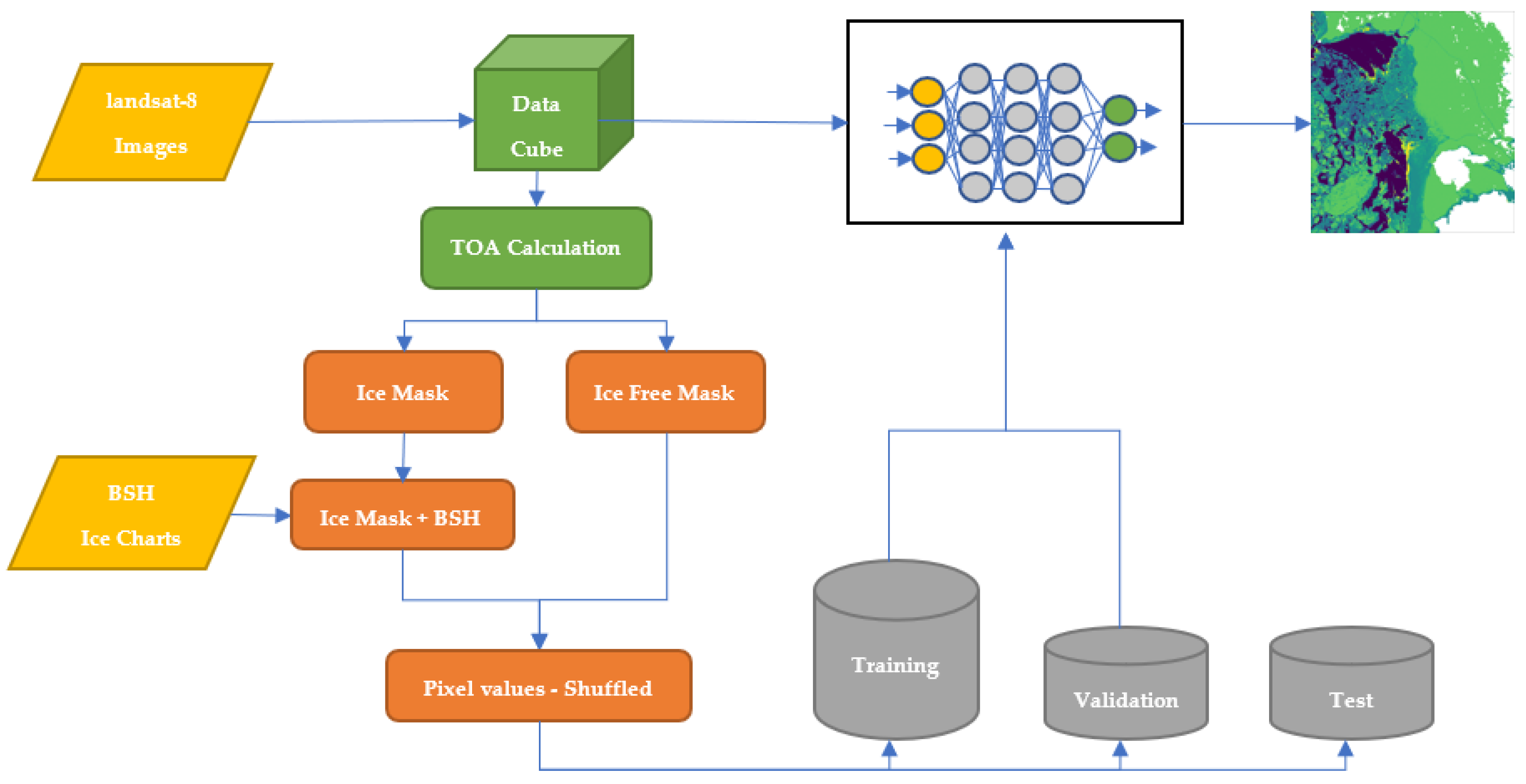
The model was trained in a virtual machine with the characteristics presented in

Table 7. Hardware used for the learning process.

Device	Hardware
Architecture	x86_64
GPU (X1)	Nvidia Tesla T4 16 GB RAM
Processor (X12)	Intel(R) Xeon(R) Gold 6154 CPU @ 3.00 GHz
Memory	32 GB RAM

. A batch size of 100,000 was selected to divide the training data set in chunks. An early stopping callback was applied; this stops the iteration process after each epoch in case the validation accuracy decreases two times in a row. Multiprocessing with 12 processors was deployed. The training time was 4 min and it was finished after 21 epochs.

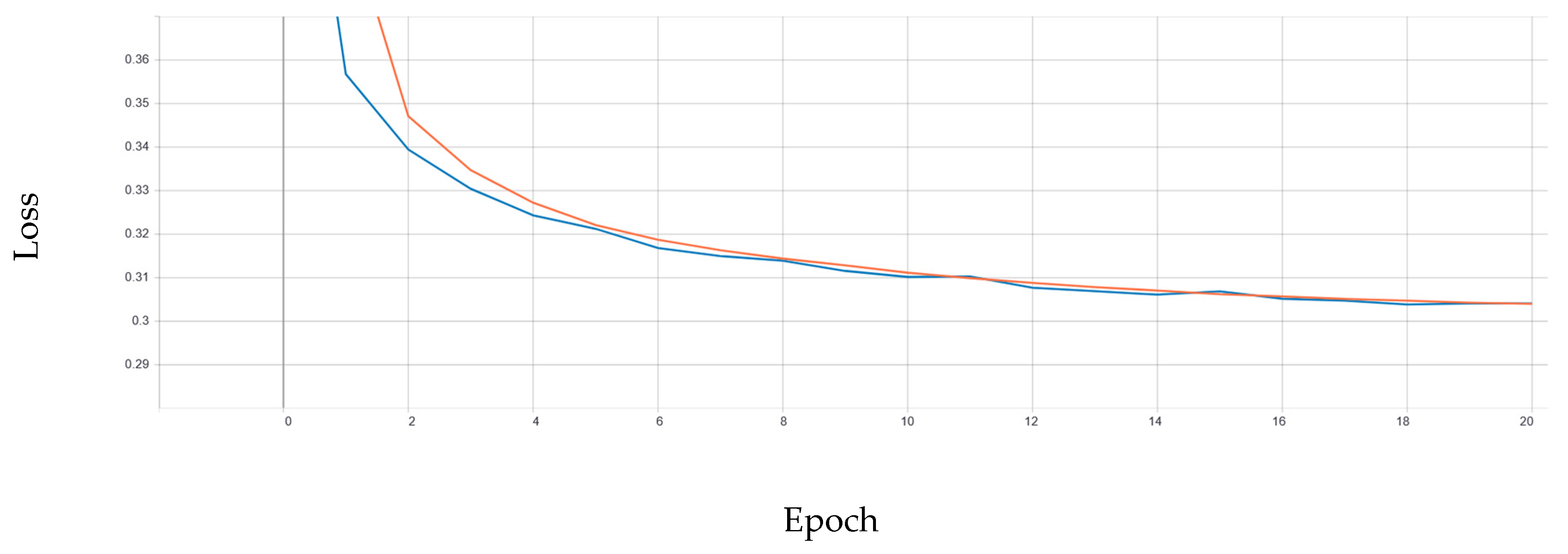
The training of the model has shown a purposeful behavior that can be seen in terms of the loss and accuracy. The decrease in the loss is presented in Figure 7. The increase in the accuracy is presented in Figure 8.

After the training was finished, the results of the model were validated using the dedicated test data set. This data set was not previously involved in the training process. The final loss and accuracy are 0.3043 and 0.8748, respectively, showing an overall successful training process.

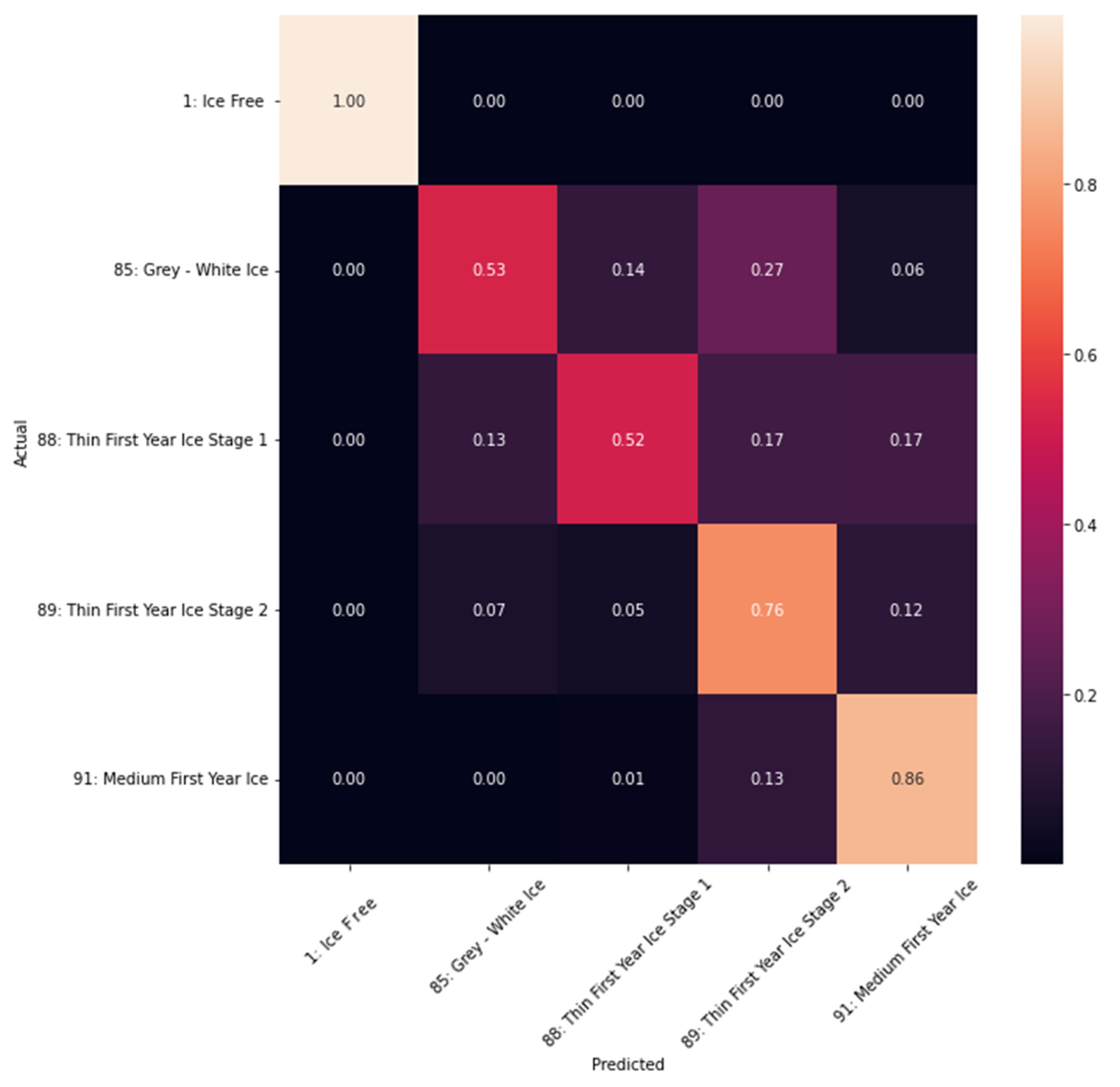
It is important to note that the training data set is imbalanced. Table 4 shows the sample size of different classes showing more data available for the classes of 1 (Ice Free), 89 (Thin First Year Ice Stage 2) and 91 (Medium First Year Ice) with little data for 85 (Gray-White Ice), and 88 (Thin First Year Ice Stage 1). The reason for this huge imbalance is caused by the nature of the ice represented in the ice charts used for the training. The accuracy of the different classes can be seen in the confusion matrix. The confusion matrix is a cross table that represents the accuracy between classes considered as ground truth (rows) and their predictions (columns) [25]. Figure 9 shows the confusion matrix used for the test data set. It can be seen that the accuracy is lower for the classes with less available training data, while the other classes with more data, show higher accuracy, especially Ice Free with a 100% of accuracy followed by 91 with 86% and 89 with 76%. Apparently, these classes have higher accuracy because their features are more presented in the data set. Balancing the dataset, that means, making all the classes to have the same proportion of the dataset while removing additional data, will produce a loss on the quality and quantity on the training, thus affecting the results. In this scenario, additional extraction of training data on 85 and 88 is suggested.

4.2. Graphics Results

For a visual validation, two types of outputs were generated, a Landsat-8 false color image (green, red and NIR) and an ice classification chart. The images with false color help to easily identify the ice from the water or land. On top of this layer, the BSH Ice charts were added, which worked as the features for extracting the training data. On the other hand, the ice classification charts are generated by the DNN using the selected five Landsat-8 bands. Figure 10, Figure 11, Figure 12, Figure 13, Figure 14, Figure 15, Figure 16 and Figure 17 show some examples.

4.3. Discussion

The DNN classification show very good results with the Landsat-8 imagery regarding the distinction between ice and no ice. The agreement with the BSH ice charts depends on the accuracy of each class related to the availability of training data as shown in the confusion matrix, see Figure 9. However, there is a clear improvement when moving from polygons to pixels while maintaining the original BSH classes. The first evaluation of the model results in an accuracy of 87.5%. This result is based on the test data set, which is not part of the training or validation data set.

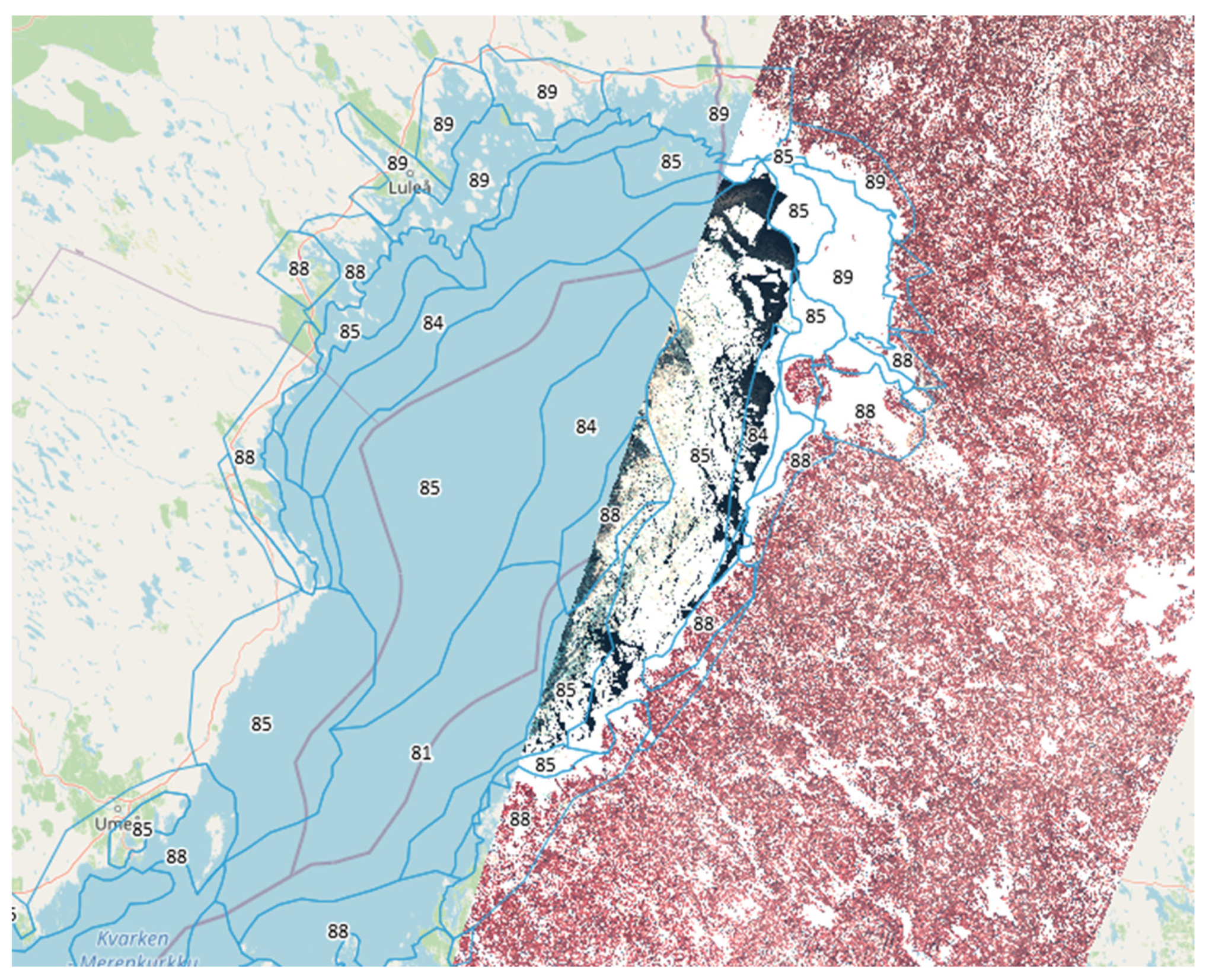
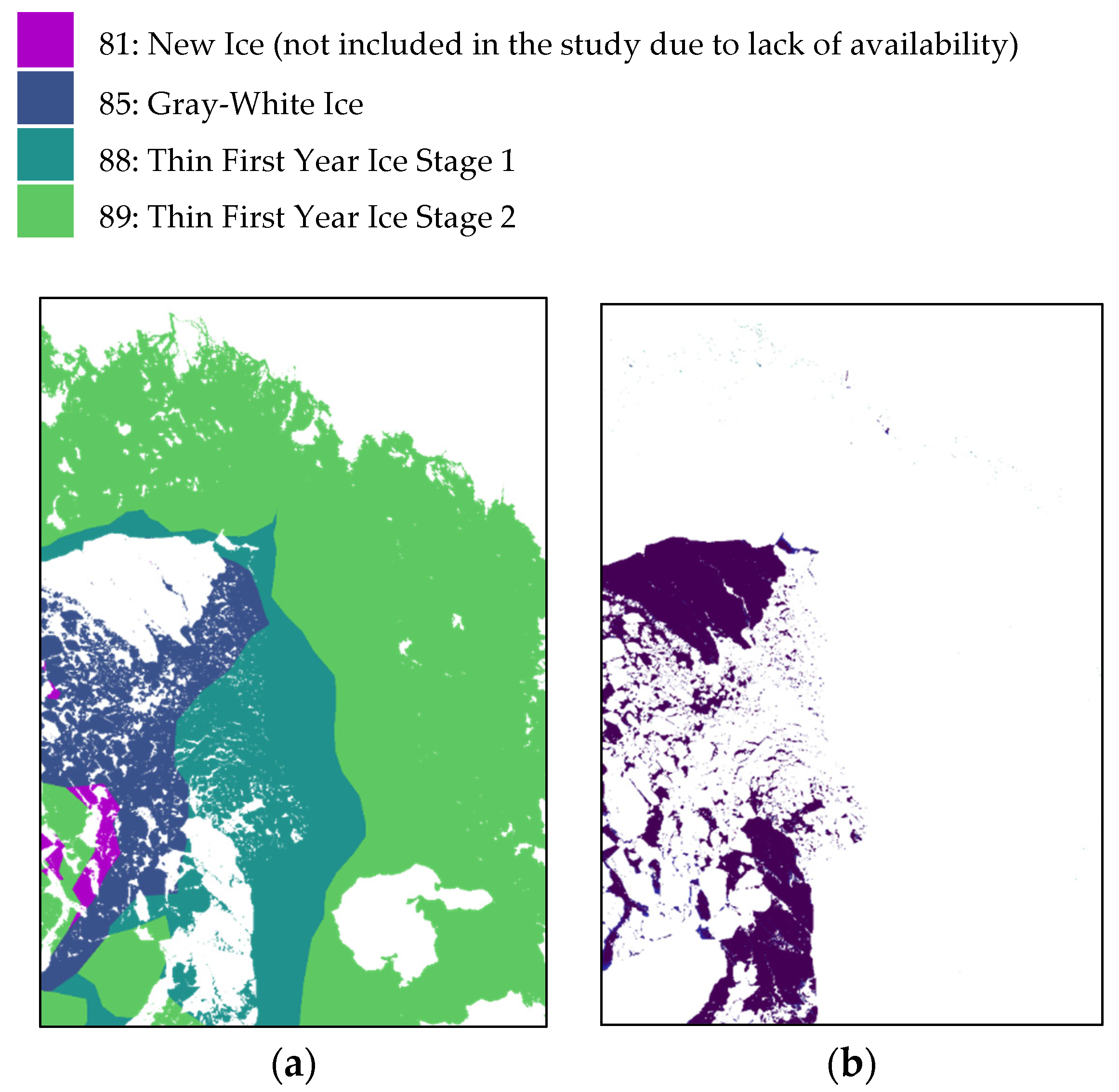
Figure 10 output shows a predominance of class 88 (Thin First Year Ice Stage 1) which corresponds to some polygons of the training data. In addition, the algorithm detects class 85 (Gray-White ice) which does not appear in the training data for this region.

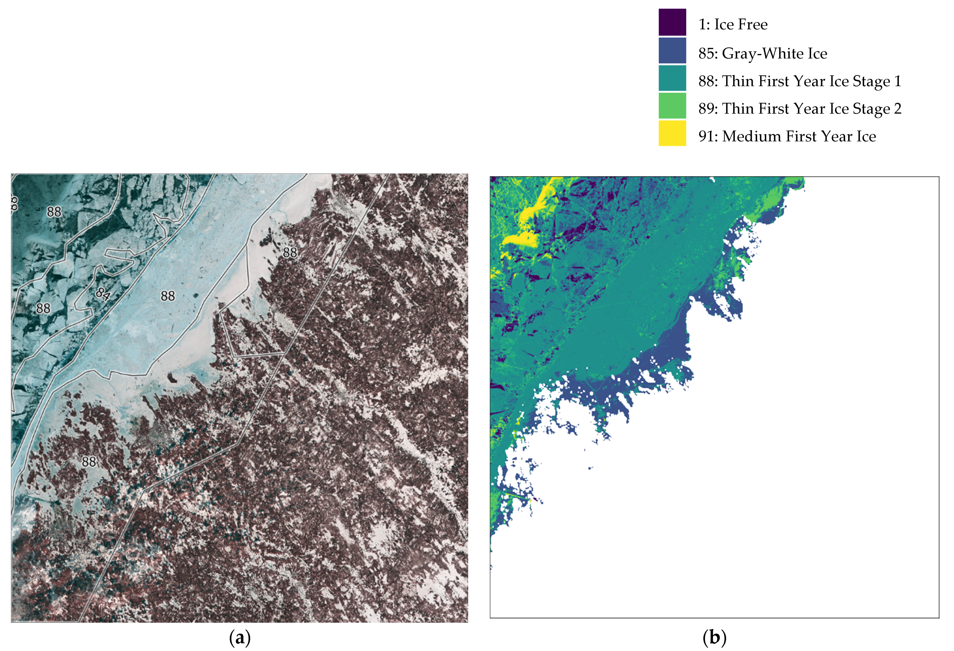
Figure 11 shows a good representation; there is a clear distinction between classes 88 (Thin First Year Ice Stage 1) and 89 (Thin First Year Ice Stage 2) and a smooth transition between 88 and 85. Class 91 is shown in some boundaries. Ice Free is clearly marked and some icebreaker vessel routes are also visible.

Figure 12 shows that the training polygons are shifted relative to the ice locations in the false color image. This difference occurs because the Landsat-8 image and the BSH ice chart differ by one day. Nevertheless, the algorithm distinguishes well between water and ice and the two classes most represented in the false color image (88 and 89) are therefore classified.

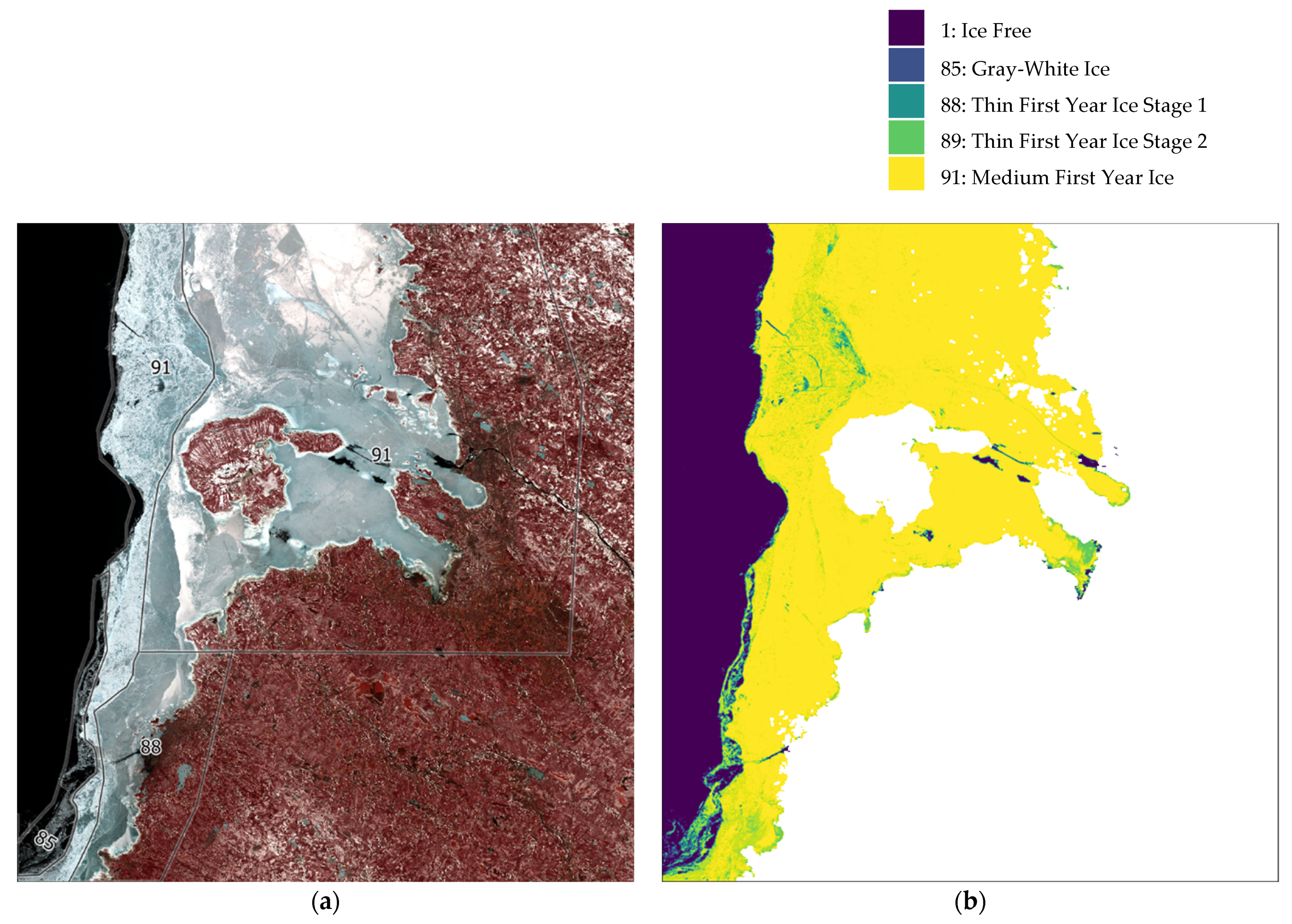
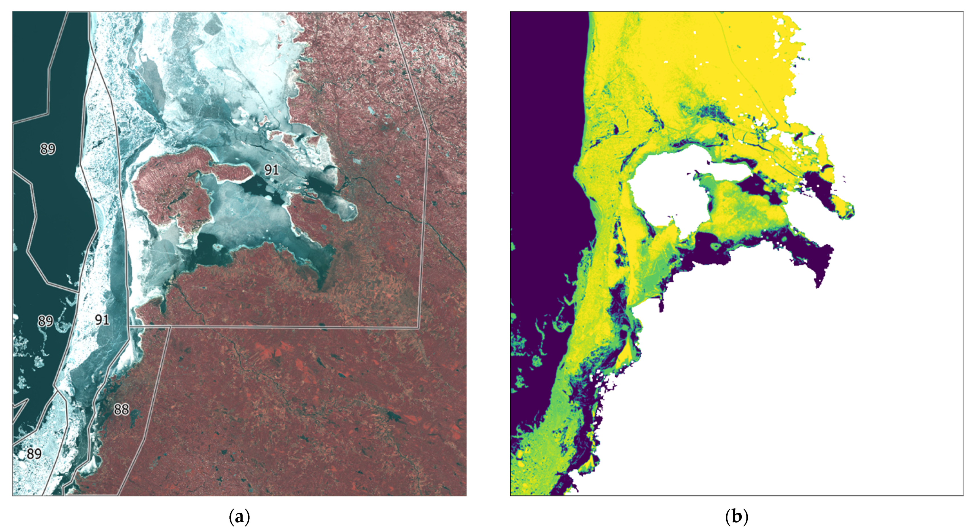
Figure 13 shows a good representation of class 89 from the training polygons. However, class 91, which is not presented in the ice chart, is shown in the classification. Figure 14 shows a dominance of class 91 which is very similar to the training data. Figure 15 shows a classification of Ice Free in the center of the image as well as in the lower part where it looks like there is ice. Since melting usually already starts in April, this is most likely water on top of the ice; this issue needs to be investigated in future studies. Figure 16 shows equivalence in classes 85 and 89. 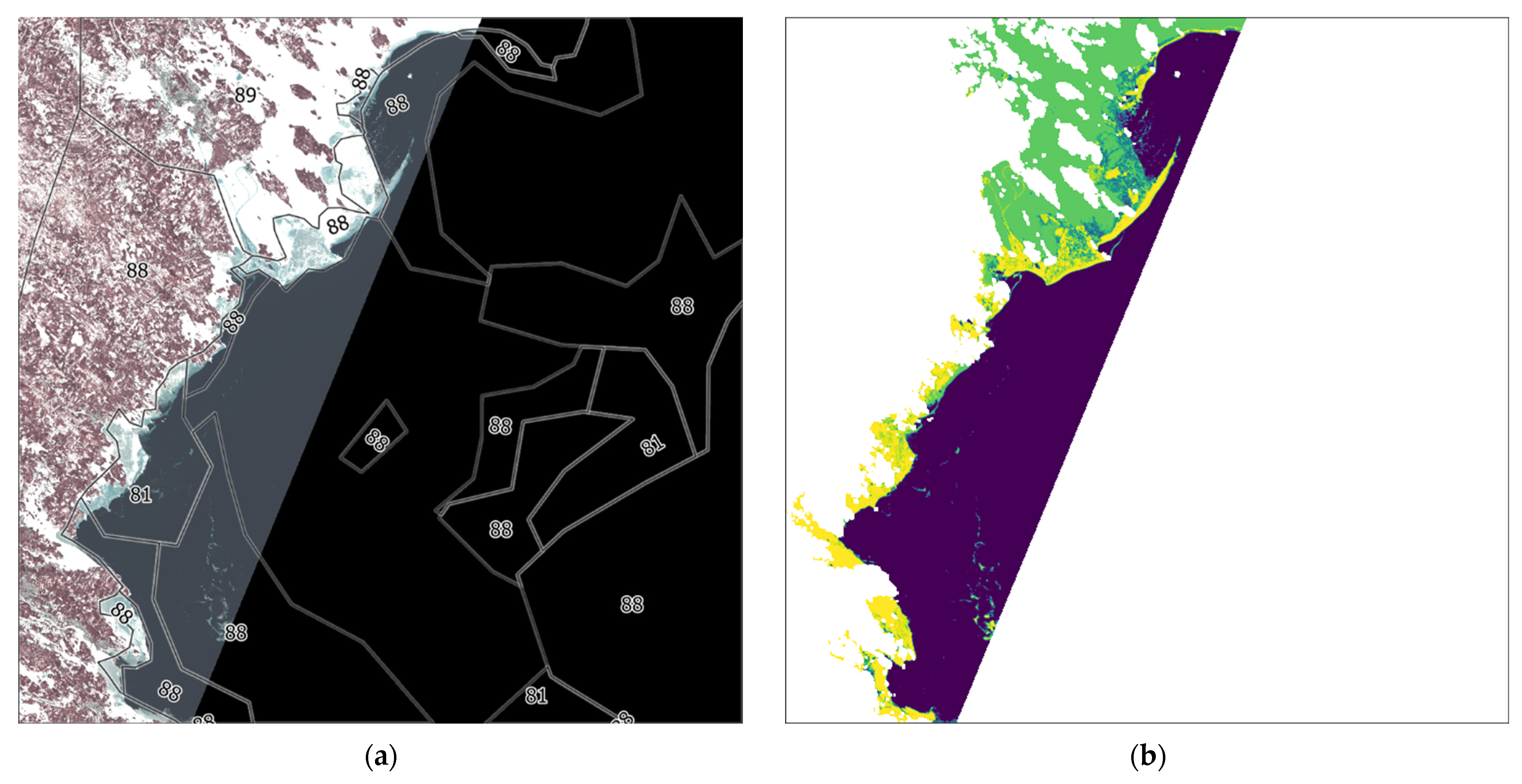Figure 17 shows dominance of class 85, which is very similar to the training data. There is a clear visual discrepancy between near coastal ice (clear white) and the ice further out (darker and partly thinner), but from the classification model, no difference is reported at this time. According to the confusion matrix, the classes 85 and 88 have an accuracy of 50% each. To improve this issue, we recommend including more training data representing these two classes.

It should be noted that the use of the BSH ice charts were of limited use due to the time difference between the acquisition time of the satellite image and the ice chart used for the overlay. The boundaries of the polygons were not accurate enough in respect to the satellite image, which means that the training data did not perfectly match all image areas. The reason for the incoherence of the ice charts provided is that they were not created on the basis of Landsat-8 images itself. Despite these limitations, we used these ice charts because they were a source of training data in digital format for this region. In this study, it can be seen that the model has learned to interpret the classes and make a reliable distinction between ice and water as well as a classification that matches the training data.

When we started our study, we tried to use the whole content image data set of the data cube, thinking that the more data available, the more reliable the results would be. However, this is not necessary if the classification training is done with high quality images, such as the cloud-free images we used. Adding the Ice Free class to the ice classes has greatly improved the results.

Currently, the results do not include all classes that might be represented. By extending the training data, it will be possible to subdivide the results into additional, more sophisticated classes in the future.

The major limitation in using optical imagery is cloud cover. An attempt was made during the study to classify overcast imagery, nevertheless, the embedded cloud mask of the Landsat-8 quality filter is not precise enough to allow a clear distinction. Since the results were not satisfactory, it was decided to perform the study only with cloud-free images. Creating a more realistic cloud mask is an issue for future analysis. In the meantime, the cloud mask provided by Landsat-8 can be used for a usability assessment for value, adding ice classification in an upstream pre-processing step.

The suggested approach is intended to be used in NRT maritime operations. Therefore, the proposed model was designed to provide better performance compared to CNN models, since there was an avoidance of convolutional computation [26].

5. Conclusions

In this study, a neural network for classifying sea ice in the region of the Baltic Sea was deployed. The training data set was generated based on the ice Stage of Development charts provided by the BSH and Landsat-8 satellite imagery. An accuracy of 87.5% was achieved.

The results are promising and show an improvement in the discrimination of sea ice and water compared to the original BSH ice charts. Visual analysis shows that classification and mapping of ice is consistent and enables a significant improvement in the frame of level of detail and discrimination. The use of optical satellite imagery is limited by cloud cover and solar radiation especially in northern regions. However, this study opens the possibility of classifying further satellite imageries in the context of ice services like Sentinel-2 or Sentinel-3 imagery using the same BSH ice charts available for dedicated regions. The results out of the model could also be used to compare the ice charts derived from radar imagery for validation.

For the future, we plan to extend the approach to the images acquired by the new Landsat-9 satellite, which was launched in September 2021, and continue the Landsat mission using the same OLI sensor. The chosen approach can be considered sensor-independent and can therefore be applied to other satellite data, such as Sentinel-2. Data fusion with SAR imagery is also proposed. With regard to the planned extensions, the data cube database offers excellent possibilities, as it can be expanded with these additional products. It is planned for the future that the required ice classification for the requested areas of the Baltic Sea region can be automatically derived directly by using Landsat-8 and Landsat-9 satellite imageries, which are provided for the ice service in Near-Real-Time directly after reception at the DLR ground station Neustrelitz.

References

1. Stephenson, S.R.; Pincus, R. Challenges of Sea-Ice Prediction for Arctic Marine Policy and Planning. J. Borderl. Stud. 2017, 33, 255–272. [Google Scholar] [CrossRef]
2. Goerlandt, F.; Montewka, J.; Zhang, W.; Kujala, P. An Analysis of Ship Escort and Convoy Operations in Ice Conditions. Saf. Sci. 2017, 95, 198–209. [Google Scholar] [CrossRef]
3. Kotovirta, V.; Jalonen, R.; Axell, L.; Riska, K.; Berglund, R. A System for Route Optimization in Ice-Covered Waters. Cold Reg. Sci. Technol. 2009, 55, 52–62. [Google Scholar] [CrossRef]
4. Zakhvatkina, N.; Smirnov, V.; Bychkova, I. Satellite SAR Data-Based Sea Ice Classification: An Overview. Geosciences 2019, 9, 152. [Google Scholar] [CrossRef] [Green Version]
5. Chen, Y.; Lin, Z.; Zhao, X.; Wang, G.; Gu, Y. Deep Learning-Based Classification of Hyperspectral Data. IEEE J. Sel. Top. Appl. Earth Obs. Remote Sens. 2014, 7, 2094–2107. [Google Scholar] [CrossRef]
6. Perovich, D.K. US Army Corps of Engineers, Cold Regions Research & Engineering Laboratory. In The Optical Properties of Sea Ice; National Technical Information Service: Springfield, VA, USA, 1996. [Google Scholar]
7. Richter, R.; Schläpfer, D. Atmospheric and Topographic Correction (ATCOR Theoretical Background Document); DLR—German Aerospace Center: Wessling, Germany, 2021. [Google Scholar]
8. Han, Y.; Liu, Y.; Hong, Z.; Zhang, Y.; Yang, S.; Wang, J. Sea Ice Image Classification Based on Heterogeneous Data Fusion and Deep Learning. Remote Sens. 2021, 13, 592. [Google Scholar] [CrossRef]
9. Atkinson, P.M.; Tatnall, A.R.L. Introduction Neural Networks in Remote Sensing. Int. J. Remote Sens. 1997, 18, 699–709. [Google Scholar] [CrossRef]
10. Park, K.; Kim, D.-H. Accelerating Image Classification Using Feature Map Similarity in Convolutional Neural Networks. Appl. Sci. 2018, 9, 108. [Google Scholar] [CrossRef] [Green Version]
11. Zhang, L.; Zhang, L.; Du, B. Deep Learning for Remote Sensing Data: A Technical Tutorial on the State of the Art. IEEE Geosci. Remote Sens. Mag. 2016, 4, 22–40. [Google Scholar] [CrossRef]
12. Jiang, W.; He, G.; Long, T.; Ni, Y.; Liu, H.; Peng, Y.; Lv, K.; Wang, G. Multilayer Perceptron Neural Network for Surface Water Extraction in Landsat 8 OLI Satellite Images. Remote Sens. 2018, 10, 755. [Google Scholar] [CrossRef] [Green Version]
13. Damerow, H.; Richter, J.; Missling, K.-D. Evolution of DLR’s Multi-Mission Ground Station as a Reception Facility in the Middle of Europe (Sektion 2). Tsilkovski Conf. 2018, 53, 1–11. [Google Scholar]
14. Ihlen, V. Landsat 8 Data Users Handbook; U.S. Geological Survey: Sioux Falls, SD, USA, 2015. [Google Scholar]
15. Killough, B. Overview of the Open Data Cube Initiative. In Proceedings of the IGARSS 2018—2018 IEEE International Geoscience and Remote Sensing Symposium, Valencia, Spain, 22–27 July 2018; pp. 8629–8632. [Google Scholar]
16. Ouaidrari, H.; Vermote, E.F. Operational Atmospheric Correction of Landsat TM Data. Remote Sens. Environ. 1999, 70, 4–15. [Google Scholar] [CrossRef]
17. Brandt, R.E.; Warren, S.G.; Worby, A.P.; Grenfell, T.C. Surface Albedo of the Antarctic Sea-ice Zone. J. Clim. 2005, 18, 3606–3622. [Google Scholar] [CrossRef] [Green Version]
18. Pang, B.; Nijkamp, E.; Wu, Y.N. Deep Learning With TensorFlow: A Review. J. Educ. Behav. Stat. 2020, 45, 227–248. [Google Scholar] [CrossRef]
19. Madhiarasan, M.; Deepa, S.N. Comparative Analysis on Hidden Neurons Estimation in Multi Layer Perceptron Neural Networks for Wind Speed Forecasting. Artif. Intell. Rev. 2017, 48, 449–471. [Google Scholar] [CrossRef]
20. Ruder, S. An Overview of Gradient Descent Optimization Algorithms. arXiv 2017, arXiv:1609.04747. [Google Scholar]
21. Sharma, S.; Sharma, S.; Athaiya, A. Activation Functions in Neural Networks. Data Sci. 2017, 6, 310–316. [Google Scholar] [CrossRef]
22. Ittiyavirah, S.; Jones, S.; Siddarth, P. Analysis of Different Activation Functions Using Backpropagation Neural Networks. J. Theor. Appl. Inf. Technol. 2013, 47, 1344–1348. [Google Scholar]
23. Kingma, D.P.; Ba, J. Adam: A Method for Stochastic Optimization. arXiv 2017, arXiv:1412.6980. [Google Scholar]
24. Agarap, A.F. Deep Learning Using Rectified Linear Units (ReLU). arXiv 2019, arXiv:1803.08375. [Google Scholar]
25. Grandini, M.; Bagli, E.; Visani, G. Metrics for Multi-Class Classification: An Overview. arXiv 2020, arXiv:2008.05756. [Google Scholar]
26. Botalb, A.; Moinuddin, M.; Al-Saggaf, U.M.; Ali, S.S.A. Contrasting Convolutional Neural Network (CNN) with Multi-Layer Perceptron (MLP) for Big Data Analysis. In Proceedings of the 2018 International Conference on Intelligent and Advanced System (ICIAS), Kuala Lumpur, Malaysia, 13–14 August 2018. [Google Scholar] [CrossRef]
Figure 1. Landsat-8 false color image collection over the Baltic Sea at 16 February 2021; BSH Ice Chart for 16 February 2021 (blue polygons) with their ICESOD codes.
Remotesensing 14 01975 g001
Figure 2. Ice classification general flowchart.
Remotesensing 14 01975 g002
Figure 3. Spectral albedos of sea ice, after [17].
Remotesensing 14 01975 g003
Figure 4. (a) Landsat-8, 16 February 2021; (b) Ice mask (blue).
Remotesensing 14 01975 g004
Figure 5. (a) Ice mask overlaid with the BSH Ice Chart for 22 March 2019; (b) Water mask for 22 March 2019.
Remotesensing 14 01975 g005
Figure 6. DNN architecture. The input layer has 5 nodes corresponding to the Landsat-8 top of atmosphere values, the output layer has 5 nodes corresponding to the ICESOD codes. The 4 hidden layers have 40 nodes each.
Remotesensing 14 01975 g006
Figure 7. Loss vs. Epoch. After 21 epochs, the training loss (orange) has a value of 0.3040 and the validation loss (blue) has a value of 0.3041.
Remotesensing 14 01975 g007
Figure 8. Accuracy vs. Epoch. After 21 epochs, the training accuracy (orange) has a value of 0.8751 and the validation accuracy (blue) has a value of 0.8750.
Remotesensing 14 01975 g008
Figure 9. Confusion Matrix.
Remotesensing 14 01975 g009
Figure 10. (a) Landsat-8 false color for 06 March 2019; BSH ice chart for 05 March 2019; (b) ICESOD classification.
Remotesensing 14 01975 g010
Figure 11. (a) Landsat-8 false color for 22 March 2019; BSH ice chart for 21 March 2019; (b) ICESOD classification.
Remotesensing 14 01975 g011
Figure 12. (a) Landsat-8 false color for 22 March 2019; BSH ice chart for 21 March 2019; (b) ICESOD classification.
Remotesensing 14 01975 g012
Figure 13. (a) Landsat-8 false color for 27 March 2019; BSH ice chart for 27 March 2019; (b) ICESOD classification.
Remotesensing 14 01975 g013
Figure 14. (a) Landsat-8 false color for 16 April 2019; BSH ice chart for 15 April 2019; (b) ICESOD classification.
Remotesensing 14 01975 g014
Figure 15. (a) Landsat-8 false color for 23 April 2019; BSH ice chart for 24 April 2019; (b) ICESOD classification.
Remotesensing 14 01975 g015
Figure 16. (a) Landsat-8 false color for 16 February 2021; BSH ice chart for 16 February 2021; (b) ICESOD classification.
Remotesensing 14 01975 g016
Figure 17. (a) Landsat-8 false color for 16 February 2021; BSH ice chart for 16 February 2021; (b) ICESOD classification.
Remotesensing 14 01975 g017