On Turbulent Features of E × B Plasma Motion in the Auroral Topside Ionosphere: Some Results from CSES-01 Satellite

Abstract

The recent Chinese Seismo-Electromagnetic Satellite (CSES-01) provides a good opportunity to investigate some features of plasma properties and its motion in the topside ionosphere. Using simultaneous measurements from the electric field detector and the magnetometers onboard CSES-01, we investigate some properties of the plasma E × B drift velocity for a case study during a crossing of the Southern auroral region in the topside ionosphere. In detail, we analyze the spectral and scaling features of the plasma drift velocity and provide evidence of the turbulent character of the E × B drift. Our results provide an evidence of the occurrence of 2D E × B intermittent convective turbulence for the plasma motion in the topside ionospheric F2 auroral region at scales from tens of meters to tens of kilometers. The intermittent character of the observed turbulence suggests that the macro-scale intermittent structure is isomorphic with a quasi-1D fractal structure, as happens, for example, in the case of a filamentary or thin-tube-like structure. Furthermore, in the analyzed range of scales we found that both magnetohydrodynamic and kinetic processes may affect the plasma dynamics at spatial scales below 2 km. The results are discussed and compared with previous results reported in the literature.

1. Introduction

In the geospace environment, such as the Earth’s ionosphere and magnetosphere, plasma dynamics can display multiscale features and chaos. As it occurs in several space and astrophysical plasmas, the chaotic nature of the plasma dynamics in the geospace environment is due to the occurrence of turbulent processes. This happens, for instance, at high-latitude ionospheric regions, where plasma dynamics was shown to be characterized by turbulence as revealed, for example, by the irregular and chaotic character of the electric and magnetic field fluctuations in the ULF (Ultra Low Frequency) and ELF (Extra Low Frequency) spectral ranges [1,2,3]. In addition, previous studies of the ionospheric electric, magnetic and electron density fluctuations have shown that the fluctuations are characterized by power-law spectral densities, scaling features and non-Gaussian statistics of spatial and temporal increments at small/short scales (see, e.g., [4,5,6,7,8,9] and references therein). In detail, in the auroral regions, it has been found by Kintner et al. [10] that the origin of electric field broadband spectra and the features of its fluctuations are probably caused by the occurrence of intermittent turbulence [10,11], due to the sporadic fast interactions between localized coherent plasma structures [4,12]. In any case, most of the observed fluctuations of fields and plasma parameters in the high-latitude ionospheric regions are characterized by very complex multiscale features that might affect the plasma dynamics [4,13,14].

The high variability of the electric and magnetic field fluctuations can affect the plasma dynamics through the term $\mathbf{E}\times \mathbf{B}$, which can be strongly influenced by the multiscale and turbulent character of the field fluctuations. The plasma $\mathbf{E}\times \mathbf{B}$ drift has been widely investigated in the ionospheric equatorial region, where the variations of the vertical plasma velocity drift play a relevant role in generating ionospheric irregularities [15,16,17,18]. Conversely, it is believed less relevant in the auroral region, especially at the typical altitudes where auroral emission occurs [19]. This is because at this altitude the presence of neutrals can interfere with the $\mathbf{E}\times \mathbf{B}$ drift disrupting the coherent plasma motion perpendicular to the magnetic field direction due to the ion-neutral collisions. This mechanism is at the origin of the well-known Hall current [19]. However, at higher altitudes where the neutrals’ density is lower, the $\mathbf{E}\times \mathbf{B}$ drift may play a relevant role in the dynamics of the plasma also in the auroral regions, and can be relevant to the formation of plasma irregularities.

Recently, the Chinese Seismo-Electromagnetic Satellite (CSES-01) [20,21], launched on February 2018 and equipped with a large set of instruments, including an electric field detector (EFD) [22,23], a flux gate (HPM) and a search-coil (SCM) [24] magnetometer, has had the opportunity to explore the Southern auroral oval region during a time interval characterized by the occurrence of a magnetospheric substorm. During the crossing of the southern auroral region, the satellite has measured simultaneously the magnetic and electric field fluctuations [25]. CSES-01, which has been originally designed to study possible correlations between seismic events and iono/magnetospheric perturbations, flies in the topside F2 ionosphere at ∼500 km of altitude on a Sun-synchronous orbit. Thus, it can also provide the opportunity to explore the plasma dynamics at an altitude higher than that at which the typical auroral phenomena occur. Generally CSES-01 is operative at geographic latitude $\left|Lat\right|<{65}^{\circ }$, and thus the observation of high-latitude phenomena is sporadic and limited to a few periods in which the Earth’s dipole tilt angle is higher than $|{15}^{\circ }|$, corresponding to solstices. On 11 August 2018 from 21:41 UT to 21:45 UT, CSES-01 was in operational mode during a crossing of the Southern polar F2 topside ionosphere. Its measurements allowed us [25] to investigate some interesting features of the electric field fluctuations in the auroral region and to establish the very complex structure of electric field fluctuations probably due to the occurrence of intermittent turbulence [4,12].

This study sits out to investigate the spectral and scaling features of the plasma $\mathbf{E}\times \mathbf{B}$ drift velocity using magnetic and electric field measurements from the HPM, SCM and EFD experiments onboard CSES-01 during the crossing of the Southern auroral region occurred on 11 August 2018. In detail, this case study seeks to examine the multiscale character of the plasma drift velocity $\mathbf{E}\times \mathbf{B}$.

2. Data Description

We consider magnetic and electric field data recorded by HPM, SCM and EFD instruments [22,24] onboard CSES-01 during a crossing of the Southern polar ionosphere on 11 August 2018 from 21:42:30 UT to 21:45:00 UT. During this time interval CSES-01 partially crosses the Southern auroral oval region in its ascending orbit near 02:00 MLT when auroral precipitation is going on. This time interval is, indeed, characterized by a moderate/high auroral substorm activity, as indicated by the value of the auroral electrojet index, AE > 500 nT [25]. This period has already been investigated in previous papers [25,26], to which the reader may refer for more information.

We use magnetic field data with a resolution of 1 sample/s from HPM and with a resolution of 10 k samples/s from SCM and electric field measurements with a resolution of 5000 samples/s. Magnetic field data from HPM and SCM are joined and successively reduced at the same resolution of EFD, i.e., 5000 samples/s, in order to compute the plasma $\mathbf{E}\times \mathbf{B}$ drift velocity, i.e.,

$${\mathbf{v}}_D=\frac{\mathbf{E}\times \mathbf{B}}{B^2},$$

(1)

where $\mathbf{E}$ and $\mathbf{B}$ are the electric and magnetic field, respectively. Data are in the geographic coordinate system, $[x,y,z]$, where the X-component is pointing to the geographic North, the Y-component to East and the Z-component to Earth’s center. Furthermore, the electric field components are corrected subtracting the term ${\mathbf{E}}_s={\mathbf{v}}_s\times \mathbf{B}$, where ${\mathbf{v}}_s$ is the satellite velocity, which is due to the satellite motion in the Earth’s magnetic field. Lastly, the velocity field is downsampled to the resolution of 250 samples/s by averaging the original 5000 samples/s data on consecutive boxes of 20 points. Thus, considering the satellite velocity, which is of the order of $v_s\simeq 8$ km/s, and the chosen resolution of 250 samples/s, we are capable of exploring velocity fluctuations up to scales of the order of ∼30 m. This length scale is well below the ion inertial length scale, which is of the order of $2÷3$ km for $O^{+}$ and $10÷20$ m for $e^{-}$. This means that we are capable of exploring also the sub-ionic scales.

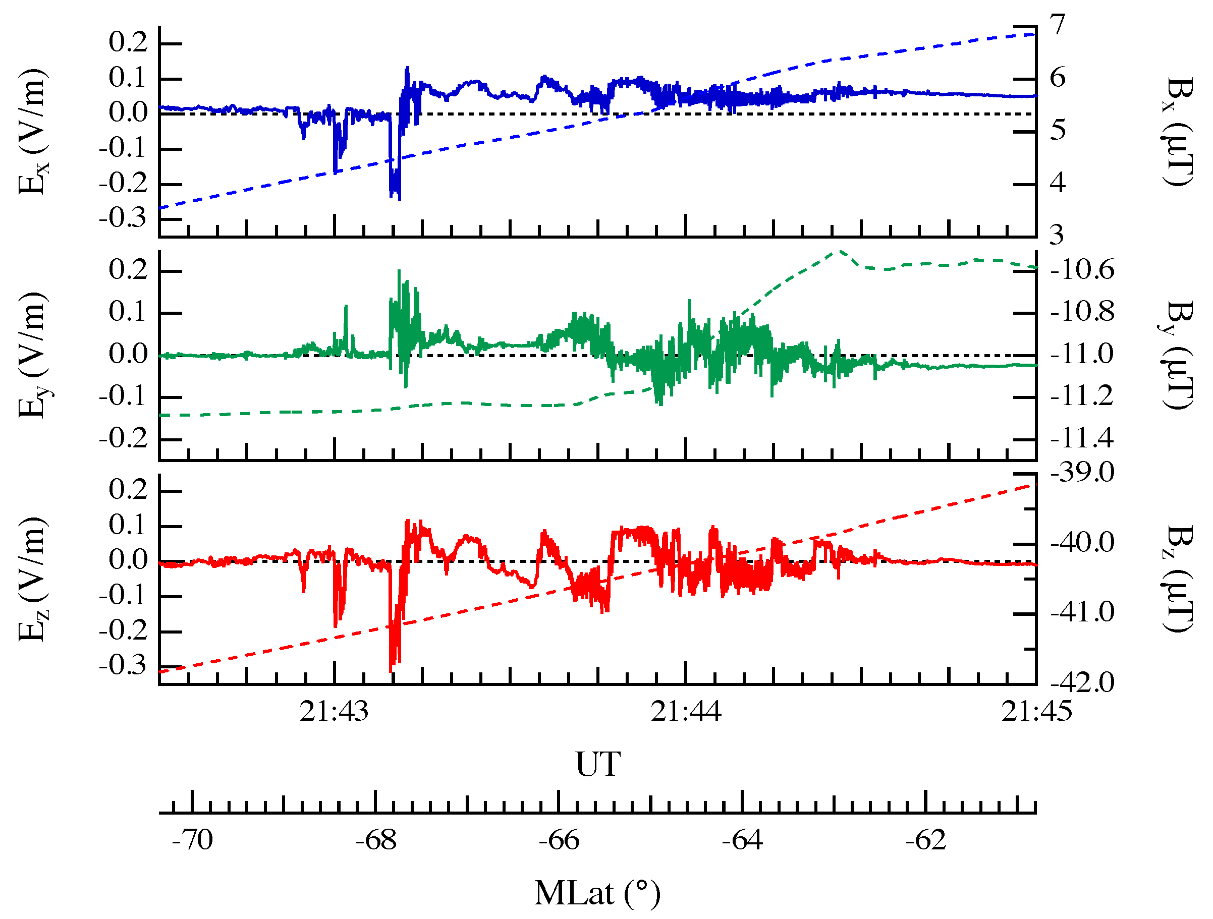
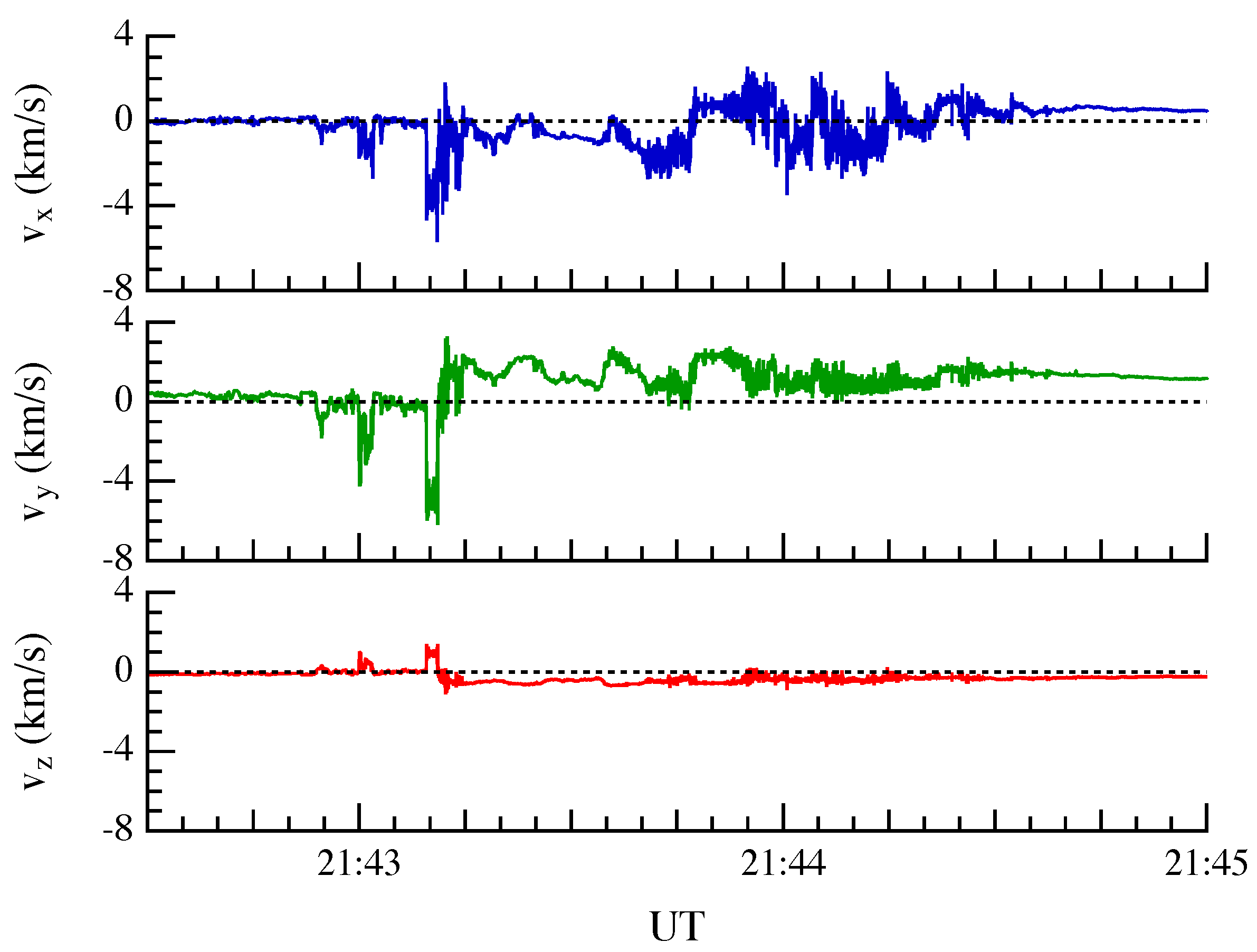
Figure 1 shows the electric and the magnetic field data collected by CSES-01 and used in our analysis. The values of the electric field along the three different directions are similar, ranging between −0.3 V/m and 0.15 V/m. Conversely, the magnetic field is stronger along the z-axis as expected at high latitude being the magnetic field nearly vertical.

Figure 2 reports the plasma drift velocity, ${\mathbf{v}}_D$, computed using Equation (1). Due to the quasi-dipole magnetic field configuration, the velocity field of the plasma in the crossed polar region is mainly horizontal in the $[x,y]$-plane. Although the mean flow direction is along the Y component, the plasma drift velocity shows large fluctuations along the x and y axes, as confirmed by the values of the root mean square along the three axes ${\mathbf{v}}_D^{RMS}\equiv [0.83,1.34,0.35]$ km/s.

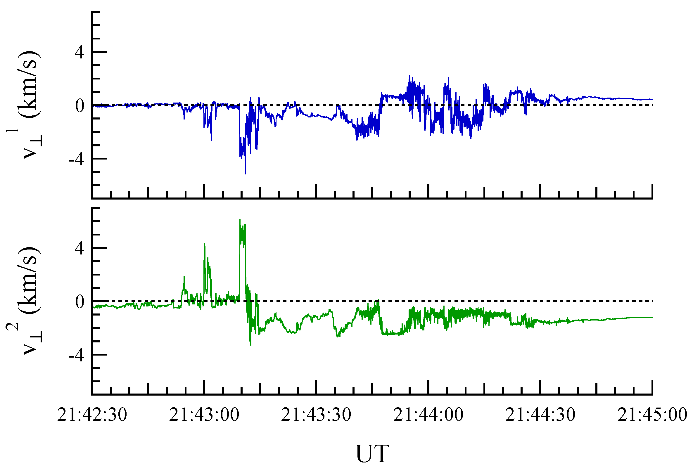
Anyway, the geographic coordinate system is not the optimal reference system for our analysis. Usually, the analysis of the fluctuation field is done in the parallel and perpendicular directions to the magnetic field. For this reason, we change coordinate system and compute the parallel and perpendicular components to the local magnetic field direction of the plasma $\mathbf{E}\times \mathbf{B}$ drift velocity. The component of the drift velocity, which is parallel ($v_{\Vert }$) to the magnetic field direction, is practically zero being $\mid v_{\Vert }/v_{\perp }\mid \ll {10}^{-6}$ (we remark that it is expected to be zero by construction). The two perpendicular components, which describe the horizontal plasma motion, are reported in Figure 3. They are chosen so that $v_{\perp }^{\left(1\right)}$ and $v_{\perp }^{\left(2\right)}$ are almost along the direction of North (x) and East ($-y$) axis, respectively. In detail, for each point we consider the local magnetic field direction (i.e., the geomagnetic field direction that is essentially oriented in the z-direction) and define two unitary vectors in the plane perpendicular to geomagnetic field direction, with components mainly along x- and y-directions. This defines the local reference frame. Successively, we compute the components of the $\mathbf{E}\times \mathbf{B}$ along these two perpendicular unitary vectors.

The effective dimension $d^{*}$ of the drift velocity fluctuation field can be measured by applying the covariance analysis, which allows us to estimate the eigenvalues of the covariance matrix of the drift velocity. Indeed, knowing the eigenvalues of covariance matrix, we can compute the effective dimension, $d^{*}$, of the fluctuating field as

$$d^{*}=\frac{1}{{\lambda }_{max}}\sum _i{\lambda }_i$$

(2)

where ${\lambda }_i$ are the eigenvalues and ${\lambda }_{max}$ is the maximum eigenvalue. In our case, we get an effective dimension $d^{*}\simeq 1.35$. This quantity provides an indication of the dimension of the phase-space spanned by the field fluctuations. In our case, being $1<d^{*}<2$, we expect that the drift velocity fluctuation field can be confined in a 2D space. Consequently, we could assume to deal with a 2D plasma motion. Anyway, we remark that the effective dimension $d^{*}$ is not to be confused with the fractal dimension associated with the plasma dynamics under the drift velocity.

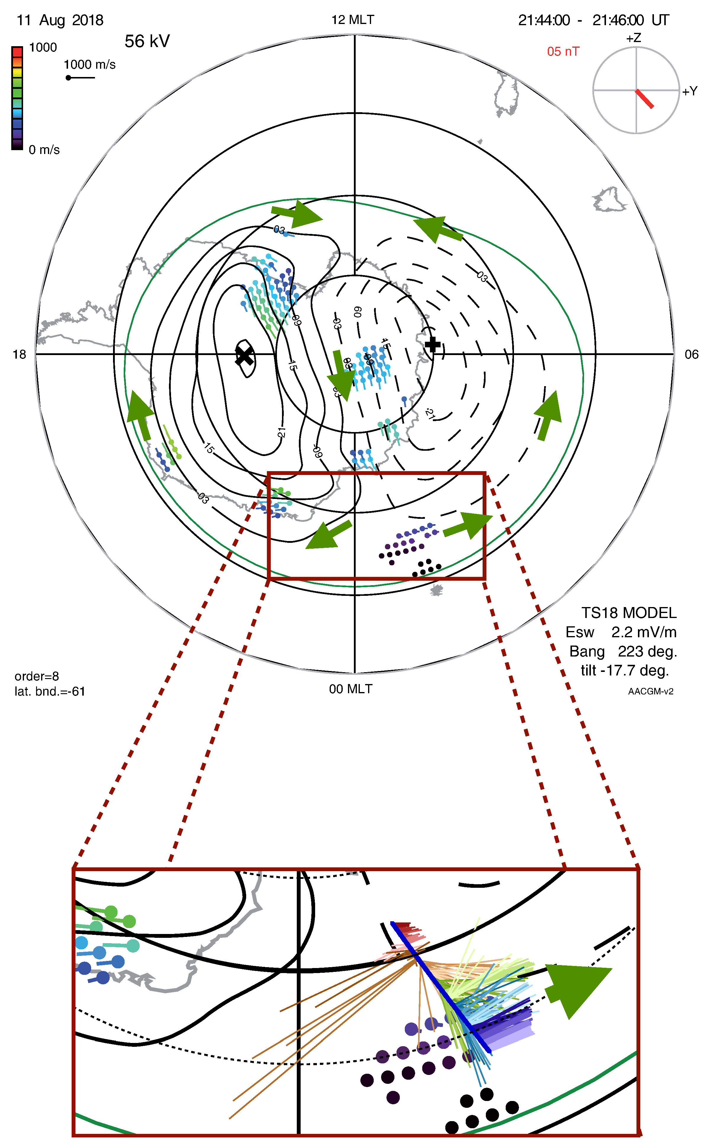
Before proceeding in the analysis, we check the consistency of the obtained average velocity field with the macroscopic overall convection pattern, that can be reconstructed from measurements of the Super Dual Auroral Radar Network (SuperDARN) radars operating in the Southern polar hemisphere. SuperDARN is an international scientific radar network consisting of high frequency (HF) coherent scatter radars that is operated under international cooperation. The SuperDARN data are mainly used to monitor the dynamics of the ionosphere and upper atmosphere in the high- and mid-latitude regions through the production of global plasma convection maps. However, these data can also be used to study many others geospace phenomena including field aligned currents, geomagnetic storms, magnetospheric substorms, magnetic reconnection, and interhemispheric plasma convection asymmetries (see, e.g., [27,28,29] and references therein). Figure 4 reports a comparison between the ionospheric convection map as reconstructed from SuperDARN observations relative to the time interval 21:44-21:46 UT, corresponding to the central part CSES-01 track and the convection drift velocity obtained by $\mathbf{E}\times \mathbf{B}$ from CSES-01 measurements.

Global maps of ionospheric convection can be derived from the SuperDARN data using the technique developed by Ruohoniemi and Baker [30] and Shepherd and Ruohoniemi [31]. In this technique, the SuperDARN line-of-sight velocities are fitted to an expansion of the high-latitude electrostatic potential in spherical harmonic functions. In order to constraint the solution in regions where no SuperDARN data are available, additional data from statistical models are used. The convection map shown in Figure 4 has been computed using the statistical model by Thomas and Shepherd [32] for adding data where SuperDARN data are missing. This statistical model (named TS18) has been derived for the Southern and Northern hemispheres using measurements from all the mid-latitude, high-latitude, and polar radars available in the years from 2010 to 2016. The TS18 is capable of producing climatological patterns of ionospheric convection organized by solar wind, interplanetary magnetic field (IMF), and dipole tilt angle conditions. The TS18 model inputs used for the computation of the map in Figure 4 correspond the average values of IMF clock angle (${223}^{\circ }$), solar wind electric field ($E_{sw}=2.2$ mV/m), and dipole tilt angle ($-17.7^{\circ }$) for the time interval of interest (11 August 2018 from 21:42:30 UT to 21:45:00 UT). In Figure 4, the colored vectors represent the fitted SuperDARN velocity vectors. The convection map has been generated by using the Radar Software Toolkit 4.2 [33]. Lastly, the green arrows are designed to facilitate the reader in locating the direction of the plasma convection motion. On the bottom of the same figure, we report a zoom of the plasma convection pattern, which permits us to identify the CSES-01 trajectory during the analyzed period. The trajectory is the blue line, while the color lines refer to the reconstructed plasma $\mathbf{E}\times \mathbf{B}$ drift velocity (${\mathbf{v}}_D$). The length of the lines is proportional to the intensity of the drift velocity while the color (from red to light violet) indicates the time. An overall agreement between the observed convection pattern (green arrow) and the reconstructed $\mathbf{E}\times \mathbf{B}$ drift velocity (colored lines) is found. This confirms the correct reconstruction of the convective plasma $\mathbf{E}\times \mathbf{B}$ drift velocity by using CSES-01 measurements. The only small discrepancy is observed in correspondence with the higher latitude part of CSES-01 trajectory, where there is a plasma flow reversal. This can be due to a localized vortex structure near the lower latitude boundary of the convection cells not resolved in the SuperDARN convection map.

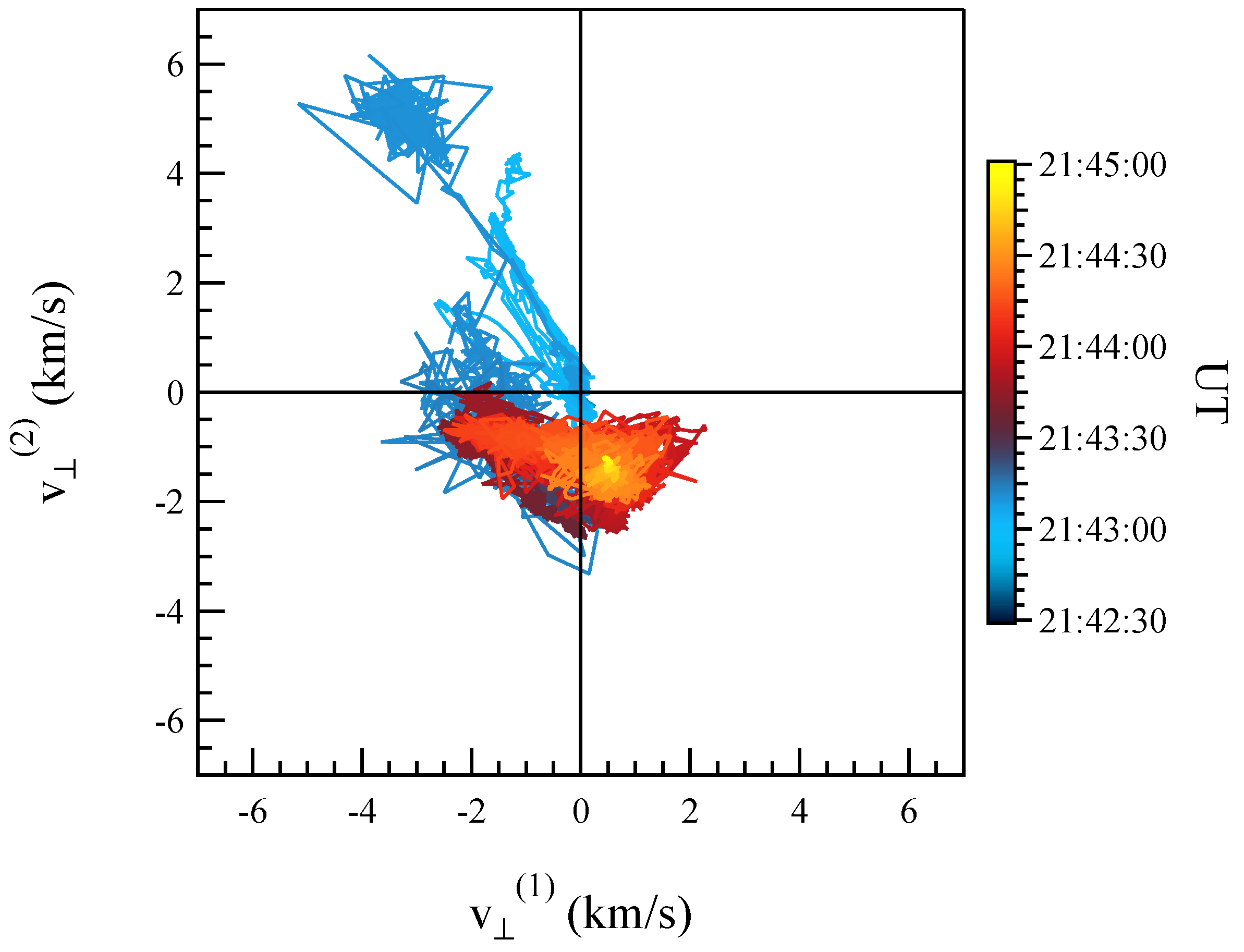
In Figure 5, we report the motion of the velocity vector tip in the plane perpendicular to the magnetic field direction. The motion of the vector tip shows a certain degree of chaoticity, which may be an indication of the occurrence of turbulence in plasma motion.

3. Methods

The analysis of the spectral and scaling features of the plasma $\mathbf{E}\times \mathbf{B}$ drift is done using the standard Fourier power spectral analysis and the structure function analysis applied in fluid and MHD turbulence studies. While the Fourier analysis is a standard method to detect the presence or not of specific modes in the fluctuation field, the structure function analysis, as clearly discussed in Frisch [34], is one of the most powerful methods to investigate scaling features for fully developed turbulence. This approach is, indeed, a powerful method to detect the occurrence anomalous scaling features, i.e., what is generally called intermittency in fluid and MHD turbulence.

In the case of fully developed turbulence, a qth-order structure function, $S^{\left(q\right)}\left(\delta r\right)$, is defined as the qth-order moment of the longitudinal velocity increments, $\delta v_l$, at the spatial scale $\delta r$, i.e.,

$$S^{\left(q\right)}\left(\delta r\right)=\langle {(v_l(r+\delta r)-v_l\left(r\right))}^q\rangle \equiv 〈{\left(\delta v_l\right)}^q〉.$$

(3)

Looking at the definition of Equation (3) for a fixed spatial scale $\delta r$, the qth-order structure function represents the moment of order q of the distribution of the velocity increments at that scale. In the case of a turbulent flow, this quantity is expected to scale in the inertial range according to the following expression,

$$S^{\left(q\right)}\left(\delta r\right)\sim \delta r^{\zeta \left(q\right)},$$

(4)

where the scaling exponents $\zeta \left(q\right)$, as stated by the usual Kolmogorov K41 theory of turbulence, are expected to be $\zeta \left(q\right)=q/3$ [34]. In particular, following the K41 theory and according to the Navier–Stokes equation for an inviscid fluid (i.e., in the limit of an infinite Reynolds number) the third order structure function ($S^{\left(3\right)}\left(\delta r\right)$) is expected to scale with $\zeta \left(3\right)=1$. From the theory, it is possible to write

$$S^{\left(3\right)}\left(\delta r\right)=-\frac{4}{5}ϵ\delta r.$$

(5)

where $ϵ$ is the energy transfer rate along the cascade in the inertial range. Conversely, the $\zeta \left(q\right)=q/3$ dependence of the structure function scaling exponents is essentially a conjecture that implies that a global scale-invariance should exist. However, the observed scaling exponents can show departures from the linear dependence due to intermittency effects. The observed dependence of scaling exponents on the moment order is well described by a convex function of q, so that the global scale invariance is missing. By the way, in the case of intermittency effects, Equation (5) is also expected to hold.

Sometimes, the previous definition of the structure function is generalized considering the absolute value of the velocity differences, $\delta v_l$, i.e.,

$$S^{\left(q\right)}\left(\delta r\right)=〈|\delta v_l{\left(\delta r\right)|}^q〉,$$

(6)

which allows both a better analysis of the dependence of scaling exponents on moment order (see, e.g., [35,36]) and the investigation of non-integer q. We remark that, although structure function analysis is generally defined for increments along the flow direction, it has also been generalized to the case of transverse directions, as well as, for time increments, assuming Taylor’s hypothesis to be valid [37,38].

A simple way to investigate the emergence of intermittency or the validity of the existence of a global scale invariance is to compute the relative scaling of the qth-order structure function on the pth-order one, which is expected to scale as

$$S^{\left(q\right)}\left(\delta r\right)={\left[S^{\left(p\right)}\left(\delta r\right)\right]}^{{\gamma }_p\left(q\right)},$$

(7)

where ${\gamma }_p\left(q\right)=q/p$ in the case of a global scale invariance as the one predicted by K41 theory. We can note how $\gamma \left(q\right)\equiv \zeta \left(q\right)$ if Equation (4) holds and $p=3$ [35,39]. This method has been introduced by Benzi et al. [35] and it is named as extended self-similarity (ESS), which is also valid in the case of low Reynolds number turbulence.

Another interesting quantity is the so-called generalized kurtosis ${\mathsf{\Gamma }}_q\left(\delta r\right)$ [37], which is defined as

$${\mathsf{\Gamma }}_q\left(\delta r\right)\equiv \frac{S^{\left(q\right)}\left(\delta r\right)}{{\left[S^{\left(2\right)}\left(\delta r\right)\right]}^{q/2}}.$$

(8)

It is expected to be constant in the inertial range when global scale invariance holds. Conversely, departures from a constant value are generally referred as the evidence for the occurrence of intermittency. We remark that the emergence of intermittency manifests also in the lack of a scale-invariant shape of the probability density functions (PDFs) of the velocity increments $\delta v\left(\delta r\right)$ with the scale $\delta r$.

We apply the described analysis to the drift velocity field.

4. Results

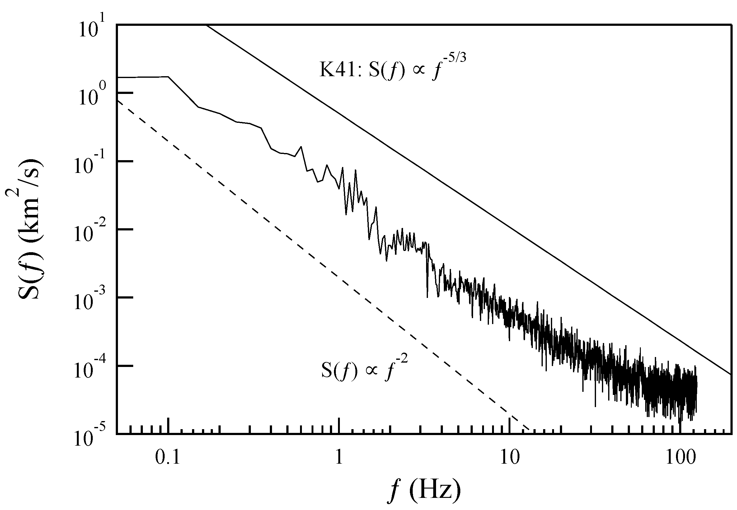
We start our study of the properties of the plasma $\mathbf{E}\times \mathbf{B}$ drift velocity by investigating its spectral features. Figure 6 reports the trace, $S\left(f\right)$, of the power spectral density (PSD) of the components of the drift velocity field, which are perpendicular to the local magnetic field direction. The trace of PSD is defined as the sum of the PSDs of the two perpendicular components. The observed shape of PSD is quite consistent with the spectra expected in the case of two dimensional (2D) $\mathbf{E}\times \mathbf{B}$ convective turbulence in a quasi-steady state [40] or two-dimensional magnetohydrodynamic (MHD) turbulence in absence of Alfvén effect [41]. Indeed, for example, numerical simulations by Gruzinov et al. [40] revealed that when ionospheric plasma density irregularities break up into fingers leading to the formation of stable shear flows, the omnidirectional energy spectrum scaling exponent approaches to $\alpha \simeq -2$ after reaching a quasi-steady state rather than $\alpha \simeq -5/3$ as expected from the K41 theory prediction in the case of isotropic turbulence. In both cases [40,41], the spectral scaling exponents are steeper than the K41 theory prediction, as also occurs in our case being $\alpha \simeq -1.7$. Consistent with the literature, the observed PSD of the components of the plasma drift velocity field seems to support the idea of the occurrence of a strong 2D turbulence in a low$-\beta$ plasma medium [42], where $\beta$, which is the ratio of plasma to magnetic pressure, is a parameter classifying plasma conditions being usually $\beta \ll 1$ for the Earth’s ionospheric plasma.

Let us now move to the analysis of the scaling features by the generalized structure functions, $S^{\left(q\right)}\left(\tau \right)$,

$$S^{\left(q\right)}\left(\tau \right)=\langle |v_i(t+\tau )-v_i\left(t\right){|}^q\rangle ,$$

(9)

where $\tau$ is the timescale, i.e., the time delay used to compute the velocity increments. The analysis is done in the plane perpendicular to the geomagnetic field local direction by considering separately the two components and then averaging the obtained structure functions. The averaging procedure is justified by the fact that the observed scaling features in the two separate perpendicular directions are isotropic, i.e., we do not observe significant differences. The timescale can be associated with a spatial scale $\delta r$ by considering the satellite velocity $v_s$, i.e., $\delta r=\tau v_s$. Here, we investigate the timescale in the range from 4 ms to 3 s, approximately corresponding to a range of spatial scale $\delta r\in [0.03,23.50]$ km. Clearly, this assumption, which is analogous to the Taylor’s hypothesis, is strictly valid if the transit time is faster than the evolution time of the velocity field at the investigated time scale, an assumption that is nearly valid in the low-frequency range, that is, where we can assume that the temporal fluctuations are principally due to Doppler-shifted and stationary spatial variations (see, e.g., [11,25,43] and references therein). We will return on this point in Section 5.

In the case of scale-invariant signals, the generalized q-order structure functions, $S^{\left(q\right)}\left(\tau \right)$, are expected to depend on the scale $\tau$ according to a power law, i.e.,

$$S^{\left(q\right)}\left(\tau \right)\simeq {\tau }^{\gamma \left(q\right)},$$

(10)

where $\gamma \left(q\right)$ are the scaling exponents, which for a signal characterized by a global scale invariance are expected to depend linearly on the moment order q, i.e., $\gamma \left(q\right)=\alpha q$. In particular, the K41 theory of homogeneous turbulence predicts $\gamma \left(q\right)=q/3$.

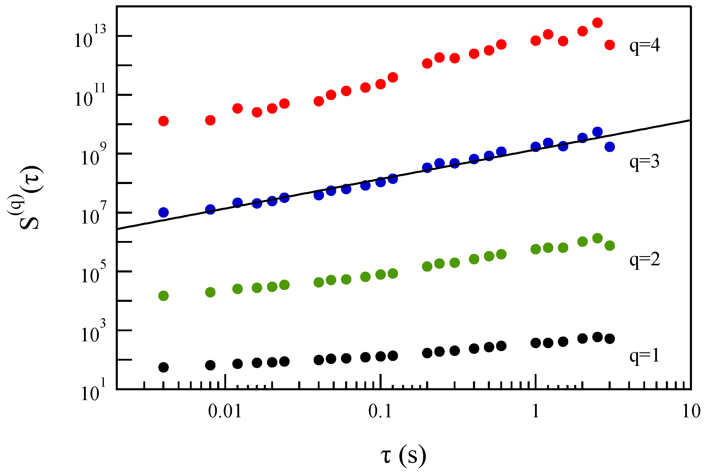
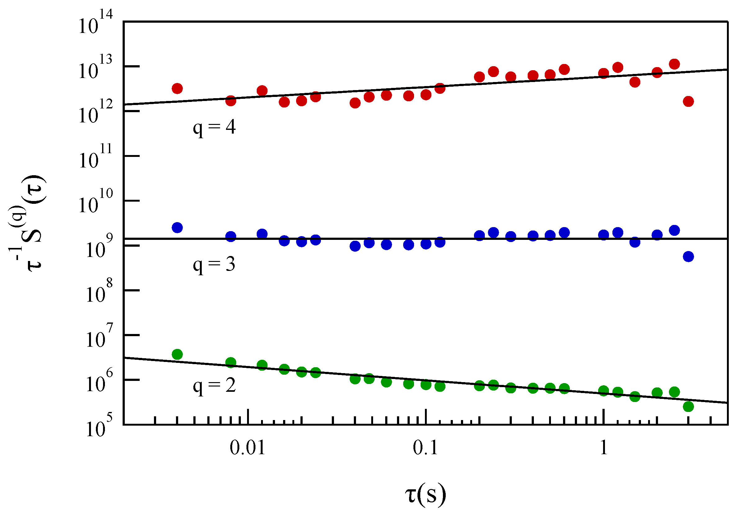
Figure 7 shows the generalized structure functions, $S^{\left(q\right)}\left(\tau \right)$, of the velocity field components perpendicular to the magnetic field direction. Good scaling regimes are observed. In particular, the scaling of the structure functions is observed over near two orders of magnitude from $\tau \sim 0.04$ s to $\tau \sim 4$ s. Furthermore, the third-order structure function, $S^{\left(3\right)}\left(\tau \right)$, displays a range of time scales where a reasonable agreement with the expected linear scaling predicted by the K41 fluid turbulence theory can be found. 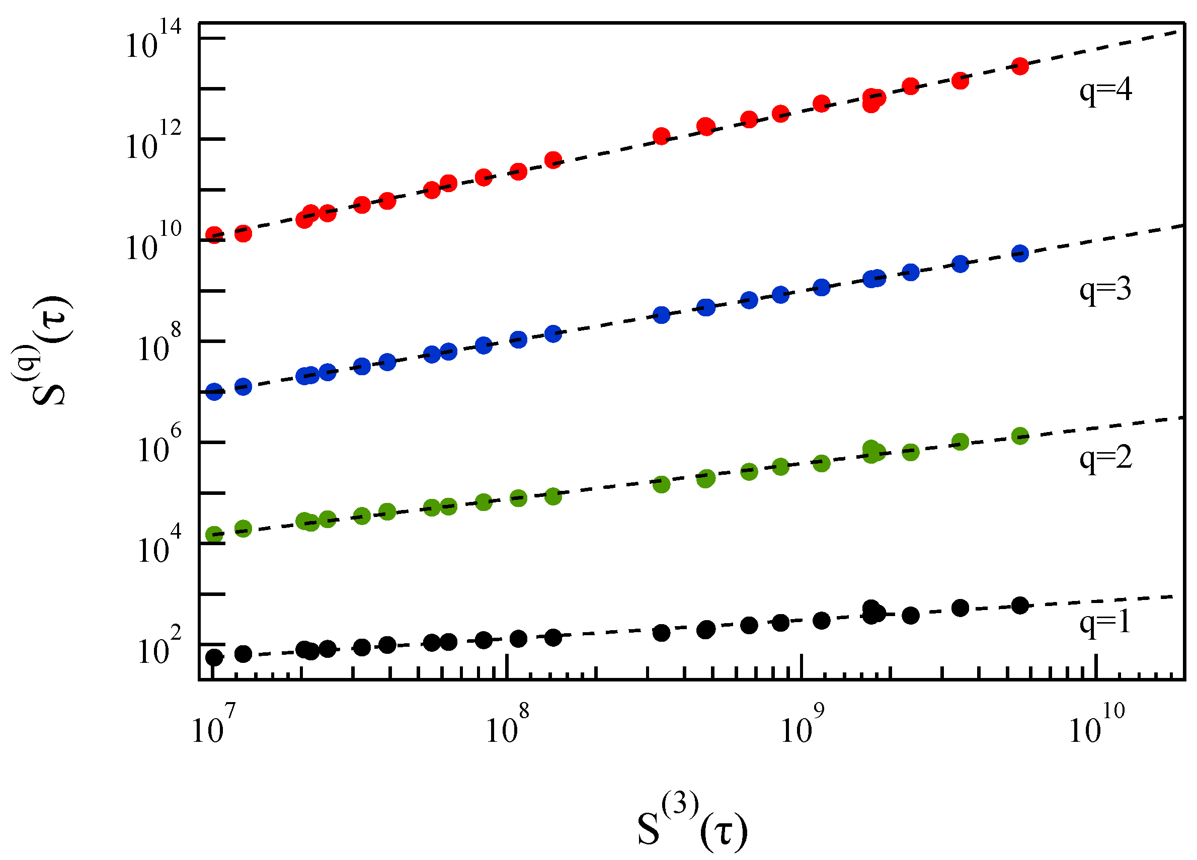This is very clear by plotting the compensated structure functions, ${\tau }^{-1}{S}^{\left(q\right)}\left(\tau \right)$ for $q=2,3$ and 4 as shown in Figure 8. This result suggests that to compute the scaling exponents of the structure functions, we can apply the ESS method introduced by Benzi et al. [35], which is based on the investigation of the relative scaling of the structure functions as reported in Equation (7).

Figure 9 shows relative scaling of the qth-order structure functions, $S^{\left(q\right)}\left(\tau \right)$, on the 3rd-order one for a selected number of moment orders q. For all the moment orders, the qth-order structure functions show a power-law dependence on the corresponding 3rd-order one in agreement with Equation (7). In other terms, ESS is a property of the observed velocity fluctuations perpendicular to the magnetic field direction.

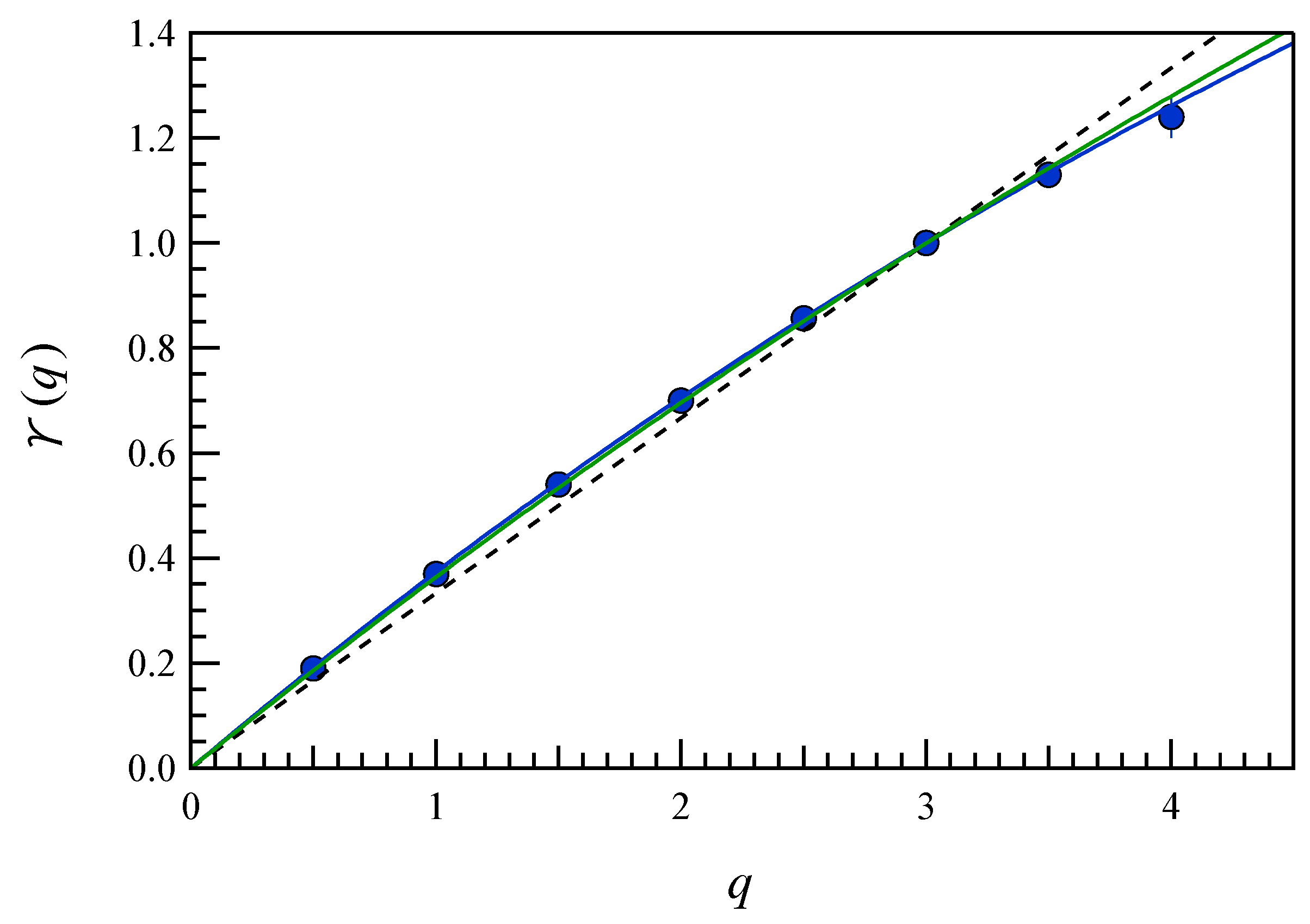
The relative scaling exponents $\gamma \left(q\right)$ are reported as a function of the moment order q in Figure 10. A clear departure on the linear scaling is observed, being the dependence of the scaling exponents on moment order of a convex function. The departure from a linear scaling does not support the occurrence of a global scale-invariance, suggesting instead the emergence of anomalous scaling features, i.e., intermittency.

To characterize and quantify the degree of intermittency, that is how the scaling exponents $\gamma \left(q\right)$ deviate from the Kolmogorov prediction, some intermittency models were proposed, which attempt to explain in particular the anomalous scaling exponents. A model capable of explaining the anomalous scaling exponents is the multifractal model by Meneveau and Sreenivasan [44], known as the P-model. It is a simple model able to describe the energy-cascading process in the inertial range whose scheme is based on the generalized two-scale Cantor set with equal scales, but unequal weights. Thus, we compare the observed trend of the $\gamma \left(q\right)$ exponents with the one predicted by P-model. In detail, we fit the trend of $\gamma \left(q\right)$ as a function of moment order q using the following expression,

$$\gamma \left(q\right)=1-{log}_2\left(p^{\frac{q}{3}}+{(1-p)}^{\frac{q}{3}}\right),$$

(11)

where p is the weight of the measure repartition in the multiplicative process of the two-scale Cantor set. The $P-model$ is an excellent approximation of the observed trend of $\gamma \left(q\right)$ and we get $p=[0.25\pm 0.01]$. Being the value of p significantly different from one-half ($p\ne 0.5$) we may surely assert that the drift velocity fluctuation field has a multifractal structure and that the observed energy repartition at the different scales is an anomalous multiplicative process as the one described by the $P-model$.

In the framework of fluid turbulence, other models have been proposed to explain the convex trend of $\gamma \left(q\right)$. Among these, the She-Leveque (SH) model [45] relates the anomalous scaling with the dimension of the dissipative structure in turbulence. In detail, in the case of fluid turbulence, the SH model predicts for $\gamma \left(q\right)$ the following behavior:

$$\gamma \left(q\right)=\frac{q}{9}+2\left[1-{\left(\frac{2}{3}\right)}^{\frac{q}{3}}\right].$$

(12)

The previous expression, which is specialized for the case of 3D fluid turbulence, was generalized later by Politano and Pouquet [46] (see also ref. Biskamp and Müller [47]). The generalized expression of SH model assumes the following form:

$$\gamma \left(q\right)=(1-x)\frac{q}{3}+C_0\left[1-{\left(1-\frac{x}{C_0}\right)}^{\frac{q}{3}}\right],$$

(13)

where $C_0$ is the co-dimension of the intermittent structures and x is the scaling exponent of the dynamic timescale associated with the most intermittent structure (see [46,47]). Thus, in the case of 3D fluid turbulence, one gets $C_0=2$ and $x=2/3$.

The SH-model (see Equation (13)) can be also written as,

$$\gamma \left(q\right)=\left(1-\frac{C_0}{3}\right)\frac{q}{3}+C_0\left(1-{\beta }^{\frac{q}{3}}\right)$$

(14)

where $\beta =1-x/C_0$ is a parameter related to the degree of intermittency. Indeed, for $\beta \to 1$, there is no intermittency, while if $\beta \le 1$, intermittency is present. In our case, we get $\beta \simeq 2/3$.

Table 1. Observed scaling exponents $\gamma \left(q\right)$ and comparison with results from models and literature.

q	This Work	From Ref. [48]	From Ref. [49]	From Ref. [50]	She-Leveque [45]
1	$[0.37\pm 0.01]$	$[0.37\pm 0.01]$	0.36	0.42	$0.364$
2	$[0.70\pm 0.01]$	$[0.70\pm 0.01]$	0.70	0.75	$0.696$
3	1	$[1.00\pm 0.01]$	1	1	1
4	$[1.24\pm 0.02]$	$[1.28\pm 0.02]$	1.27	1.18	$1.28$

Data from Ref. [50] refer to scaling exponents of Elsässer variables.

shows the values for the first 4 scaling exponents in comparison with Ruiz-Chavarria et al. [48] results from fluid turbulence, with Benzi et al. [49] for 3D convective turbulence, Biskamp and Schwarz [50] simulations on 2D MHD turbulence (in this case data refer to Elsässer variables), and SH 3D fluid model. The observed values are very well in agreement in spite of the different physical scenarios, i.e., $\mathbf{E}\times \mathbf{B}$ convective 2D plasma motion, 3D fluid turbulence [48], 2D MHD simulations [50] and theoretical models [45]. A very good agreement is found with exponents from fluid and convective turbulence. In particular, the good agreement with the SH model [45] suggests that the co-dimension of the intermittent structures is $C_0\simeq 2$.

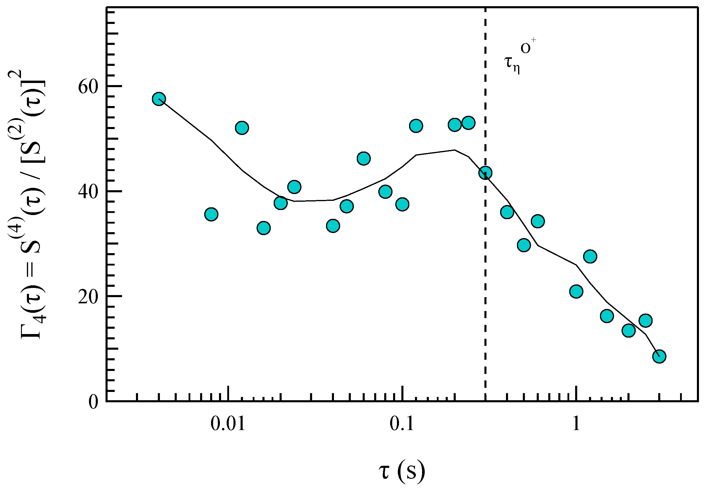
Figure 11 reports the generalized kurtosis ${\mathsf{\Gamma }}_4\left(\tau \right)$ as a function of the timescale $\tau$. ${\mathsf{\Gamma }}_4$ is greater than 3 for all the considered timescales and exhibits an increasing trend for decreasing values of $\tau$. These features provide a strong indication of the non-Gaussian character of the velocity increments (being ${\mathsf{\Gamma }}_4>3$) that is related to the occurrence of intermittency. Another interesting feature of the trend of ${\mathsf{\Gamma }}_4$ is the presence of a local maximum at $\tau \simeq 0.2$ s. This timescale is near the one corresponding to the O${}^{+}$ ion inertial length, $\eta$, assuming a density $n_{{\mathrm{O}}^{+}}\in [1,2]·{10}^5$ cm${}^{-3}$ (this range of values for the oxygen ion density $n_{{\mathrm{O}}^{+}}$ is estimated from electron density $n_{e^{-}}$ [51] assuming quasi-neutrality and that oxygen ions are the more relevant ions at CSES-01 altitude). Indeed, if we consider the Taylor’s hypothesis valid, we have ${\tau }_{\eta }^{O^{+}}=\eta /v_s\simeq 0.3$ s being $v_s\sim 7.8$ km/s the satellite speed.

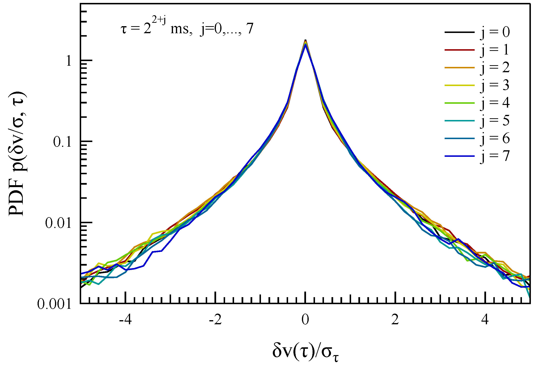
We compute the probability density functions (PDFs) of the velocity increments in the time scale interval from 4 ms to ∼0.5 s. Figure 12 shows the evolution of the standard deviation normalized PDF with the timescale. PDF collapsing does not occur since the shape of the PDFs evolves across different timescale $\tau$, supporting the emergence of intermittency in the velocity field.

We remark that the PDFs are not Gaussian being, indeed, characterized by a leptokurtic shape, which can be well fitted by the following function:

$$p\left(x\right)=\frac{N_0}{{\left[1+\frac{1}{\kappa }{\left(\frac{x}{x_0}\right)}^2\right]}^{\kappa }}exp\left(-\left|\frac{x}{x_c}\right|\right),$$

(15)

where $x=\delta v\left(\tau \right)/{\sigma }_{\tau }$, $x_0$ and $x_c$ are characteristic scales, $N_0$ is a normalization factor and $\kappa$ is the exponent governing the tail behavior. In the case of the smallest-scale PDF at $\tau =4$ ms we get $x_0=[0.130\pm 0.003]$, $x_c=[2.06\pm 0.03]$ and $\kappa =[0.6\pm 0.1]$.

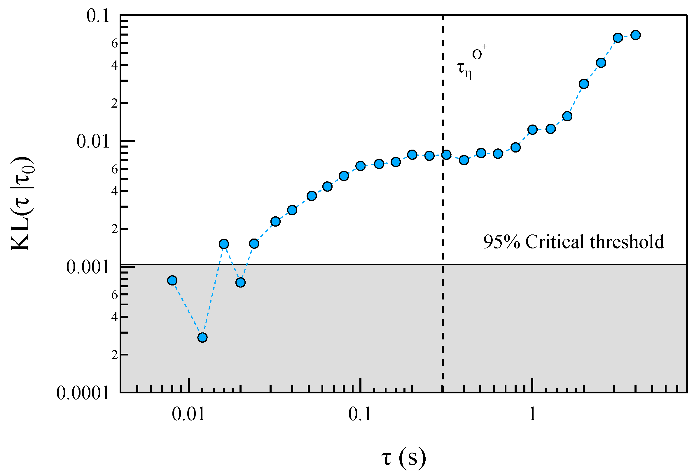
To better characterize the evolution of the PDFs as a function of the timescale, we estimate the Kullback–Leibler ($KL$) distance between the PDFs. In detail, we compute the following quantity:

$$KL(\tau \mid {\tau }_0)={\int }_{-5}^{+5}p(x,\tau ){log}_2\frac{p(x,\tau )}{p(x,{\tau }_0)}dx$$

(16)

where $x=\delta v/\sigma$ and $\tau$ and ${\tau }_0$ are the timescales of the two considered PDFs. Here, we set ${\tau }_0=4$ ms, i.e., the minimum available timescale.

To quantify the significance of the measured $KL$-distance we compute a critical threshold via Monte Carlo simulation. In detail, we generate a series of 1000 random samples $x_i$ containing the same number of values of the actual time series and following the PDF $p(x,{\tau }_0)$ of Equation (15). Successively, we compute the reciprocal $KL$-distance between the distributions of this set of 1000 random samples and evaluate the cumulative distribution of the values of $KL$-distance. The value corresponding to the 95% level of the cumulative distribution of the $KL$-distance is set as the critical threshold to discriminate the significance of the measured $KL$-distance. This threshold value is $K{L}^{*}=1\times {10}^{-3}$.

Figure 13 shows a clear increasing of $KL$-distance with the time scale well above the 95% significance threshold, which is the evidence for the absence of PDF-collapsing. In other words, the PDFs evolve with the timescale of increments so that there is not an invariant shape of the PDFs. This is another counterpart of the absence of a global scale-invariance of increments at different timescales, i.e., of the emergence of intermittency. Furthermore, we observe a short intermediate range of timescales from 0.1 s to 0.6 s where there is a plateau in $KL$ distance. This plateau is well in agreement with the range of timescales ${\tau }_{\eta }^{O^{+}}$ associated with the $O^{+}$ inertial length $\eta$.

5. Discussion

In this study we provided a first analysis of the scaling features of plasma $\mathbf{E}\times \mathbf{B}$ drift velocity in the auroral regions using data collected by the CSES-01 for a case study during a crossing of the Southern polar ionosphere. In detail, our study investigates the drift velocity fluctuations in a range of timescales $\tau \in [0.004,3]$ s, approximately corresponding to a range of spatial scale $\delta r\in [0.03,23.50]$ km, assuming that Taylor’s hypothesis is valid.

The reconstructed 3D convective velocity field is anisotropic, the vertical velocity being very small. This is due to the geomagnetic field configuration in the polar regions, which is mainly vertical. We found a general good consistency of the reconstructed convective velocity field and the overall large scale plasma convection as observed by SuperDARN observations.

Regarding the spectral features, we found evidence of the anisotropic character of the fluctuation field and of the existence of a large interval of frequencies (wave-numbers via Taylor’s hypothesis) where the spectral features follow a power law. The observed spectral exponent of the PSDs in the plane perpendicular to the main geomagnetic field is well in agreement with that expected in the case of 2D $\mathbf{E}\times \mathbf{B}$ convective turbulence ($\left|\alpha \right|\lesssim 2$) in a quasi-steady state [40]. Furthermore, the observed spectral features are also in agreement with the occurrence of 2D MHD turbulence and in strong low-$\beta$ 2D plasma turbulence. Indeed, low-$\beta$ plasma, due to the strong mean magnetic field the plasma motion, is mainly confined in the perpendicular plane, so that the turbulence is essentially 2D. The presence of a strong mean field prevents the bending of magnetic field lines in the mean field direction [50]. Similar spectral features have been found by Kelley and Kintner [52] and Cerisier et al. [53] in the high-latitude ionosphere for the electric field fluctuations, which are strongly correlated to the $\mathbf{E}\times \mathbf{B}$ velocity in that region, and in inertial range of strong turbulence in low-$\beta$ plasmas [42].

We remark that the previous considerations on the spectral properties are based on the assumption of the validity of the Taylor’s hypothesis, which is assumed to be true in the investigated frequency range. Indeed, according to Tchen et al. [42], the conversion of Eulerian observations into Lagrangian ones using the Taylor’s hypothesis is strictly valid only if the flow velocity is very high, or in the case of frozen turbulence, i.e., in the lack of a nonlinear dispersion relation. In other words, the assumption of a linear relationship between f and k is restricted to those cases in which the plasma drift velocity is very high or, if this is not the case, for large wave numbers, as it occurs in the inertial range.

From a general point of view, a difference between 3D and 2D MHD turbulence is the occurrence of an inverse magnetic helicity cascade, which is capable of generating self-organization, i.e., large-scale coherent structures [41]. This scenario seems to be very well in agreement with the occurrence of large scale plasma motion, which manifests in the formation of the two macroscopic convection cells observed in the polar ionosphere (see Figure 4 top panel). The convective motion is clearly forced by the magnetic reconnection phenomenon at the magnetopause, which enhances the plasma convection in the magnetosphere–ionosphere system. In other words, it seems that the nature of the observed turbulence could be isomorphic to a forced convective turbulence.

The analysis of the scaling features of the velocity field increments evidences the occurrence of anomalous scaling properties, supporting the intermittent character of the velocity fluctuation field. The emergence of intermittency is also supported by generalized kurtosis ${\mathsf{\Gamma }}_4$, which shows an increasing trend for decreasing timescale $\tau$, and by the absence of collapsing of the PDFs of the velocity increments at different timescales as shown in Figure 12 and by the evolution of $KL$-distance with the timescales, as shown in Figure 13.

In spite of the different character of the observed turbulence with respect to the ordinary 3D fluid turbulence, the observed anomalous scaling properties are consistent with what is found in the case of the 3D fluid turbulence [48] and theoretical derivations [44,45]. This is a very interesting result that requires a deeper theoretical investigation, but that in any case seems to support the similarity of 2D and 3D plasma turbulence [41], although we have to remark that in the case of 2D MHD turbulence, a more intermittent character is expected with respect to 3D MHD turbulence [50]. Furthermore, the comparison with SH model suggests that the co-dimension of the intermittent structures is $C_0\simeq 2$ and $\beta \simeq 2/3$.

Being $C_0\simeq 2$, in a first approximation considering the case of a 3D system, the fractal dimension of the intermittent structures is $d_F=D-C_0=1$ (where $D=3$ is the system dimension), which suggests that the macro-scale structure is isomorphic with a quasi-1D fractal structure, i.e., a flux tube or a line. This is quite well in agreement with what can be observed in Figure 4 when the satellite enters in the convection region, where the structure of the $\mathbf{E}\times \mathbf{B}$ drift velocity resembles a quasi-cylindrical configuration, i.e., a structure of co-dimension $C_0=2$ and a dimension 1.

Another interesting result from our analysis stands in the behavior of the generalized kurtosis ${\mathsf{\Gamma }}_4$ and the $KL$-distance as a function of timescale $\tau$. As expected from the occurrence of intermittency and anomalous scaling properties we observe an increase of the generalized kurtosis ${\mathsf{\Gamma }}_4$ for decreasing timescales and a departure of the shape of the PDFs from the one at the smallest investigated timescale ${\tau }_0=4$ ms. However, around the typical timescale associated with the oxygen inertial length we observe a maximum in the generalized kurtosis ${\mathsf{\Gamma }}_4$ and a plateau in the increasing trend of the $KL$-distance. This result suggests that in the investigated range of scales, the turbulence associated with $\mathbf{E}\times \mathbf{B}$ convective motion could be more complex than the standard single fluid 2D MHD turbulence. In other words, the multi-ion character of ionospheric plasma could manifest in contiguous multiple regimes of different physical processes, both MHD and kinetic, in the range of timescales from $\tau =5$ ms to $\tau =1$ s [13,14].

6. Summary and Conclusions

In this work, we have investigated the scaling features of the $\mathbf{E}\times \mathbf{B}$ drift motion in the topside F2 polar ionosphere for a case study relative to a crossing of the Southern auroral region by the Chinese Seismo-Electromagnetic satellite (CSES-01) during a geomagnetically disturbed period.

We have found a clear evidence for the occurrence of a turbulent character of the $\mathbf{E}\times \mathbf{B}$ drift velocity in the analyzed region. The observed turbulence seems to be isomorphic to the 2D $\mathbf{E}\times \mathbf{B}$ convective turbulence [40]. Furthermore, the drift velocity fluctuations display an intermittent character as evidenced by the scaling analysis and the behavior of the generalized kurtosis ${\mathsf{\Gamma }}_4\left(\tau \right)$. The observed intermittency features of the $\mathbf{E}\times \mathbf{B}$ drift velocity suggests the hypothesis that intermittency can be related to a macro-scale structure, which is consistent with a quasi-1D fractal structure (thin-flux-like or filamentary structures).

Another interesting result is the emergence of the occurrence of both MHD and kinetic processes in the range of investigated timescales, which can affect the dynamics of the plasma motion at the smallest spatial scales, i.e., below 2 km. This is clearly shown by the trend of the generalized kurtosis ${\mathsf{\Gamma }}_4$ and the Kulback–Leibler distance, which show some deviations from the general trend at a scale consistent with the O${}^{+}$ inertial length. Our findings support the view of very complex dynamics and the idea that it is necessary to consider the multi-species character of the ionospheric plasma medium in order to properly understand and correctly model the small scale ionospheric dynamics, not being sufficient the use of a single fluid theory as is the MHD theory [13,14].

Clearly, further research is required to disentangle and characterize the features of the MHD and kinetic processes involved at the smallest spatial scales. A better comprehension of the observed turbulence processes may benefit from the use of very high-resolution measurements such as those available from the future NanoMagSat mission [54].