Article

Simulative Evaluation of the Underwater Geodetic Network Configuration on Kinematic Positioning Performance

1
School of Earth Sciences and Engineering, Hohai University, Nanjing 211100, China
2
First Institute of Oceanography, Ministry of Natural Resources, Qingdao 266061, China
3
Key Laboratory of Oceanic Surveying and Mapping, Ministry of Natural Resources, Qingdao 266061, China
4
College of Underwater Acoustic Engineering, Harbin Engineering University, Harbin 150001, China
*
Author to whom correspondence should be addressed.
Remote Sens. 2022, 14(8), 1939; https://doi.org/10.3390/rs14081939
Submission received: 21 February 2022 / Revised: 11 April 2022 / Accepted: 12 April 2022 / Published: 17 April 2022
(This article belongs to the Special Issue Remote Sensing Technology for New Ocean and Seafloor Monitoring)

Abstract

:
The construction of underwater geodetic networks (UGN) is crucial in marine geodesy. To provide high-precision kinematic positioning for underwater submersibles, an underwater acoustic geodetic network configuration of three seafloor base stations, one subsurface buoy, and one sea surface buoy is proposed. The simulation results show that, for a 3 km-deep sea, based on the proposed UGN, the submersible positioning range and positioning accuracy are primarily affected by the size of the seafloor base station array, while the height of the subsurface buoy has a greater impact on the submersible positioning accuracy than the positioning range. Considering current acoustic ranging technology, the kinematic positioning performance of the UGN is optimal when the seafloor base stations are 9~13 km apart and the subsurface buoy is less than 2.5 km above the seafloor, which can achieve a submersible positioning accuracy of less than 30 m within an underwater space of 25 km × 25 km × 3 km. The proposed cost-effective UGN configuration can provide high-precision submersible kinematic positioning performance for seafloor surveying and ocean precision engineering. The impact of the underwater environment on the acoustic transmission characteristics should be further investigated.

Graphical Abstract

1. Introduction

Underwater geodetic networks (UGNs) are pivotal for ocean resources exploration, environmental monitoring, and underwater navigation [1]. Due to the attenuation of the electromagnetic field in water, the global navigation satellite system (GNSS) is unsuitable for underwater scenarios [2,3]. Based on the combination of GNSS and acoustic ranging technology (GNSS-A), acoustic underwater geodetic networks can accurately obtain seafloor displacement information [4,5,6,7,8,9]. Moreover, geodetic networks can provide location information for underwater targets, including autonomous underwater vehicles (AUV), remotely operated underwater vehicles (ROV), underwater gliders, underwater buoys, etc., which can be deployed in seafloor surveying and ocean precision engineering [2,3,10,11]. Therefore, the construction of UGNs is currently an important research topic in marine geodesy.
Acoustic positioning systems, such as Long Baseline (LBL) and Ultra-Short Baseline (USBL), are commonly used for underwater positioning [12]. The seafloor beacon array of LBL can be considered a simple underwater geodetic network. With the appropriate sonar and acoustic ranging technology, the positioning range of UGN can reach 10 km with the same ranging precision at a certain depth [13,14]. However, the topography of the seabed could obstruct the bending acoustic signal ray and limit the positioning performance of the geodetic network in seafloor surveying and ocean precision engineering. In general, the longer the required acoustic ranging distance, the higher the seafloor base station’s erection height should be. For the same erection height, the larger the seabed slope, the shorter the acoustic ranging distance becomes [15]. Similar to UGN, Alcocer et al. [16] established a GPS intelligent buoy (GIB) using a sea surface GPS buoy, which can also provide positioning for underwater targets. Techy et al. [10] developed an LBL system with float devices on the water’s surface, which was utilized for underwater glider positioning. In addition, researchers have studied the combined configuration of acoustic positioning systems. The Scripps Institution of Oceanography (SIO) kept the ship in the horizontal center of three seafloor acoustic transponder arrays and performed GPS-A observations [6,7]. To compensate for acoustic ray bending, the SIO also proposed a configuration in that one end of an acoustic interrogator floated tens of meters above the seafloor [17]. Blum et al. [18] added a seafloor-mooring acoustic beacon to the underwater positioning network, whose position was determined by responding acoustic signals to the four seafloor base stations. In addition to acoustic ray bending, the acoustic transmission characteristics, including the multipath effect caused by the acoustic signal reflected from the seabed or the sea surface [19], the Doppler effect caused by the motion of the acoustic source [20,21], the transmission loss of acoustic energy, etc., also affect the acoustic signal propagation.
The construction of an UGN also comprises the maintenance of underwater geodetic stations. To obtain the position of the underwater stations, GNSS-A measurements are primarily performed using sea surface vessels, which restricts the revisit observation frequency due to the high costs and low mobility [22]. To address these shortcomings, alternative observation platforms have been investigated. Imano et al. [23], Tadokoro et al. [21], and Kido et al. [22] conducted GNSS-A measurements using a moored buoy and an autonomous surface vehicle (ASV). Some researchers also investigated the capability of wave gliders and unmanned aerial vehicles (UAVs) as platforms for GNSS-A measurements [11,24,25]. However, the geometric structures formed by the platforms and the station network affect the positioning accuracy. Zhao et al. [26] searched for the lowest geometric dilution of precision (GDOP) and discovered that the circular track can obtain the highest positioning accuracy. Chen et al. [27] also confirmed the optimal circular track in a shallow sea environment. Nakamura et al. [28] comprehensively considered the effects of varying the seafloor transponder array size and the survey line radius on the positioning accuracy and required observation time. The positioning of the underwater stations is subject to the complex ocean environment, and the spatiotemporally varying oceanic physical phenomena, such as the variable sound speed, ocean currents, internal waves, etc., are investigated in positioning [9,29,30]. An underwater positioning with system time synchronization and speed uncertainties has also been studied [31].
To construct an UGN, the network configuration and dimensions should be designed appropriately. One possible configuration is to combine various types of acoustic platforms, including seafloor base stations, underwater moored buoys, and sea surface platforms. However, the impact of the floating height of the underwater acoustic equipment on the positioning performance of combined UGNs has not been investigated. In addition, the network dimension is closely related to the separation of seafloor base stations. The impact of changing network dimensions on the positioning performance of an UGN also needs thorough investigation.
In this study, we propose an underwater geodetic network that combines three seafloor base stations, one underwater subsurface moored buoy, and a sea surface buoy (“3+1+1” configuration). The main purpose of the proposed UGN is to provide kinematic positioning for underwater submersibles applications. To further optimize the UGN, we evaluated the kinematic positioning range and accuracy of the network by simulation tests. By analyzing the separation of the seafloor base stations and the height of subsurface buoys, we evaluated the impact of the network dimensions on the positioning performance. Compared with the network configurations of fewer or more stations, the proposed “3+1+1” configuration with the underwater subsurface moored buoy and the surface buoy improved the kinematic positioning performance and cost-efficiency of the UGN. Additionally, the impact of the acoustic transmission characteristics, e.g., acoustic ray bending, multipath effect, transmission loss, etc., on the acoustic signal propagation of UGN was investigated.

2. Methods

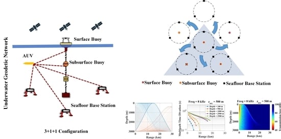
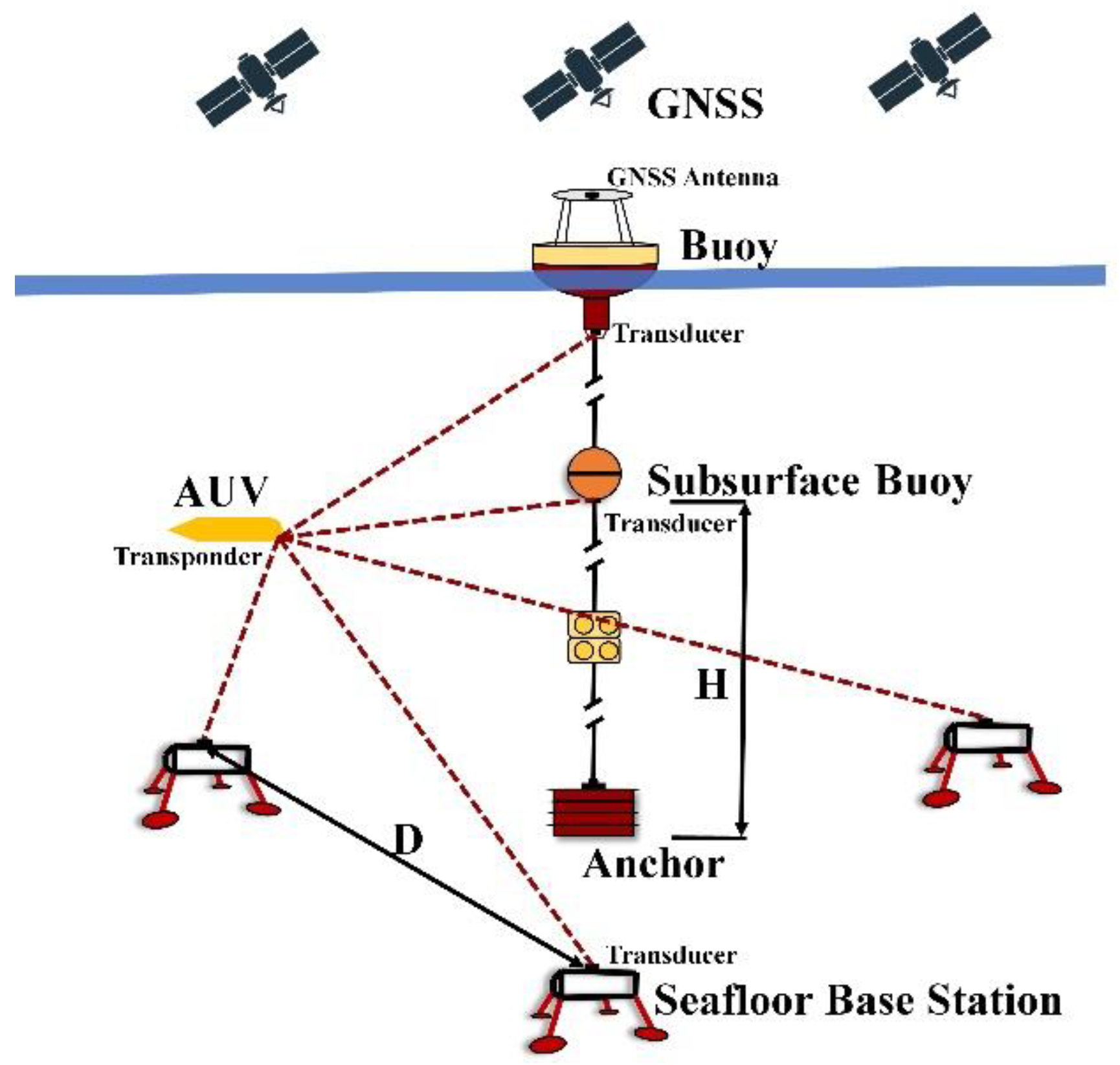
2.1. Underwater Geodetic Network Design

Figure 1 depicts the basic configuration of the underwater geodetic network (UGN). From bottom to top, we designed two acoustic systems: the seafloor system and the mooring system. The seafloor system comprises three base stations equipped with an omni-direction acoustic transducer. The mooring system consists of an anchor, rope, glass floats, and two buoys. The subsurface buoy is equipped with an omni-direction acoustic transducer, acoustic ranging controller, and battery. The moored sea surface buoy is equipped with an omni-direction acoustic transducer, acoustic ranging controller, battery, satellite communication module, and control display unit. In the mooring system, the buoys are moored on the same rope, and the height of the subsurface buoy can be adjusted for different environments.
To obtain the position of the geodetic stations, various positioning methods can be applied. Utilizing the moving survey onboard vessels, GNSS-A observations can be performed to determine the absolute coordinates of the seafloor base stations [1,27]. The subsurface buoy position can then be determined by ranging to the seafloor base stations [18]. Wave gliders or ASVs can also be auxiliary measurement platforms to provide GNSS-A observations and position the subsurface buoy [22,24,25]. The network configuration is also expandable. The subsurface buoy can be equipped with an inertial measurement unit (IMU) to account for its motion with the ocean currents or mooring rope. The sea surface buoy can be equipped with a GNSS receiver and antenna to determine its position [23]. Finally, the underwater submersible user, such as a near-bottom ROV or AUV, can obtain its location by receiving the acoustic signals from UGN [12,32].
In this study, the basic network configuration, which consists of three seafloor base stations, one subsurface buoy, and one surface buoy, is expressed as the “3 seafloor base stations + 1 subsurface buoy + 1 sea surface buoy” (“3+1+1”) configuration. The seafloor base stations are distributed evenly on a circle, and the distance between the seafloor base stations is set as D. The subsurface buoy is located above the horizontal center of the seafloor base station array with a vertical height of H (0 < H ≤ 3000 m), while the sea surface buoy is about 3000 m above the seafloor array center. Note that the basic configuration can be expanded or reduced to other configurations, such as the “4 seafloor base stations + 1 subsurface buoy + 1 sea surface buoy” configuration, “3 seafloor base stations + 0 subsurface buoy + 1 sea surface buoy” configuration, and so on. The network dimension, its positioning range, and kinematic positioning performance at different undersea points are closely related to the seafloor station separation and the subsurface buoy height. Therefore, the performance of the network configuration in the underwater space should be evaluated.

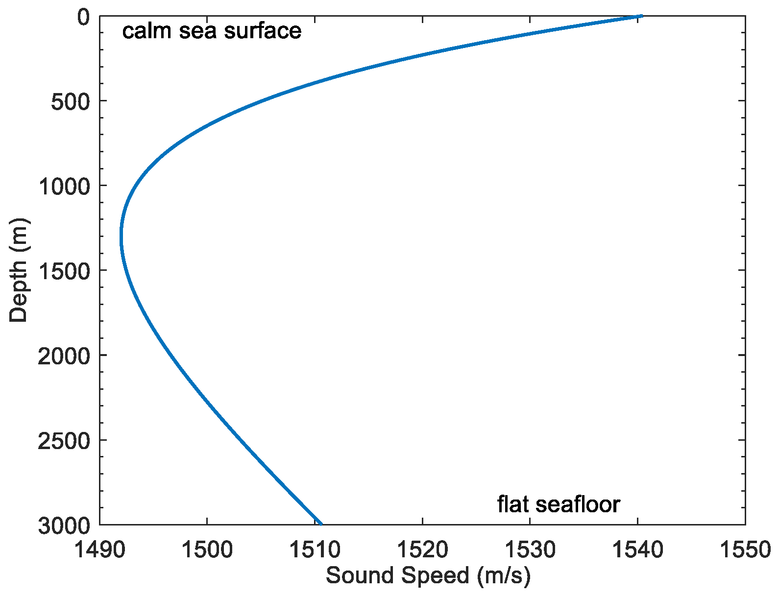
2.2. Underwater Environmental Factors

The network configuration is the primary focus of our study. Generally, the seafloor topography, ocean currents, tides, internal waves, sea surface wind, sound speed variation, and other environmental factors all have an impact on the network kinematic positioning performance. The acoustic signal propagation bending always causes sound rays to sweep the seafloor, affecting acoustic signal propagation [15,33]. In the construction of an UGN, its height should be designed considering the seafloor topography and seabed sediment. Ocean currents and internal waves can affect the stability of the subsurface buoy [29], and the height of the subsurface buoy must be optimized. Similarly, waves and tides affect the stability of the sea surface buoy, and its position error also needs to be considered [21,23]. In addition, the coordinate error and clock drift of network base stations also influence the kinematic positioning performance. Similar to GNSS, the impact of underwater environmental factors can be classified as User Equivalent Range Errors (UEREs), while the station coordinate and clock errors are considered as Signal-In-Underwater-Space Range Errors (SISREs) [34]. The impact of underwater environmental factors is evaluated in Section 3.4.

2.3. Kinematic Positioning Performance Assessment Methods

To evaluate the kinematic positioning performance of the UGN, an underwater space with a depth of 3000 m and a horizontal range of 25 km × 25 km was simulated in grids, and the grid spatial resolution was 500 m on the horizontal and 200 m on the vertical. For ocean near-bottom surveying and precision engineering applications, the user can distribute at any vertex of the grids 100 m above the seafloor, and the total number of grids was 39,015.
The underwater user’s single-epoch kinematic positioning can be realized by receiving acoustic signals from UGN. The acoustic sonar properties and the underwater environment influence the kinematic positioning performance. Considering the current acoustic ranging technology [13,32], the omni-direction acoustic sonar’s operating frequency is 8~16 kHz, and the maximum positioning range of one network station can reach 10 km with the same precision at a depth of 3000 m. Additionally, the time delay measurement error was set to 0.1 ms, which was equivalent to the ranging error of approximately 0.15 m. To simplify the impact of the underwater environment, only the constant sound speed error of 0.1 m/s was considered in the simulation [35].
In terms of the positioning range and precision, the Available Station Number (ASN), Effective Positioning Grid (EPG), and Position Dilution of Precision (PDOP) indicators are considered.
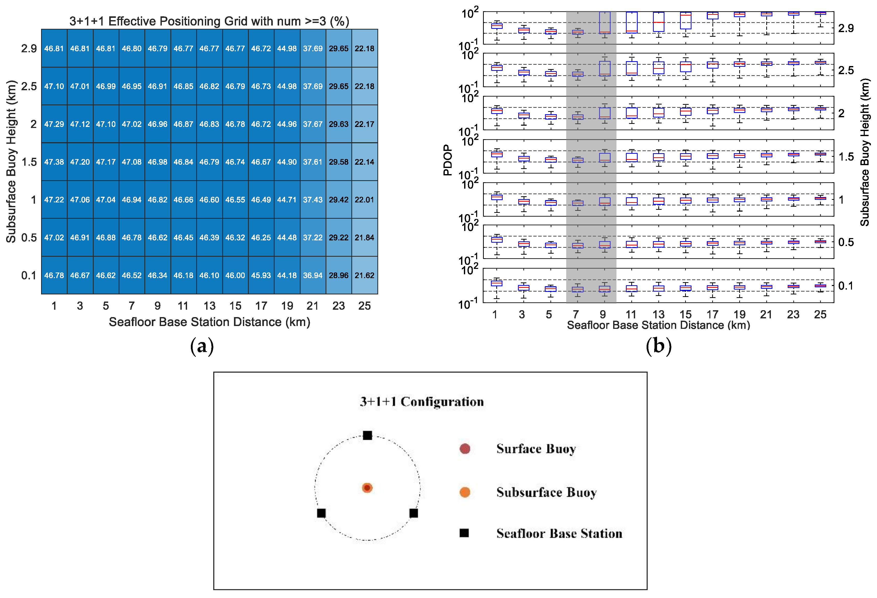
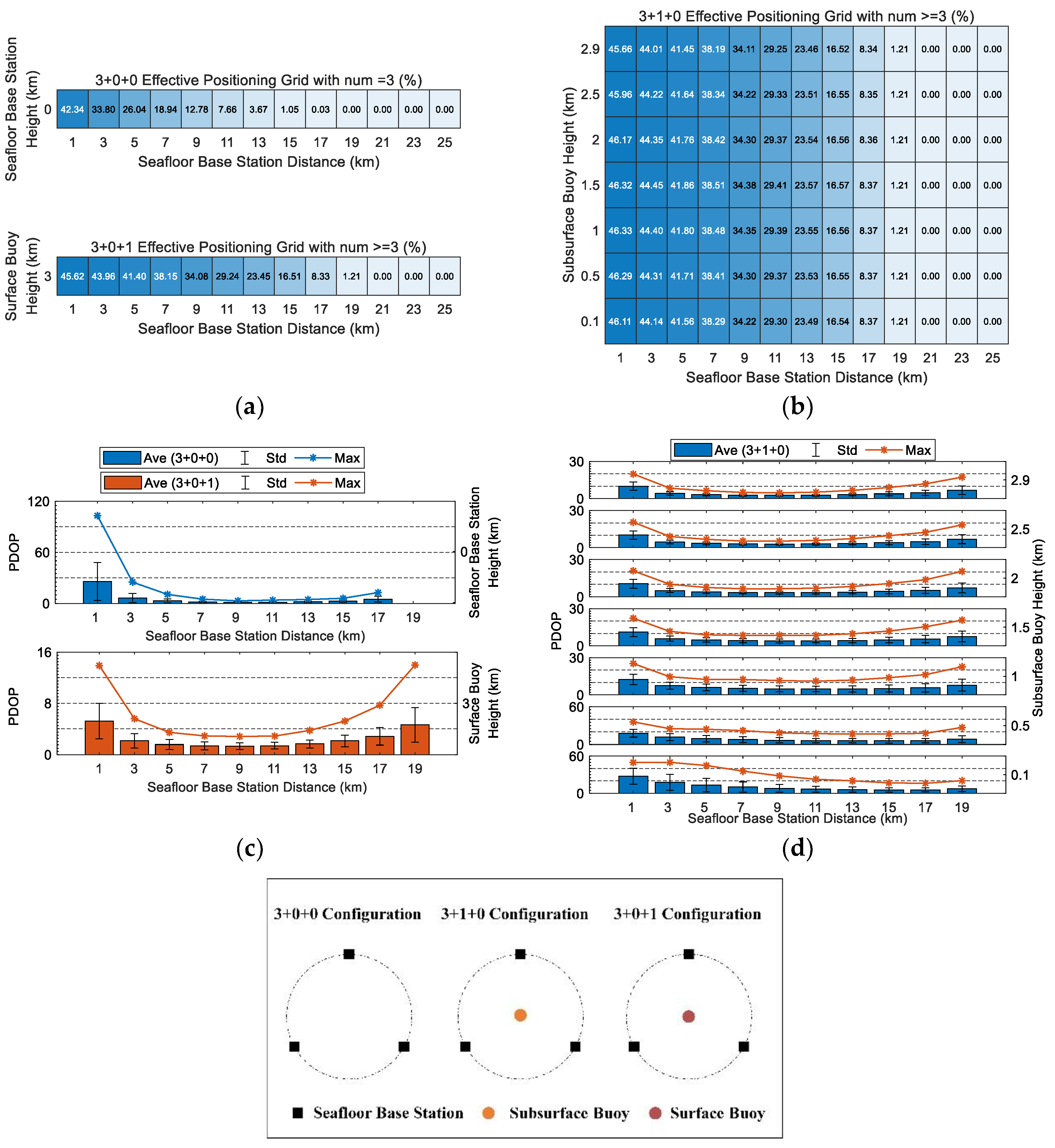
  • Available Station Number (ASN) and Effective Positioning Grid (EPG)
For the user’s random position, the Euclidean distance between the user and the station (seafloor base station, subsurface buoy, or sea surface buoy) is set to L . If 0 < L 10   k m , then the user is within the effective positioning range of a station, and we consider this station as an available station for this user grid point; otherwise, it is unavailable. For different user grid points, the available station number (ASN) is variable.
Similar to GNSS, if the sonar signal delay is ignored and the clock of the synchronization-type sonar is precisely synchronized, the user single-epoch kinematic positioning can be achieved by receiving acoustic signals from at least 3 stations (seafloor base stations and/or buoys). We defined the Effective Positioning Grid (EPG) as the user grid point with at least 3 available station numbers (ASNs). Therefore, the EPG index is intended to evaluate the effective positioning range of the network configuration in the underwater space.
  • Position Dilution of Precision (PDOP)
To realize user single-epoch kinematic positioning, the least-squares adjustment can be applied, and the basic positioning model is
l i j = L i j ( x i ) + v i j L i j ( x ) = c j x i 2 = k = 1 3 ( x i , k c j , k ) 2
where l i j is the acoustic measurement in distance between user i and station j , L i j ( x i ) is the Euclidean distance, v i j is the distance error, and x i and c j are the positions of user i and station j , respectively.
The linearization of the Equation (1) is
v i j = e i j δ x i ( l i j L i j ( x i 0 ) ) e i j = [ c j , 1 x i , 1 0 ,   c j , 2 x i , 2 0 ,   c j , 3 x i , 3 0 ] / c j x i 0 2
where δ x = x x 0 , and x 0 is the initial value of x .
Accumulating the acoustic measurements from all of the available stations, we obtain the error equations
V = B δ x L B = [ e i 1 T ,     e i 2 T ,     e i n   T ] T L = [ l i 1 L i 1 ( x 0 ) ,     l i 2 L i 2 ( x 0 ) ,         l i n L i n ( x 0 ) ] T
where δ x is the parameter to be estimated, B is the design matrix, and n is the available station number.
For user single-epoch kinematic positioning, we can evaluate the positioning accuracy σ X
σ X = tr [ ( B T P Β ) 1 ]     σ 0 = tr ( N 1 )     σ 0 P = σ 0 2 / ( σ r a n g i n g   e r r o r 2 + ( L ( x 0 ) / 1500 ) 2 σ s o u n d     s p e e d   e r r o r 2 )
where N is the normal matrix, P is the weight matrix, which considers the ranging error and the constant sound speed error, and σ 0 2 is the variance of unit weight [26,36]. The a posteriori variance of the unit weight is assumed to equal to the a priori variance of the unit weight in the adjustment model.
The positioning accuracy σ X is related to the network geometric structure formed by the user and network stations, which can be evaluated by the position dilution of precision PDOP [26]
PDOP = tr ( N 1 )
We analyzed the PDOP in the underwater space using Equations (6)–(8), where m is the number of all grid points. The maximum PDOP determines the lower bound of the positioning accuracy.
Average PDOP:
PDOP ave = 1 m i = 1 m PDOP i
Standard deviation of PDOP:
PDOP std = 1 m 1 i = 1 m ( PDOP i PDOP mean ) 2
Maximum PDOP:
PDOP max = Max ( PDOP 1 , PDOP 2 , PDOP m )

3. Results and Discussion

3.1. Evaluation of Network Kinematic Positioning Performance

To evaluate the kinematic positioning performance of the basic network configuration “3+1+1”, various distances between the seafloor base stations and heights of the subsurface buoy were simulated. As the user can obtain single-epoch kinematic positioning by receiving acoustic signals from at least three stations, we analyzed the number of effective positioning grids (EPGs) and the position dilution of precision (PDOP) with at least three available station numbers (ASN). Figure 2a shows the percentage of EPGs in the total grid number of 39,015. For the same subsurface buoy height, the EPG varied significantly with the seafloor base station distance. When the distance was less than 17 km, the EPG decreased slowly as the distance increased. However, when the distance was greater than 17 km, the circumscribed circle radius of the seafloor base stations array was greater than 10 km, and the EPG decreased rapidly. For the same seafloor station distance, the EPG changed gently with the subsurface buoy height. The EPG values were relatively larger when the subsurface buoy height was above 1.5 km. Overall, the EPG reached its maximal value of 18,486 when the seafloor base station distance was 1 km and the subsurface buoy height was 1.5 km.
Figure 2b shows the PDOP value variation with the seafloor base station distance and the subsurface buoy height. According to Equation (5), due to the inversion of N, outliers of PDOP value may occur. We detected and removed the PDOP outlier when its value exceeded ±1.5 × IQR (interquartile range), which amounted to approximately 7% of all of the PODPs [37]. Figure 2b indicates that, when the subsurface buoy height is lower than 1.5 km, the PDOP value changes slowly with the base station distance. However, when the height is higher than 1.5 km and the distance changes from 7 km to 9 km, the PDOP values change notably. Overall, the results show that, when the subsurface buoy height is less than 1.5 km, the PDOP mainly changes with the seafloor base station distance. Otherwise, the PDOP fluctuates with the subsurface buoy height and the station distance.

3.2. Impact of Network Dimension on Positioning Performance

For the “3+1+1” configuration, the dimensions relate to the distance between the seafloor base stations and the height of the subsurface buoy. The EPGs of different dimensions can be scattered or concentrated in the underwater space. We need to analyze the impact of the seafloor base station distance and subsurface buoy height on the user positioning range, available station number, and positioning accuracy.
Figure 3a shows the EPG values with various available stations in the “3+1+1” network configuration. We defined EPGs with 3, 4, and 5 available station numbers as EPG ASN = 3 , EPG ASN = 4 , and EPG ASN = 5 , respectively. For the convenience of comparison, we also expressed EPGs with 0, 1, and 2 available station numbers as EPG ASN = 0 , EPG ASN = 1 , and EPG ASN = 2 , respectively.
From Figure 3a, in general, the seafloor base station distance has a much greater impact on the EPG with different available station numbers than the subsurface buoy height. When the height was constant, EPG ASN = 0 decreased with the increase in distance; when the distance was 13~19 km, EPG ASN = 0 tended to be stable. However, EPG ASN = 0 gradually increased when the distance was greater than 19 km. Due to the limited acoustic positioning range (10 km), there were always grid points with unavailable base stations. EPG ASN = 1 increased with the distance at first; when the distance was close to 11 km, EPG ASN = 1 was stable; when the distance was greater than 19 km, EPG ASN = 1 showed a decreasing trend. EPG ASN = 2 was significantly lower than the others, and EPG ASN = 2 began to increase when the distance was greater than 19 km. EPG ASN = 3 increased with the distance at first; when the distance approached 19 km, EPG 3 reached the maximum value and then decreased. EPG ASN = 4 was similar to EPG ASN = 3 , while the maximum value of EPG ASN = 4 occurred when the distance was close to 11 km, and EPG ASN = 4 disappeared with distances greater than 19 km. EPG ASN = 5 showed a downward trend with the distance. When the distance was greater than 17 km, the distance between the seafloor base stations exceeded the maximum acoustic range (10 km), and user positioning with five stations was no longer possible.
Figure 3b shows the average, standard deviation, and maximum values of PDOP. PDOP was inversely proportional to the geometric structure formed by the user and stations, and the user positioning accuracy based on the network configuration was affected by the seafloor base station distance and the subsurface buoy height. After the removal of outliers with the IQR criterion, most PDOP values were less than 30, except for when the height was above 2.5 km. We found that PDOP outliers appeared when users were located near the seafloor base stations. Moreover, when the height was lower than 1.5 km, the PDOP value changed slowly with the seafloor base station distance. When the distance increased from 7 km to 9 km, the variation of PDOP was obvious.
Since the subsurface buoy height had little impact on EPG, we investigated the spatial distribution of the EPG with the fixed subsurface buoy height and various seafloor base station distances (Figure 3c,d). The height was fixed at 2.9 km, and the distances were 7 km and 9 km, respectively. In both scenarios, grids with five available stations covered the station array, and grids with three and four available stations were outside the station array. It is obvious that they were all within a circle in the plane, and the radius was approximately 10 km. Because the subsurface buoy and surface buoy were above the horizontal center of the seafloor base station array, grids with at least three available base stations were widely distributed. While grids with two available stations were only sporadically distributed, grids with one or unavailable base stations were distributed at the edge of the underwater space, where the acoustic ranging signal of the subsurface buoy and the surface buoy could not reach. When the station distance increased from 7 km to 9 km, EPG ASN = 0 and EPG ASN = 2 decreased by 27.63% and 3.82%; EPG ASN = 1 , EPG ASN = 3 , and EPG ASN = 4 increased by 19.40%, 45.83%, and 10.85%, respectively; while EPG ASN = 5 decreased by 86.63%, which was primarily linked to the obvious variation in the PDOP.
Based on the above analysis, for the “3+1+1” network configuration, the seafloor base station distance of 9~13 km and the subsurface buoy height of lower than 2.5 km were optimal in terms of positioning range and positioning accuracy. Considering Equation (4), the submersible positioning accuracy was less than 30 m within an underwater space of 25 km × 25 km × 3 km.

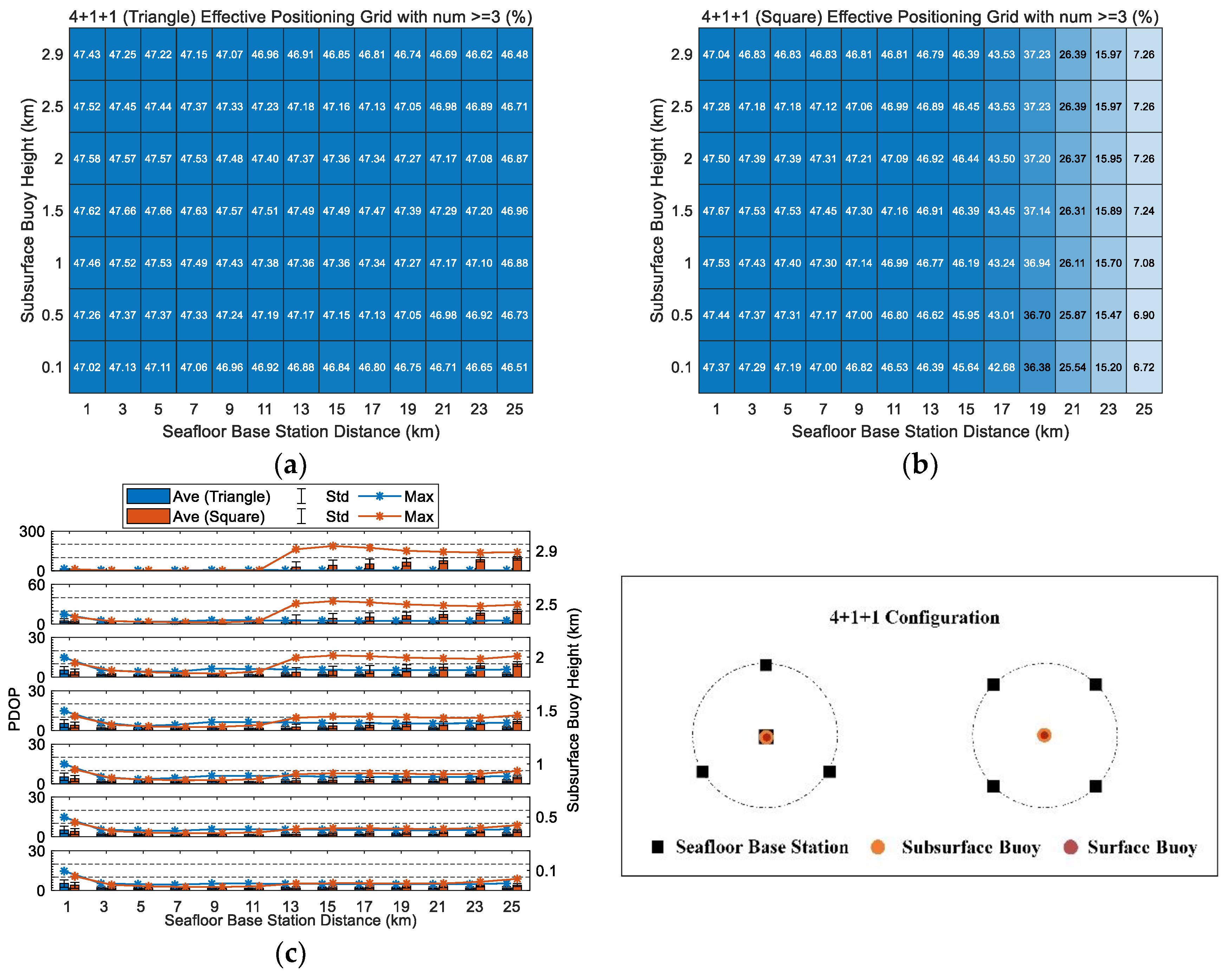
3.3. Impact of Network Configuration on Positioning Performance

3.3.1. Configuration without Buoys

To analyze the contribution of the underwater subsurface buoy and sea surface buoy to user positioning, we compared the network configurations “3 seafloor base stations + 0 subsurface buoy + 0 sea surface buoy” (“3+0+0”), “3 seafloor base stations + 0 subsurface buoy + 1 sea surface buoy” (“3+0+1”), and “3 seafloor base stations + 1 subsurface buoy + 0 sea surface buoy” (“3+1+0”).
We analyzed EPGs with at least three available stations ( EPG ASN 3 ). Figure 4a shows that the EPG ASN 3 of the “3+0+0” network configuration gradually decreased as the distance increased. When the distance was greater than 17 km, the available station number was not enough for positioning. For the “3+0+1” network configuration with the sea surface buoy, the EPG 3 values were much larger than those of the “3+0+0” network configuration. However, when the distance was greater than 19 km, the available station number was also not enough for positioning. Figure 4b shows that, for the “3+1+0” network configuration, by replacing the sea surface buoy with the subsurface buoy, the EPG 3 values had a similar situation. Compared with Figure 2a, for the “3+1+1” network configuration, it can be found that the EPG ASN 3 values increased significantly when the sea surface buoy and subsurface buoy were configured simultaneously. Moreover, when the distance was greater than 19 km, the proportion of EPG ASN 3 was still greater than >21%.
Figure 4c,d show the average, standard deviation, and maximum values of PDOP. PDOP outliers were removed if the PDOP value exceeded ±1.5 × IQR. For the “3+0+0” network configuration, the PDOP statistics first decreased and then increased as the distance increased. For the “3+0+1” network configuration, the PDOP values also had similar trends, but decreased significantly with the surface buoy. When we replaced the surface buoy with the subsurface buoy, and when the height of the buoy was greater than 1 km, the PDOP values decreased first and then increased as the distance increased; when the height was less than 1 km, the PDOP values also decreased with increasing distance. When the buoy height was less than 2.5 km, the PDOP average and standard deviation of the “3+1+0” network configuration were greater than those of the “3+1+1” network configuration. Moreover, when the subsurface buoy of the “3+1+0” network configuration was close to the sea surface, the positioning indicators were close to the “3+0+1” network configuration, and there was no significant difference between the functions of the subsurface buoy and the sea surface buoy.
In general, configurations without subsurface or surface buoys were unable to achieve positioning when the seafloor station distance exceeded 19 km, which can be avoided in the “3+1+1” network configuration with a subsurface buoy and sea surface buoy. In addition, the height of the subsurface buoy can be adjusted to improve the performance of the geodetic network. Therefore, the subsurface buoy is a necessary and important component to make UGNs more resilient and precise.
Although the sea surface buoy and the subsurface buoy had similar performances in kinematic positioning, the surface buoy could be equipped with a satellite communication module for transmitting the UGN data, receiving remote-control commands, etc. Moreover, the GNSS equipment on the surface buoy can be used for the clock synchronization of acoustic equipment, and the acoustic signal from the buoy can send time synchronization information to other stations in the UGN, which is crucial to maintaining accurate system time synchronization.

3.3.2. Configuration with More Seafloor Base Stations

Generally, four seafloor base stations are used in traditional networks [3,28], and the basic “3+1+1” network configuration can be expanded to the “4 seafloor base stations + 1 subsurface buoy + 1 sea surface buoy” (“4+1+1”) network configuration. Figure 5 illustrates this expanded configuration. We analyzed two kinds of seafloor base station array geometries, the triangular-center-form array geometry and the square-form array geometry.
Figure 5a,b show that, for the “4+1+1” network configurations, the EPG ASN 3 values fluctuated slightly when the base station distance was less than 19 km. Compared with the “3+1+1” network configuration (Figure 2a), when the distance was greater than 19 km, the EPG ASN 3 of the “4+1+1” network configuration (triangular-center-form array geometry) showed an obvious increase, and the percentage of EPG ASN 3 changed from 21.62% to 46.51%. In contrast, the EPG ASN 3 values of the “4+1+1” network configuration (square-form array geometry) decreased significantly, and the minimum percentage of EPG ASN 3 was 6.72%.
Figure 5c,d show that, when the distance was less than 13 km, the PDOP values of the triangular-center-form array geometry were slightly greater than those of the square-form array geometry. When the distance was greater than 13 km, the PDOP values of the square-form array geometry increased significantly and were greater than those of the triangular-center-form array. Moreover, compared with the “3+1+1” network configuration (Figure 3b), the PDOP values of the expanded network configuration (square-form array geometry) showed similar trends, but decreased slightly.
In general, the performance of positioning range and positioning accuracy can be improved by increasing the number of seafloor base stations. The improvement of kinematic positioning performance is also closely related to the array geometry. However, more seafloor base stations always mean more costs in equipment, construction, and maintenance. To optimize the cost and efficiency of the UGN, the basic “3+1+1” network configuration is more appropriate.

3.4. Impact of Acoustic Transmission Characteristics on Acoustic Signal Propagation

In the simulation section, the Euclidean distance between the base station and the user is adopted. However, the acoustic ray bending in the acoustic signal propagation path should be considered. Additionally, the acoustic transmission characteristics, such as the multipath effect caused by the acoustic signal reflected from the seabed or the sea surface, the Doppler effect caused by the motion of the acoustic source, and the transmission loss of acoustic energy, also affect acoustic signal propagation in the underwater environment. Herein, we simulated the acoustic transmission characteristics by BELLHOP [38] and studied the impact on acoustic signal propagation. The frequency of the omni-direction acoustic sonar was set to 8 kHz, and the users were randomly distributed in an underwater space of 3000 m in depth. To illustrate the impact on acoustic signal propagation, the signal service range was limited to 30 km in the horizontal, which was different from the signal positioning range in Section 2.3. Note that it is complex to simulate the real underwater environment, such as the temporal–spatial-varying ocean sound speed, sea surface wind and waves, and the seafloor topography. In the simulation, the typical deep-sea Munk model was used as the reference sound velocity profile [39], and a calm sea surface and flat seafloor were considered, as shown in Figure 6.

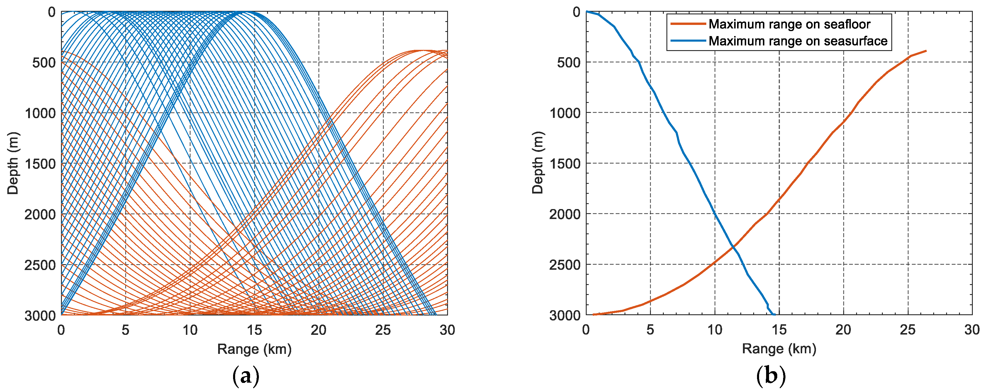
3.4.1. Acoustic Ray Bending

We first studied the direct acoustic signal from the base station to the user, excluding the reflected signal from the seafloor or the sea surface. Due to acoustic ray bending, there was an acoustic shadow where the sound signal could not reach. By finding the critical reversal point of the bending ray, where the ray grazed the horizontal, we referred to the horizontal distance between the reversal point and the base station as the maximum service range. For the fixed base station, when the user was within the maximum range, the acoustic signal could reach the user directly by adjusting the initial grazing angle; when the user was outside the maximum range, there existed the acoustic shadow. Therefore, we could investigate the impact of acoustic ray bending on the maximum service range.
The relationship between the initial grazing angle α s o u r c e of the acoustic signal at the base station and the grazing angle α r e v e r s a l at the reversal point is as follows [40]:
p = cos α s o u r c e c s o u r c e = cos α r e v e r s a l c r e v e r s a l α s o u r c e = arccos c s o u r c e c r e v e r s a l               ( α r e v e r s a l = 0 )  
where p is the ray constant, c is the sound speed, and α is the angle of the ray with respect to the horizontal, for which the upward angle is negative and the downward angle is positive.
Using the initial grazing angle α s o u r c e , the horizontal distance x between the reversal point and the base station is calculated by the 2-D planar ray-trace method, as follows [40]:
x = i = 1 n x i = i = 1 n [ 1 ( p c i ) 2 ] 1 / 2 [ 1 ( p c i + 1 ) 2 ] 1 / 2 p g i
where g is the gradient of the sound speed, n is the number of layers from the source to the reversal point.
Figure 7a shows the acoustic propagation path of the base station at different depths, and acoustic rays graze the sea surface and the seafloor, respectively. For the rays that grazed the sea surface, fixing the base station and decreasing the initial grazing angle of the upward acoustic signal, the ray could reach the area within the maximum service range on the sea surface. In contrast, when the initial grazing angle of the upward acoustic signal increased, the reversal point was away from the sea surface, and the ray could not reach the area between the reversal point and the sea surface. For the ray that grazed the seafloor, the situation was similar to that of the ray that grazed the sea surface. When the base station was fixed, the ray could reach the area within the maximum service range on the seafloor by increasing the initial grazing angle of the downward acoustic signal. In contrast, when the initial grazing angle of the upward acoustic signal decreased, the reversal point was away from the seafloor, and the ray could not reach the area between the reversal point and the seafloor.
Figure 7b shows the maximum service range on the sea surface and the seafloor, and the maximum range varied with the depth of the base station. For the maximum service range on the sea surface, it gradually increased with increasing depth. Decreasing the height of the subsurface buoy could increase the maximum service range on the sea surface, and the maximum service range of the seafloor base station was close to 15 km. For the maximum service range on the seafloor, the ray grazed on the seafloor when the sound speed satisfied c s o u r c e c r e v e r s a l according to Equation (9). For the Munk sound velocity profile, the sound speed in the water shallower than 400 m could not satisfy the condition, and the rays from the depth of 0~400 m were reflected or absorbed at the seafloor. When the depth was greater than 400 m, the sound speed satisfied the condition, and the ray could graze on the seafloor. The maximum service range on the seafloor gradually decreased as the depth increased, and the ray was refracted upward when the base station was on the seafloor, for which the maximum service range on the seafloor was 0 m and not plotted.
In general, the effect of ray bending on the service range can be reduced by lifting the station height. For the seafloor base station, increasing the erection height is costly and laborious, and weakens the stability of the station. Therefore, subsurface buoys can be an alternative station to the seafloor base station to increase the service range. In addition, this study only considered the case of flat seafloor, and the effects of seafloor topographic features, such as steep slopes and sea hills, will be considered in future studies.

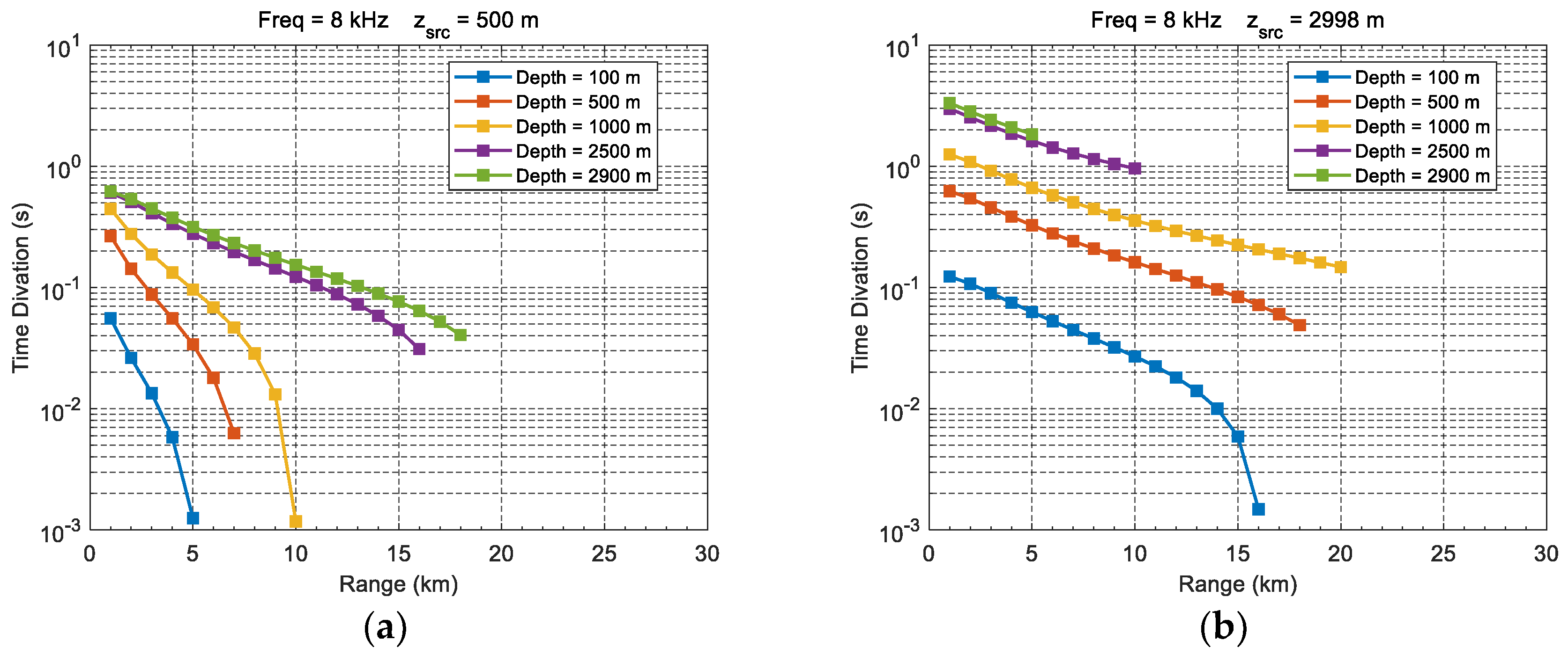
3.4.2. Multipath and Doppler Effects

Multipath signals, such as reflected signals from the seabed, the sea surface, the equipment, etc., affect acoustic signal propagation [19], and misrecognizing reflected signals as direct signals also leads to acoustic time delay errors [41]. The time deviation of the reflected signal from the direct signal was simulated by BELLHOP for base station depths of 500 m and 2998 m, as shown in Figure 8a,b. The results show that the multipath signals caused time deviations of milliseconds to seconds. In general, methods such as the signal cross-correlation function (CCF) accompanied by the Energy Ratio (ER) algorithm and Phase-Correlation-Only (PCO) method can be utilized to identify the direct acoustic signal from the multipath signal [19,20,21,41,42].
Figure 8a,b also show that the propagation time deviation decreased with increasing distance between the base station and the user. For a fixed user, the propagation time deviations of the shallow base station are significantly less than those of the deep base station. Therefore, the subsurface buoy helps to reduce the propagation time deviation. However, for the impact of decreasing the time deviation, on the one hand, the time deviation can be neglected when its value is close to a microsecond; on the other hand, it’s hard to distinguish the multipath signal when a sub-millisecond time deviation exists [19,21,43]. Nevertheless, these cases were not present in the simulation.
In addition, the acoustic signal cannot reach the user directly due to ray bending; e.g., with the seafloor base station at 2998 m depth and the user at 2900 m depth, there was no direct acoustic signal when the horizontal distance was more than 5 km. In contrast, the acoustic signal from the subsurface buoy of 500 m depth could reach the user directly under the same conditions, which also shows that the deployment of a subsurface buoy could increase the service range.
Due to the relative motion between the target and the base station, the acoustic signal generated a Doppler shift. During acoustic signal detection, the optimal frequency shift rate of the signal was generally estimated by searching the maximum cross-correlation coefficient to correct for the effect of the Doppler shift [20].
In general, both multipath and Doppler effects can be weakened or corrected during acoustic signal detection, which is beyond the scope of this paper and will be considered in further studies.

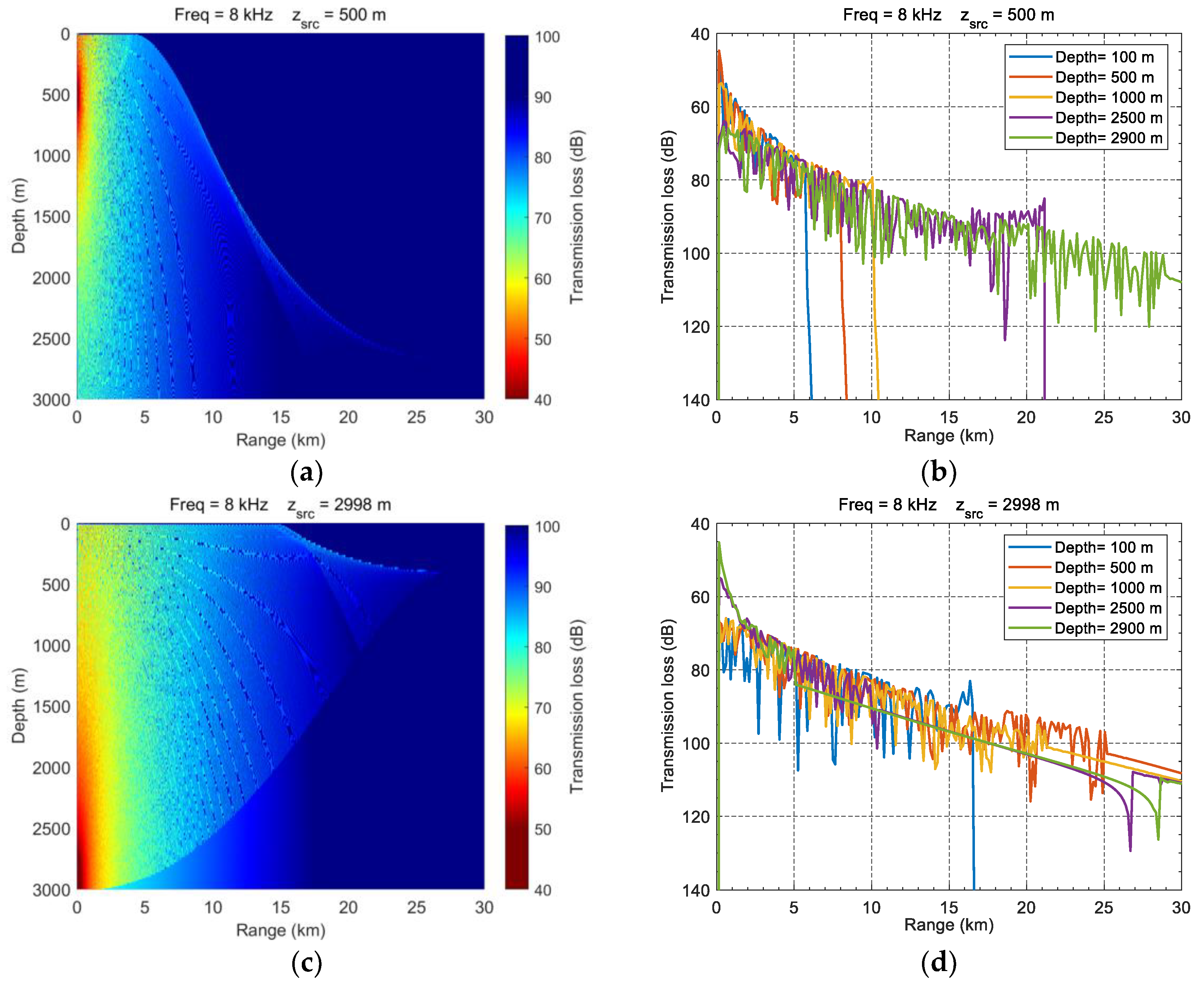
3.4.3. Acoustic Transmission Loss

Multipath signals also result in acoustic energy transmission loss ( T L ), and the transmission loss of the acoustic signal can be assessed as follows [38]:
T L ( d , f ) = k × 10 log ( d ) + 0.11 f 2 1 + f 2 + 44 f 2 4100 + f 2 + 3 × 10 4 f 2 + 3.3 × 10 3
where d is the distance between the station and the user, f is the signal frequency, and coefficient k represents the propagation geometry space.
Figure 9a,b show the transmission loss when the base station was at a depth of 500 m. Figure 9a shows that the transmission loss increased from 40 dB to 80 dB within the horizontal distance of 5 km. The transmission loss then increased slowly and approached 100 dB when the horizontal distance was 10 km. However, there was an obvious caustic curve above the depth of 2500 m—the transmission loss changed significantly from the left side of the curve to the right side. On the right side of the caustic curve, the rays reflected by the seafloor or the sea surface with large reflection loss, and the zone of large transmission loss decreased with increasing station depth. Therefore, for the station in shallow water, such as a subsurface buoy, the acoustic signals had a large transmission loss in the shallow water. Figure 9b shows the rapid increase in the transmission loss. When the user was at the depth of 100 m, there was a drastic change in the transmission loss at a horizontal distance of 6 km, while the drastic change occurred at a horizontal distance of 10.5 km when the user was at the depth of 1000 m.
Figure 9c,d show the transmission loss when the base station was at a depth of 2998 m. Figure 9c shows that, when the horizontal distance was within 2.5 km, the transmission loss gradually increased from 40 dB to 70 dB, and then the increase in the transmission loss slowed down. When the horizontal distance was 15 km, the transmission loss was close to 100 dB. Two obvious caustic curves could be found, and the depth of the turning point was about 500 m. For the caustic curve above 500 m, the zone of large transmission loss decreased with increasing station depth. In contrast, the zone of large transmission loss increased with increasing station depth for the other caustic curve. Figure 9d shows the rapid increase in the transmission loss when the base station was at a depth of 2998 m. When the user was at a depth of 100 m, the horizontal distance of drastic change increased to 16.5 km, and when the user was at a depth of 1000 m, the horizontal distance increased to 21.5 km. Therefore, for the base station in deep water, the acoustic signals had a large transmission loss in both shallow and deep water.
From the above analysis, when the base stations were located at 500 m and 2998 m depths simultaneously, they could compensate for the signal transmission loss in shallow and deep water, which further indicates the necessity of deploying the subsurface buoy and seafloor base stations.

4. Conclusions

Our study proposes an underwater geodetic network configuration consisting of three seafloor base stations, one underwater subsurface buoy, and one sea surface buoy. The main purpose of the UGN is to provide kinematic positioning for regional underwater submersibles for ocean near-bottom surveying and precision engineering. To evaluate the performance of the network configuration, the positioning range and accuracy were analyzed by changing the seafloor base station separation and subsurface buoy height. The simulation results indicated that, in a deep-sea environment with a water depth of 3000 m, the positioning accuracy and range were mainly affected by the distance between the seafloor base stations, and the height of the subsurface buoy had a greater impact on the positioning accuracy than on the positioning range. In general, when the distance between seafloor base stations was 9~13 km and the height of the subsurface buoy above the seafloor was lower than 2.5 km, the configuration had the optimal kinematic positioning performance, which could achieve a submersible positioning accuracy of less than 30 m within an underwater space of 25 km × 25 km × 3 km. Compared with the network configurations with fewer or more stations, the proposed configuration with the underwater subsurface buoy and the sea surface buoy made the kinematic positioning performance of the UGN more precise and cost-effective.
The purpose of our study was to evaluate the configuration of UGNs on kinematic positioning performance. Based on the proposed evaluation method in this study, an optimal network configuration with the best positioning performance can be obtained under various conditions, such as the effective sonar ranging distance and accuracy, the water depth, and the underwater base station configuration. However, a variety of other factors, including the underwater acoustic environment, the base station coordinate accuracy, and stability, affect the user kinematic positioning performance, which should be thoroughly investigated in future studies.

Author Contributions

Conceptualization, M.L., Y.L. (Yang Liu), Y.L. (Yanxiong Liu) and Y.H.; methodology, M.L. and Y.L. (Yang Liu); coding, M.L.; validation, M.L., Y.L. (Yang Liu), Y.L. (Yanxiong Liu) and G.C.; formal analysis, M.L., Y.L. (Yang Liu), Y.L. (Yanxiong Liu) and G.C.; writing—original draft preparation, M.L.; writing—review and editing, Y.L. (Yang Liu), Y.L. (Yanxiong Liu), G.C. and Q.T.; visualization, M.L.; supervision, Y.L. (Yang Liu) and Y.L. (Yanxiong Liu); funding acquisition, Y.L. (Yang Liu), Y.L. (Yanxiong Liu) and Y.W. All authors have read and agreed to the published version of the manuscript.

Funding

This research was funded by the National Key Research and Development Program of China, grant number 2020YFB0505805, the National Natural Science Foundation of China, grant numbers 42004030 and 41974001, Wenhai Program of the S&T Fund of Shandong Province for Pilot National Laboratory for Marine Science and Technology (Qingdao), grant number 2021WHZZB1002 and Technology Innovation Pilot Program of Shandong Province, grant number 2020YFB0505800.

Data Availability Statement

The data presented in this study are available on request from the corresponding author.

Acknowledgments

We thank Xiaoru Xie at Ocean University of China for her help in figure generation and analysis. We greatly appreciate the anonymous reviewers for the insightful comments that improved this manuscript greatly.

Conflicts of Interest

The authors declare no conflict of interest.

References

  1. Yang, Y.; Liu, Y.; Sun, D.; Xu, T.; Xue, S.; Han, Y.; Zeng, A. Seafloor geodetic network establishment and key technologies. Sci. China Earth Sci. 2020, 50, 936–945. [Google Scholar] [CrossRef]
  2. Batista, P.; Silvestre, C.; Oliveira, P. A Sensor-based Long Baseline Position and Velocity Navigation Filter for Underwater Vehicles. IFAC Proc. Vol. 2010, 43, 302–307. [Google Scholar] [CrossRef] [Green Version]
  3. Zhang, J.; Han, Y.; Zheng, C.; Sun, D. Underwater target localization using long baseline positioning system. Appl. Acoust. 2016, 111, 129–134. [Google Scholar] [CrossRef]
  4. Spiess, F.N. Analysis of a possible sea floor strain measurement system. Mar. Geod. 1985, 9, 385–398. [Google Scholar] [CrossRef]
  5. Spiess, F.N.; Chadwell, C.D.; Hildebrand, J.A.; Young, L.E.; Purcell, G.H., Jr.; Dragert, H. Precise GPS/Acoustic positioning of seafloor reference points for tectonic studies. Phys. Earth Planet. Inter. 1998, 108, 101–112. [Google Scholar] [CrossRef]
  6. Chadwell, C.D. Shipboard towers for Global Positioning System antennas. Ocean Eng. 2003, 30, 1467–1487. [Google Scholar] [CrossRef]
  7. Gagnon, K.; Chadwell, C.D.; Norabuena, E. Measuring the onset of locking in the Peru-Chile trench with GPS and acoustic measurements. Nature 2005, 434, 205. [Google Scholar] [CrossRef] [PubMed]
  8. Chadwell, C.D.; Spiess, F.N. Plate motion at the ridge-transform boundary of the south Cleft segment of the Juan de Fuca Ridge from GPS-Acoustic data. J. Geophys. Res. Solid Earth 2008, 113, B04415. [Google Scholar] [CrossRef] [Green Version]
  9. Yang, Y.; Qin, X. Resilient observation models for seafloor geodetic positioning. J. Geod. 2021, 95, 79. [Google Scholar] [CrossRef]
  10. Techy, L.; Morganseny, K.A.; Woolseyz, C.A. Long-baseline acoustic localization of the Seaglider underwater glider. In Proceedings of the 2011 American Control Conference, San Francisco, CA, USA, 29 June–1 July 2011; pp. 3990–3995. [Google Scholar]
  11. Iinuma, T.; Kido, M.; Ohta, Y.; Fukuda, T.; Tomita, F.; Ueki, I. GNSS-Acoustic Observations of Seafloor Crustal Deformation Using a Wave Glider. Front. Earth Sci. 2021, 9, 600946. [Google Scholar] [CrossRef]
  12. Kinsey, J.; Eustice, R.; Whitcomb, L. A Survey of Underwater Vehicle Navigation: Recent Advances and New Challenges. In Proceedings of the Conference of Manoeuvering and Control of Marine Craft, Lisbon, Portugal, 20–22 September 2006; pp. 1–12. [Google Scholar]
  13. Sun, D.; Zheng, C.; Zhang, J.; Han, Y.; Cui, H. Development and Prospect for Underwater Acoustic Positioning and Navigation Technology. Bull. Chin. Acad. Sci. 2019, 34, 331–338. [Google Scholar] [CrossRef]
  14. High-Depths USBL Positioning System. Available online: https://www.ixblue.com/products/posidonia (accessed on 10 April 2022).
  15. Sun, W.; Liu, Q.; Yin, X.; Liu, J. A method of calculating the maximum mutually measuring distances between the transponders. Hydrogr. Surv. Chart. 2019, 39, 10–13. [Google Scholar] [CrossRef]
  16. Alcocer, A.; Oliveira, P.; Pascoal, A. Underwater acoustic positioning systems based on buoys with GPS. In Proceedings of the Eighth European Conference on Underwater Acoustics, Carvoeiro, Portugal, 12–15 June 2006; Volume 8, pp. 1–8. [Google Scholar]
  17. Burgmann, R.; Chadwell, D. Seafloor Geodesy. Annu. Rev. Earth Planet. Sci. 2014, 42, 509–534. [Google Scholar] [CrossRef]
  18. Blum, J.A.; Chadwell, C.D.; Driscoll, N.; Zumberge, M.A. Assessing slope stability in the Santa Barbara Basin, California, using seafloor geodesy and CHIRP seismic data. Geophys. Res. Lett. 2010, 37, 438–454. [Google Scholar] [CrossRef]
  19. Imano, M.; Kido, M.; Ohta, Y.; Fukuda, T.; Ochi, H.; Takahashi, N.; Hino, R. Improvement in the Accuracy of Real-Time GPS/Acoustic Measurements Using a Multi-Purpose Moored Buoy System by Removal of Acoustic Multipath. In Proceedings of the International Symposium on Geodesy for Earthquake and Natural Hazards, Matsushima, Japan, 22–26 July 2014; pp. 105–114. [Google Scholar]
  20. Ikuta, R.; Tadokoro, K.; Ando, M.; Okuda, T.; Sugimoto, S.; Takatani, K.; Yada, K.; Besana, G.M. A new GPS-acoustic method for measuring ocean floor crustal deformation: Application to the Nankai Trough. J. Geophys. Res. Solid Earth 2008, 113, B02041. [Google Scholar] [CrossRef] [Green Version]
  21. Tadokoro, K.; Kinugasa, N.; Kato, T.; Terada, Y.; Matsuhiro, K. A Marine-Buoy-Mounted System for Continuous and Real-Time Measurment of Seafloor Crustal Deformation. Front. Earth Sci. 2020, 8, 123. [Google Scholar] [CrossRef]
  22. Kido, M.; Fujimoto, H.; Hino, R.; Ohta, Y.; Osada, Y.; Iinuma, T.; Azuma, R.; Wada, I.; Miura, S.; Suzuki, S. Progress in the Project for Development of GPS/Acoustic Technique Over the Last 4 Years. In Proceedings of the International Symposium on Geodesy for Earthquake and Natural Hazards (GENAH), Matsushima, Japan, 22–26 July 2014; Springer: Cham, Switzerland, 2015; pp. 3–10. [Google Scholar] [CrossRef]
  23. Imano, M.; Kido, M.; Honsho, C.; Ohta, Y.; Takahashi, N.; Fukuda, T.; Ochi, H.; Hino, R. Assessment of directional accuracy of GNSS-Acoustic measurement using a slackly moored buoy. Prog. Earth Planet. Sci. 2019, 6, 56. [Google Scholar] [CrossRef] [Green Version]
  24. Chadwell, C.D. GPS-Acoustic Seafloor Geodesy using a Wave Glider. In Proceedings of the AGU Fall Meeting, San Francisco, CA, USA, 9–13 December 2013; Volume 2013, p. G14A-01. [Google Scholar]
  25. Yokota, Y.; Matsuda, T. Underwater Communication Using UAVs to Realize High-Speed AUV Deployment. Remote Sens. 2021, 13, 4173. [Google Scholar] [CrossRef]
  26. Zhao, J.; Zou, Y.; Zhang, H.; Wu, Y.; Fang, S. A new method for absolute datum transfer in seafloor control network measurement. J. Mar. Sci. Technol. 2016, 21, 216–226. [Google Scholar] [CrossRef]
  27. Chen, G.; Liu, Y.; Liu, Y.; Liu, J. Improving GNSS-acoustic positioning by optimizing the ship’s track lines and observation combinations. J. Geod. 2020, 94, 61. [Google Scholar] [CrossRef]
  28. Nakamura, Y.; Yokota, Y.; Ishikawa, T.; Watanabe, S. Optimal Transponder Array and Survey Line Configurations for GNSS-A Observation Evaluated by Numerical Simulation. Front. Earth Sci. 2021, 9, 33. [Google Scholar] [CrossRef]
  29. Matsui, R.; Kido, M.; Niwa, Y.; Honsho, C. Effects of disturbance of seawater excited by internal wave on GNSS-acoustic positioning. Mar. Geophys. Res. 2019, 40, 541–555. [Google Scholar] [CrossRef]
  30. Watanabe, S.; Ishikawa, T.; Yokota, Y.; Nakamura, Y. GARPOS: Analysis Software for the GNSS-A Seafloor Positioning with Simultaneous Estimation of Sound Speed Structure. Front. Earth Sci. 2020, 8, 508. [Google Scholar] [CrossRef]
  31. Diamant, R.; Lampe, L. Underwater Localization with Time-Synchronization and Propagation Speed Uncertainties. IEEE Trans. Mob. Comput. 2013, 12, 1257–1269. [Google Scholar] [CrossRef]
  32. Norgren, P.; Skjetne, R. Using Autonomous Underwater Vehicles as Sensor Platforms for Ice-Monitoring. Model. Identif. Control 2014, 35, 263–277. [Google Scholar] [CrossRef] [Green Version]
  33. Liu, J.; Chen, G.; Zhao, J.; Gao, K.; Liu, Y. Development and Trends of Marine Space-Time Frame Network. Geomat. Inf. Sci. Wuhan Univ. 2019, 44, 17–37. [Google Scholar] [CrossRef]
  34. Warren, D.M.; Raquet, J. Broadcast vs. precise GPS ephemerides: A historical perspective. GPS Solut. 2003, 7, 151–156. [Google Scholar] [CrossRef]
  35. Kido, M.; Osada, Y.; Fujimoto, H. Temporal variation of sound speed in ocean: A comparison between GPS/acoustic and in situ measurements. Earth Planets Space 2008, 60, 229–234. [Google Scholar] [CrossRef] [Green Version]
  36. Xue, S.; Yang, Y. Positioning configurations with the lowest GDOP and their classification. J. Geod. 2015, 89, 49–71. [Google Scholar] [CrossRef]
  37. Beavan, J. Noise properties of continuous GPS data from concrete pillar geodetic monuments in New Zealand and comparison with data from U.S. deep drilled braced monuments. J. Geophys. Res. Solid Earth 2005, 110, B08410. [Google Scholar] [CrossRef]
  38. Morozs, N.; Gorma, W.; Henson, B.; Shen, L.; Mitchell, P.; Zakharov, Y. Channel Modeling for Underwater Acoustic Network Simulation. IEEE Access 2020, 8, 136151–136175. [Google Scholar] [CrossRef]
  39. Munk, W.H. Sound channel in an exponentially stratified ocean, with application to SOFAR. J. Acoust. Soc. Am. 1974, 55, 220–226. [Google Scholar] [CrossRef]
  40. Chadwell, C.D.; Sweeney, A.D. Acoustic Ray-Trace Equations for Seafloor Geodesy. Mar. Geod. 2010, 33, 164–186. [Google Scholar] [CrossRef]
  41. Sweeney, A.D.; Chadwell, C.D.; Hildebrand, J.A.; Spiess, F.N. Centimeter-Level Positioning of Seafloor Acoustic Transponders from a Deeply-Towed Interrogator. Mar. Geod. 2005, 28, 39–70. [Google Scholar] [CrossRef]
  42. Honsho, C.; Kido, M.; Ichikawa, T.; Ohashi, T.; Kawakami, T.; Fujimoto, H. Application of Phase-Only Correlation to Travel-Time Determination in GNSS-Acoustic Positioning. Front. Earth Sci. 2021, 9, 7. [Google Scholar] [CrossRef]
  43. Tadokoro, K.; Ikuta, R.; Watanabe, T.; Ando, M.; Okuda, T.; Nagai, S.; Yasuda, K.; Sakata, T. Interseismic seafloor crustal deformation immediately above the source region of anticipated megathrust earthquake along the Nankai Trough, Japan. Geophys. Res. Lett. 2012, 39, L10306. [Google Scholar] [CrossRef]
Figure 1. Schematic diagram of the underwater geodetic network configuration and user navigation application. The network consists of a seafloor component and a mooring component.
Remotesensing 14 01939 g001
Figure 2. User positioning indicators of the “3+1+1” network configuration. (a) Heat map of the percentage of EPGs with the number of available stations ≥3. (b) Box chart of the PDOP variation with the seafloor base station distance and the subsurface buoy height. The red line denotes the median, the blue box denotes IQR (interquartile range), the solid black lines denote the maximum value and minimum value, respectively, and the ±1.5 × IQR criterion is used for outlier detection and removal. The shaded area denotes the steep variation of the PODP.
Remotesensing 14 01939 g002
Figure 3. User positioning indicators under various distance and height conditions. (a) EPG with various available stations—the colors blue, orange, yellow, purple, green, and red indicate the available station numbers of 0~5, respectively; (b) changes in the average, standard deviation, and maximum of PDOP—the blue box denotes the average, the black vertical line denotes the standard deviation, and the orange asterisk line denotes the maximum value; (c,d) spatial distribution of the ASN when the subsurface buoy height is 2.5 km, and the seafloor base station distances are 7 km and 9 km, respectively.
Remotesensing 14 01939 g003
Figure 4. User positioning indicators of the “3+0+0”, “3+0+1”, and “3+1+0” network configurations. (a,b) Heat maps of the percentage of EPGs with the number of available base stations ≥3; (c,d) average, standard deviation, and maximum PDOP—the box denotes the average, the black vertical line denotes the standard deviation, and the asterisk line denotes the maximum value. The results for the “3+0+0” configuration and the “3+0+1” configuration are shown in subfigure (c), whereas the “3+1+0” configuration with a subsurface buoy height of 0~2.9 km is shown in subfigure (d).
Remotesensing 14 01939 g004
Figure 5. User positioning indicators of the “4+1+1” network configuration. The geometries of the seafloor base station arrays are triangular-center-form array and square-form array. (a,b) Heat maps of the percentage of EPGs with the number of available base stations ≥ 3; (c) average, standard deviation, and maximum of PDOP—the box denotes the average, the black vertical line denotes the standard deviation, and the asterisk line denotes the maximum value.
Remotesensing 14 01939 g005
Figure 6. Simulated ocean environment with a calm sea surface, flat seafloor, and Munk sound speed profile.
Remotesensing 14 01939 g006
Figure 7. Simulation of acoustic ray bending. (a) Acoustic propagation path of the base station at different depths, with the rays grazing the sea surface or the seafloor. Blue and orange colors denote the rays grazing the sea surface and the seafloor, respectively; (b) base station maximum service range on the sea surface and the seafloor. Blue and orange colors denote the rays grazing the sea surface and the seafloor, respectively.
Remotesensing 14 01939 g007
Figure 8. Propagation time deviation between the reflected signal and the direct signal. (a,b) Propagation time deviation of the base station at depths of 500 m and 2998 m, respectively. Blue, orange, yellow, purple, and green colors denote user depths of 100 m, 500 m, 1000 m, 2500 m, and 2900 m, respectively.
Remotesensing 14 01939 g008
Figure 9. Signal transmission loss. (a,b) Signal transmission loss of the base station at 500 m depth and its variation with distance and depth; (c,d) signal transmission loss of the base station at 2998 m depth and its variation with distance and depth. Blue, orange, yellow, purple, and green colors in subfigures (b,d) denote user depths of 100 m, 500 m, 1000 m, 2500 m, and 2900 m, respectively.
Remotesensing 14 01939 g009
Publisher’s Note: MDPI stays neutral with regard to jurisdictional claims in published maps and institutional affiliations.

