
Estimating Tree Defects with Point Clouds Developed from Active and Passive Sensors


Abstract
:1. Introduction
- (1)
- Can SfM and handheld LiDAR accurately detect the tree damages?
- (2)
- Can SfM and handheld LiDAR accurately determine the magnitude of tree damage?
2. Materials and Methods
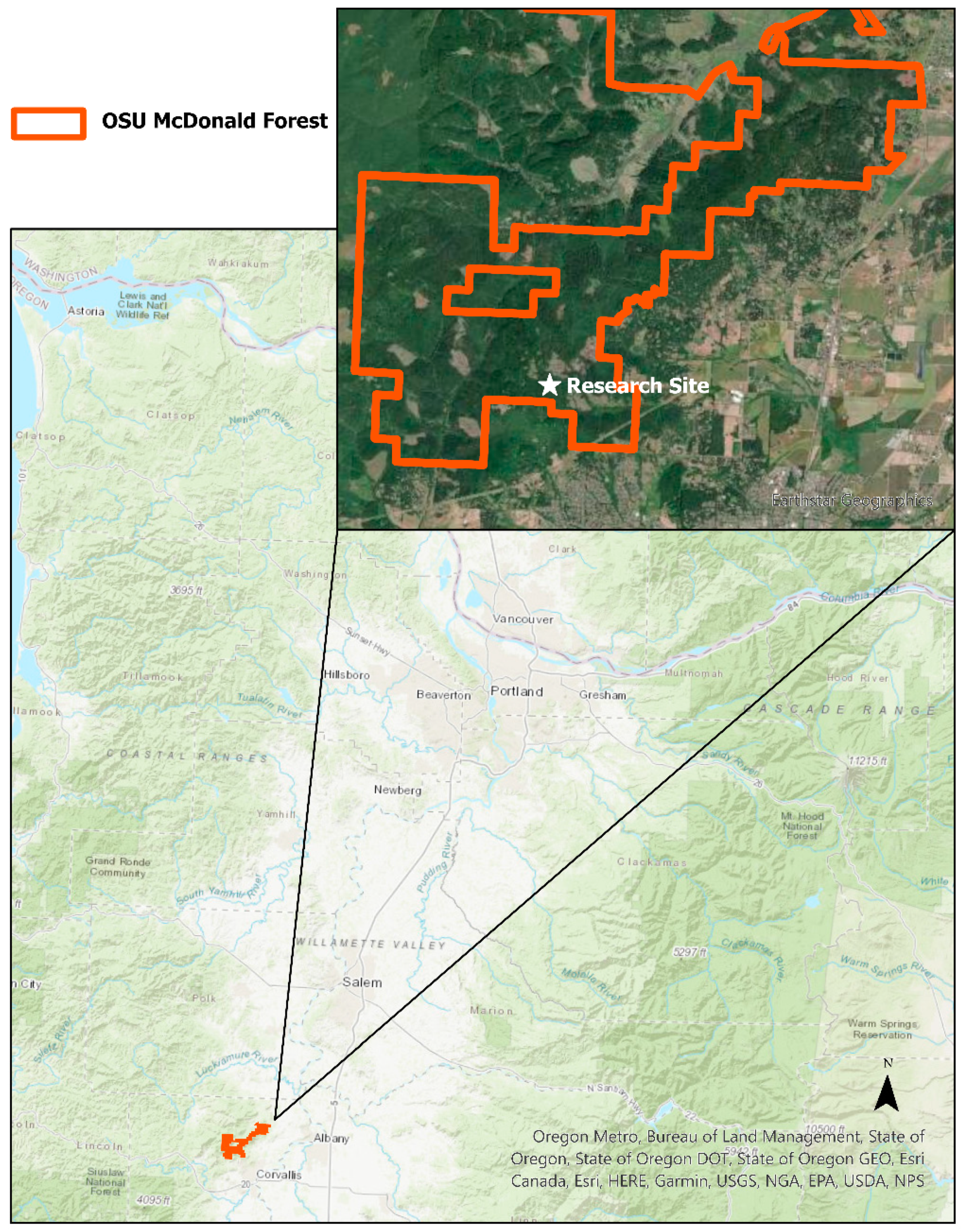
2.1. Study Area
2.2. Data Collection
2.2.1. Field Inventory for Visual Assessment of Damages
2.2.2. Photogrammetric Imagery and Point Cloud Generation
- Focal length: 4 mm;
- Maximum aperture: 153;
- 35 mm focal length: 26;
- Flash: no flash;
- Exposure time: automatic, variable;
- ISO speed: automatic, variable;
- File type: .jpg, converted to tiff.
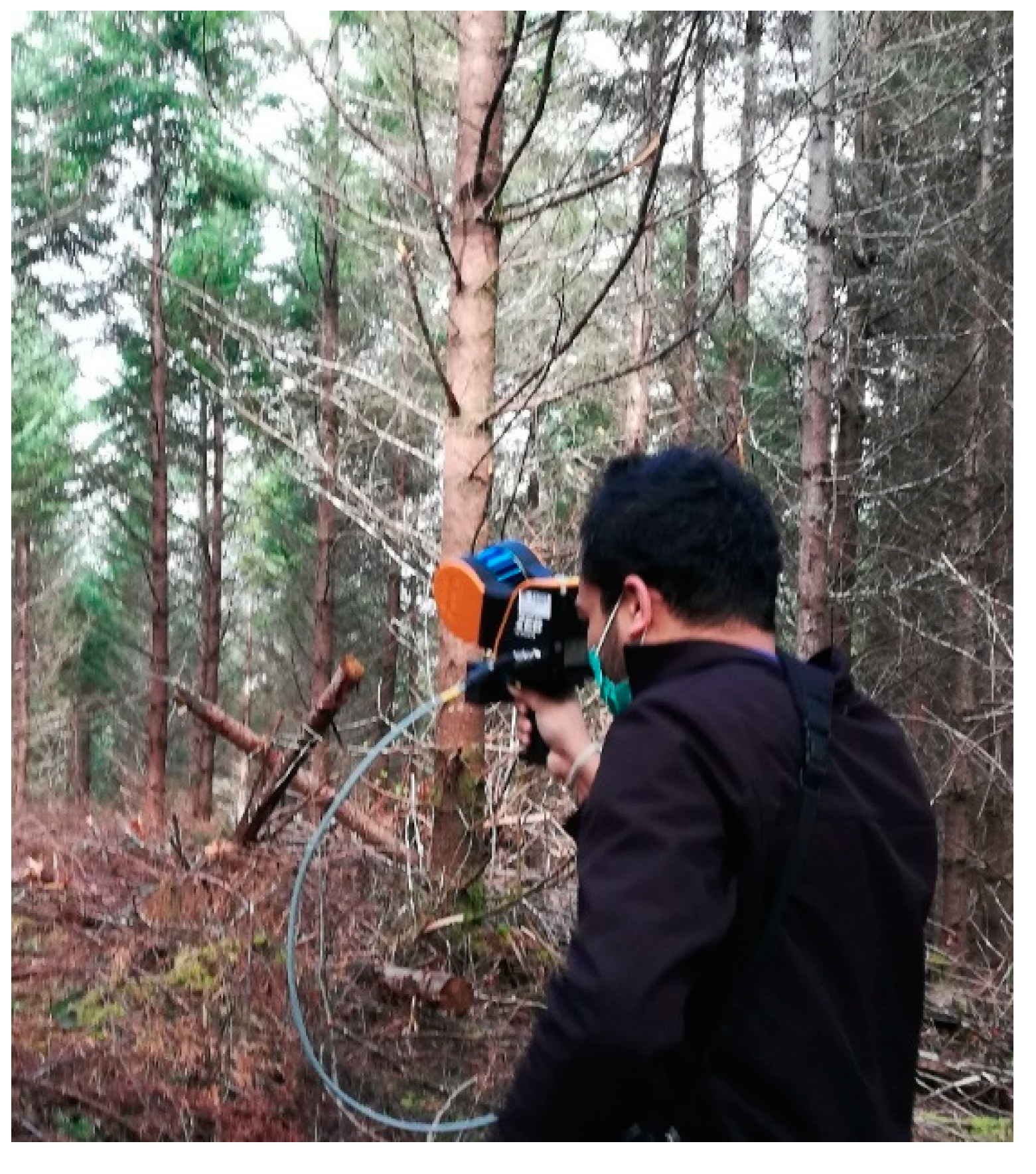
2.2.3. Handheld Lidar
2.3. Point Cloud Measurements
2.4. Data Analysis
- y = subject’s response vector (observed);
- X = fixed effects design matrix (known);
- β = fixed effects parameter vector (unknown);
- Z = random effects design matrix (known);
- γ = random effects parameter vector (unknown);
- ϵ = vector of independent (Gaussian), random errors (unobserved).
3. Results
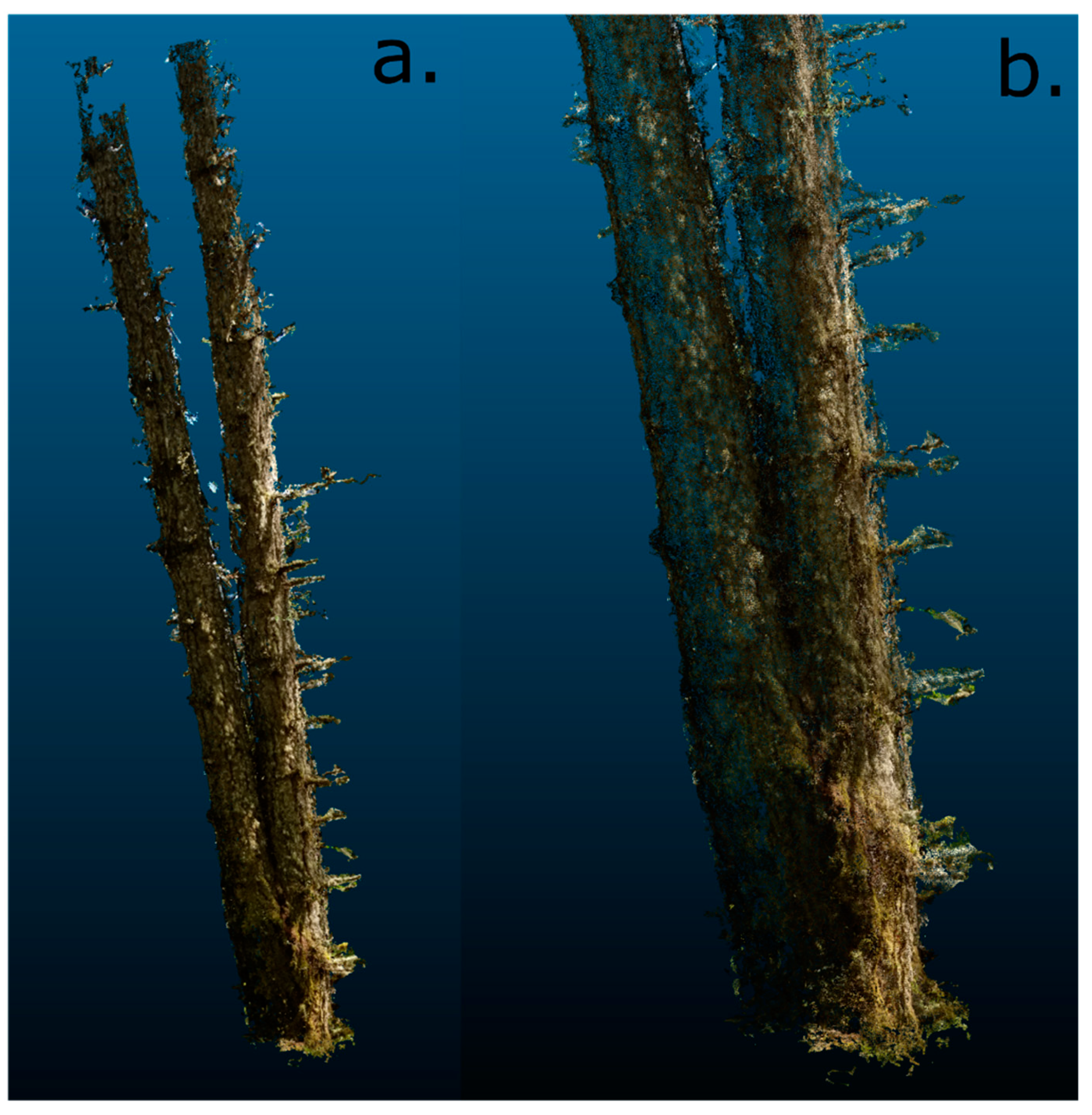
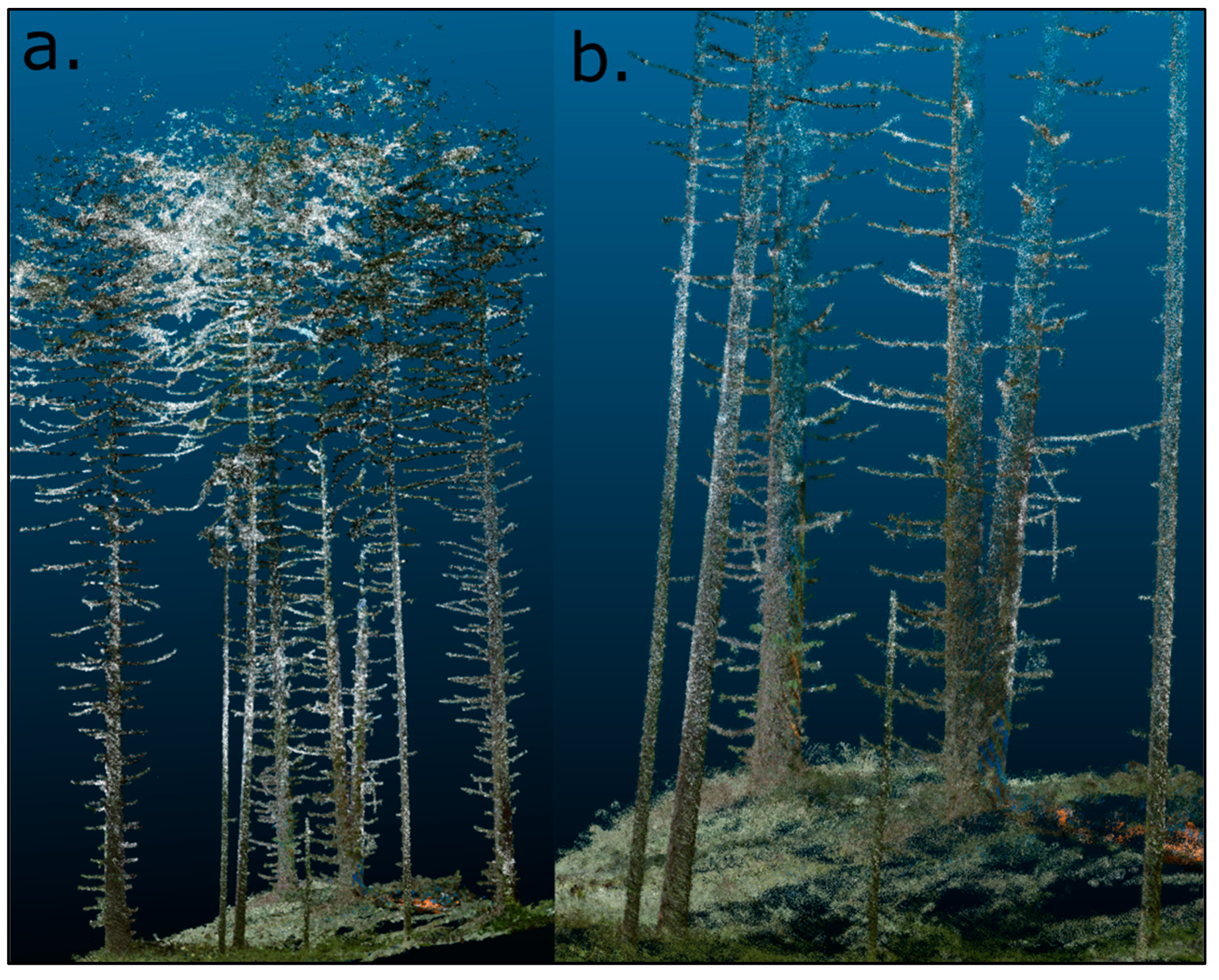
3.1. Point Clouds
3.2. Damage Count and Length
4. Discussion
4.1. Damage Count
4.2. Damage Length
5. Conclusions
Author Contributions
Funding
Data Availability Statement
Acknowledgments
Conflicts of Interest
References
- Natural Resources Conservation Service. Forestry Technical Note No. FOR-1: Forest Inventory Methods; USDA: Washington, DC, USA, 2018.
- Bragg, D.C. An improved tree height measurement technique tested on mature southern pines. South. J. Appl. For. 2008, 32, 38–43. [Google Scholar] [CrossRef] [Green Version]
- Kitahara, F.; Mizoue, N.; Yoshida, S. Effects of training for inexperienced surveyors on data quality of tree diameter and height measurements. Silva Fenn. 2010, 44, 657–667. [Google Scholar] [CrossRef] [Green Version]
- Donager, J.J.; Meador, A.J.S.; Blackburn, R.C. Adjudicating perspectives on forest structure: How do airborne, terrestrial, and mobile lidar-derived estimates compare? Remote Sens. 2021, 13, 2297. [Google Scholar] [CrossRef]
- Gollob, C.; Ritter, T.; Nothdurft, A. Forest inventory with long range and high-speed personal laser scanning (PLS) and simultaneous localization and mapping (SLAM) Technology. Remote Sens. 2020, 12, 1509. [Google Scholar] [CrossRef]
- Hyyppä, E.; Yu, X.; Kaartinen, H.; Hakala, T.; Kukko, A.; Vastaranta, M.; Hyyppä, J. Comparison of backpack, handheld, under-canopy UAV, and above-Canopy UAV laser scanning for field reference data collection in boreal forests. Remote Sens. 2020, 12, 3327. [Google Scholar] [CrossRef]
- GeoSLAM. ZEB Horizon. Available online: https://geoslam.com/solutions/zeb-horizon (accessed on 10 October 2021).
- Fang, R.; Strimbu, B.M. Stem measurements and taper modeling using photogrammetric point clouds. Remote Sens. 2017, 9, 716. [Google Scholar] [CrossRef] [Green Version]
- Iglhaut, J.; Cabo, C.; Puliti, S.; Piermattei, L.; O’Connor, J.; Rosette, J. Structure from Motion photogrammetry in forestry: A review. Curr. For. Rep. 2019, 5, 155–168. [Google Scholar] [CrossRef] [Green Version]
- Liang, X.; Jaakkola, A.; Wang, Y.; Hyyppä, J.; Honkavaara, E.; Liu, L.; Kaartinen, H. The use of a hand-held camera for individual tree 3D mapping in forest sample plots. Remote Sens. 2014, 6, 6587–6603. [Google Scholar] [CrossRef] [Green Version]
- Mikita, T.; Janata, P.; Surový, P. Forest stand inventory based on combined aerial and terrestrial close-range photogrammetry. Forests 2016, 7, 165. [Google Scholar] [CrossRef] [Green Version]
- Surový, P.; Yoshimoto, A.; Panagiotidis, D. Accuracy of reconstruction of the tree stem surface using terrestrial close-range photogrammetry. Remote Sens. 2016, 8, 123. [Google Scholar] [CrossRef] [Green Version]
- Liu, J.; Feng, Z.; Yang, L.; Mannan, A.; Khan, T.; Zhao, Z.; Cheng, Z. Extraction of sample plot parameters from 3D point cloud reconstruction based on combined RTK and CCD continuous photography. Remote Sens. 2018, 10, 1299. [Google Scholar] [CrossRef] [Green Version]
- Mokroš, M.; Liang, X.; Surový, P.; Valent, P.; Čerňava, J.; Chudý, F.; Tunák, D.; Saloň, Š.; Merganič, J. Evaluation of close-range photogrammetry image collection methods for estimating tree diameters. ISPRS Int. J. Geo-Inform. 2018, 7, 93. [Google Scholar] [CrossRef] [Green Version]
- Piermattei, L.; Karel, W.; Wang, D.; Wieser, M.; Mokroš, M.; Surový, P.; Koreň, M.; Tomaštík, J.; Pfeifer, N.; Hollaus, M. Terrestrial Structure from Motion photogrammetry for deriving forest inventory data. Remote Sens. 2018, 11, 950. [Google Scholar] [CrossRef] [Green Version]
- Raumonen, P.; Greco, R.; Persia, M.; Tartarino, P.; Marzulli, M.I. Estimating tree stem diameters and volume from smartphone photogrammetric point clouds. Forestry 2020, 93, 411–429. [Google Scholar]
- Bell, J.F.; Dilworth, J.R. Log Scaling and Timber Cruising; John Bell & Associates, Inc.: Corvallis, OR, USA, 2007; 397p. [Google Scholar]
- Nguyen, V.-T.; Constant, T.; Kerautret, B.; Debled-Rennesson, I.; Colin, F. A machine-learning approach for classifying defects on tree trunks using terrestrial LiDAR. Comput. Electron. Agric. 2020, 171, 105332. [Google Scholar] [CrossRef]
- Stangle, S.M.; Brochert, F.; Kretschmer, U.; Spiecker, H.; Sauter, U.H. Clear wood content in standing trees predicted from branch scar measurements with terrestrial LiDAR and verified with X-ray computed tomography. Can. J. For. Res. 2014, 44, 145–153. [Google Scholar] [CrossRef]
- Mengesha, T.; Hawkins, M.; Tarleton, M.; Nieuwenhuis, M. Stem quality assessment using terrestrial laser scanning technology: A case study of ash trees with a range of defects in two stands in Ireland. Scand. J. For. Res. 2015, 30, 605–616. [Google Scholar] [CrossRef]
- Garms, C.G.; Strimbu, B.M. Impact of stem lean on estimation of Douglas-fir (Pseudotsuga menziesii) diameter and volume using mobile lidar scans. Can. J. For. Res. 2021, 51, 1117–1130. [Google Scholar] [CrossRef]
- Bauwens, S.; Bartholomeus, H.; Calders, K.; Lejeune, P. Forest inventory with terrestrial LiDAR: A comparison of static and hand-held mobile laser scanning. Forests 2016, 7, 127. [Google Scholar] [CrossRef] [Green Version]
- Jurjević, L.; Liang, X.; Gašparović, M.; Balenović, I. Is field-measured tree height as reliable as believed—Part II, A comparison study of tree height estimates from conventional field measurement and low-cost close-range remote sensing in a deciduous forest. ISPRS J. Photogramm. Remote Sens. 2020, 169, 227–241. [Google Scholar] [CrossRef]
- Panagiotidis, D.; Surový, P.; Kuželka, K. Accuracy of Structure from Motion models in comparison with terrestrial laser scanner for the analysis of DBH and height influence on error behaviour. J. For. Sci. 2016, 62, 357–365. [Google Scholar] [CrossRef] [Green Version]
- Akpo, H.A.; Atindogbé, G.; Obiakara, M.C.; Adjinanoukon, A.B.; Gbedolo, M.; Lejeune, P.; Fonton, N.H. Image data acquisition for estimating individual trees metrics: Closer is better. Forests 2020, 11, 121. [Google Scholar] [CrossRef] [Green Version]
- Huang, H.; Zhang, H.; Chen, C.; Tang, L. Three-dimensional digitization of the arid land plant Haloxylon ammodendron using a consumer-grade camera. Ecol. Evol. 2018, 8, 5891–5899. [Google Scholar] [CrossRef] [PubMed]
- Lange, I.D.; Perry, C.T. A quick, easy and non-invasive method to quantify coral growth rates using photogrammetry and 3D model comparisons. Methods Ecol. Evol. 2020, 11, 714–726. [Google Scholar] [CrossRef]
- Krisanski, S.; Taskhiri, M.S.; Turner, P. Enhancing methodsw for under-canopy unmanned aircraft systems based photogrammetry in complex forests for tree diameter measurement. Remote Sens. 2020, 12, 1652. [Google Scholar] [CrossRef]


| Damage Code One | General Damage | Damage Code Two | Specific Damage | Location Code | Damage Location |
|---|---|---|---|---|---|
| 0 | No Damage | 0 | No Damage | 1 | Bottom Third |
| 2 | Middle Third | ||||
| 1 | Unknown | 0 | Unknown | 3 | Top Third |
| 2 | Mechanical | 1 | Fire | ||
| Logging | |||||
| 3 | Chemical | 1 | Herbicide | ||
| 4 | Disease | 0 | Unknown | ||
| 1 | Mistletoe | ||||
| 2 | Needle rusts | ||||
| 3 | Stem decay | ||||
| 4 | Stem rusts | ||||
| 5 | Stem chancre | ||||
| 5 | Insects | 1 | Defoliators | ||
| 2 | Bark beetles | ||||
| 3 | Sucking insects | ||||
| 4 | Pitch moths | ||||
| 6 | Animal | 1 | Deer or elk | ||
| 2 | Bear | ||||
| 3 | Livestock | ||||
| 4 | Porcupine | ||||
| 5 | Mountain beaver | ||||
| 7 | Weather | 1 | Windthrow | ||
| 2 | Snow, ice, freeze | ||||
| 3 | Drought | ||||
| 4 | Lightning | ||||
| 5 | Flooding | ||||
| 8 | Suppression | 0 | Suppression | ||
| 9 | Physical | 0 | Butt swell | ||
| 1 | Broken top | ||||
| 2 | Dead top | ||||
| 3 | Multiple tops | ||||
| 4 | Forked tree | ||||
| 5 | Leaning tree | ||||
| 6 | Crook or sweep | ||||
| 7 | Seam or crack | ||||
| 8 | Spike knot | ||||
| 9 | Other |
| Measurement | Model | Type of Measurement | Units | Methodology |
|---|---|---|---|---|
| DBH | LiDAR | Linear | Meter |
|
| Model Height | SfM | Linear | Meter |
|
| Damage Type | SfM, LiDAR | Qualitative | None |
|
| Damage Location | SfM, LiDAR | Linear | None |
|
| Damage Length | SfM, LiDAR | Linear | Meter |
|
| Damage Count | SfM, LiDAR | Qualitative | None |
|
| Plot | RMSE (cm) | Bias (cm) |
|---|---|---|
| 1 | 1.89 | 0.79 |
| 2 | 1.00 | −0.60 |
| 3 | 4.04 | 0.91 |
| Plot | Handheld LiDAR Point Cloud Density (Mean Points per m2) | Handheld LiDAR Point Cloud Density (Mean Points per Tree) | SfM Point Cloud Density (Mean Points per Tree) |
|---|---|---|---|
| 1 | 7033 | 295,805 | 1,269,262 |
| 2 | 11,425 | 478,417 | 1,602,534 |
| 3 | 10,212 | 710,130 | 1,455,675 |
| Type 3 Tests of Fixed Effects | Least Squares Means | |||
|---|---|---|---|---|
| Effect | p-Value | Effect | Estimate | Standard Error 1 |
| Method | 0.003 | Visual | 1.62 | 0.21 (a) |
| LiDAR | 0.93 | 0.21 (b) | ||
| PPC | 0.93 | 0.21 (b) | ||
| Plot | 0.009 | Plot 1 | 1.39 | 0.20 (a) |
| Plot 2 | 1.42 | 0.21 (a) | ||
| Plot 3 | 0.66 | 0.26 (b) | ||
| Type 3 Tests of Fixed Effects | Least Squares Means | |||
|---|---|---|---|---|
| Effect | p-Value | Effect 1 | Estimate | Standard Error 2 |
| Method | 0.584 | Visual | 2.69 | 0.34 |
| LiDAR | 2.30 | 0.41 | ||
| PPC | 2.49 | 0.38 | ||
| Plot | 0.896 | Plot 1 | 2.59 | 0.33 |
| Plot 2 | 2.43 | 0.33 | ||
| Plot 3 | 2.47 | 0.52 | ||
| Damage Code | <0.0001 | 43 | 6.21 | 0.81 (a) |
| 45 | 1.82 | 0.44 (bc) | ||
| 52 | 1.60 | 1.56 (abc) | ||
| 90 | 1.83 | 0.70 (abc) | ||
| 91 | 1.04 | 0.79 (bc) | ||
| 93 | 8.61 | 1.56 (ab) | ||
| 94 | 1.56 | 0.40 (bc) | ||
| 95 | 1.60 | 1.57 (abc) | ||
| 96 | 1.31 | 0.30 (c) | ||
| 97 | 2.13 | 0.80 (abc) | ||
| 98 | 0.91 | 0.35 (c) | ||
| 99 | 1.34 | 1.10 (abc) | ||
Publisher’s Note: MDPI stays neutral with regard to jurisdictional claims in published maps and institutional affiliations. |
© 2022 by the authors. Licensee MDPI, Basel, Switzerland. This article is an open access article distributed under the terms and conditions of the Creative Commons Attribution (CC BY) license (https://creativecommons.org/licenses/by/4.0/).
Share and Cite
Morgan, C.J.; Powers, M.; Strimbu, B.M. Estimating Tree Defects with Point Clouds Developed from Active and Passive Sensors. Remote Sens. 2022, 14, 1938. https://doi.org/10.3390/rs14081938
Morgan CJ, Powers M, Strimbu BM. Estimating Tree Defects with Point Clouds Developed from Active and Passive Sensors. Remote Sensing. 2022; 14(8):1938. https://doi.org/10.3390/rs14081938
Chicago/Turabian StyleMorgan, Carli J., Matthew Powers, and Bogdan M. Strimbu. 2022. "Estimating Tree Defects with Point Clouds Developed from Active and Passive Sensors" Remote Sensing 14, no. 8: 1938. https://doi.org/10.3390/rs14081938
APA StyleMorgan, C. J., Powers, M., & Strimbu, B. M. (2022). Estimating Tree Defects with Point Clouds Developed from Active and Passive Sensors. Remote Sensing, 14(8), 1938. https://doi.org/10.3390/rs14081938