Abstract
The decline in biodiversity in Mediterranean-type ecosystems (MTEs) and other shrublands underscores the importance of understanding the trends in species loss through consistent vegetation mapping over broad spatial and temporal ranges, which is increasingly accomplished with optical remote sensing (imaging spectroscopy). Airborne missions planned by the National Aeronautics and Space Administration (NASA) and other groups (e.g., US National Ecological Observatory Network, NEON) are essential for improving high-quality maps of vegetation and plant species. These surveys require robust and efficient ground calibration/validation data; however, barriers to ground-data collection exist, such as steep terrain, which is a common feature of Mediterranean-type ecosystems. We developed and tested a method for rapidly collecting ground-truth data for shrubland plant communities across steep topographic gradients in southern California. Our method utilizes semi-aerial photos taken with a high-resolution digital camera mounted on a telescoping pole to capture groundcover, and a point-intercept image-classification program (Photogrid) that allows efficient sub-sampling of field images to derive vegetation percent-cover estimates while reducing human bias. Here, we assessed the quality of data collection using the image-based method compared to a traditional point-intercept ground survey and performed time trials to compare the efficiency of various survey efforts. The results showed no significant difference in estimates of percent cover and Simpson’s diversity derived from the point-intercept and those derived using the image-based method; however, there was lower correspondence in estimates of species richness and evenness. The image-based method was overall more efficient than the point-intercept surveys, reducing the total survey time by 13 to 46 min per plot depending on sampling effort. The difference in survey time between the two methods became increasingly greater when the vegetation height was above 1 m. Due to the high correspondence between estimates of species percent cover derived from the image-based compared to the point-intercept method, we recommend this type of survey for the verification of remote-sensing datasets featuring percent cover of individual species or closely related plant groups, for use in classifying UAS imagery, and especially for use in MTEs that have steep, rugged terrain and other situations such as tall, dense-growing shrubs where traditional field methods are dangerous or burdensome.
Keywords:
biodiversity; imaging spectroscopy; field protocol; validation; calibration; shrubland; vegetation 1. Introduction
Mediterranean-type ecosystems (MTEs) are biodiversity hotspots, accounting for almost 20% of the world’s species in 5% of its area [1,2]. Heterogeneity in climate, topography, and fire regimes contributes to these high levels of species diversity [3,4,5]; however, climate change, frequent fire, urbanization, and non-native plant invasions are threatening the biodiversity of MTEs, leading to species extinctions as well as rapid changes in vegetation cover [2,4,6]. Therefore, it is essential to understand the trends in species loss and monitor changes in biodiversity [7]. This requires the capacity to consistently monitor occurrences of species or assemblages over broad spatial and temporal ranges, which is increasingly accomplished with advanced optical remote-sensing technologies, such as imaging spectroscopy [7,8,9,10,11,12].
Imaging spectroscopy of multispectral or hyperspectral remote-sensing data is a rapidly expanding method used in ecological and conservation applications. In the context of biodiversity monitoring, imaging spectroscopy relates the spectral properties of an area with other biodiversity metrics such as species identity and diversity, functional traits, or other variables such as photosynthetic vegetation, nitrogen content, etc. [12,13,14,15]. Analyses have been broadly applied across ecosystems, including forest, dryland, marine, and urban ecosystems with increasing emphasis on the identification of individual species and/or mapping plant species diversity at landscape scales [13,14,15].
The expanding use of remote sensing and imaging spectroscopy to estimate metrics of biodiversity requires robust verification and validation protocols that generate measures consistent with traditional ground-survey methods. This need is intensified by forthcoming spaceborne spectral missions, such as NASA’s Surface Biology and Geology mission (SBG) and other related missions in Europe and Japan [16,17]. However, validation will be challenging for spaceborne data given the extent and volume of measurements that will be needed to accommodate global satellite missions. To quantify how remote measurements relate to traditional metrics of biodiversity, it is important to understand how they scale across different ecosystems, including those that are under-studied due to limited access.
While topographic heterogeneity contributes to biodiversity in MTEs, it also creates barriers to their study due to large regions that are too steep for traditional field surveys. Studies of these regions either lack data or rely heavily on visual estimation (e.g., [18,19,20]). Furthermore, much of the protected land in MTEs occurs in steep, moderate- to high-elevation regions, which are unsuitable for development, making the study of these areas even more important for understanding trends in biodiversity [6]. While all remote-sensing studies include some type of mechanism to compare algorithmic results to reality, often the baseline condition is derived from satellite imagery or potentially outdated ground surveys, which were not always performed with the original purpose of being used to validate remote-sensing predictions [21]. Finally, the prospect of worldwide satellite-data collection intensifies the need for efficient, accurate ground-truthing methods that can be applied in a variety of landscape settings while maintaining accuracy among users.
Here, we sought to develop a field protocol appropriate for calibrating and validating vegetation-mapping algorithms from optical remote-sensing data, with a focus on methods that can be rapidly implemented in the rugged shrubland ecosystems that are characteristic of MTEs. Because optical remote sensing primarily characterizes the top of the canopy of vegetation, our method prioritizes the enumeration of species composition from semi-aerial photos taken above the canopy [22,23,24]. This method has been successfully used to document classes of vegetation cover in rangelands, but has less often been applied to identifying species [25,26]. Vegetation-cover surveys were performed for 83 45-m × 45-m plots of mostly shrubland plant communities in the southern California San Gabriel Mountains. The pictures were analyzed using a classification procedure in which species were identified on a grid superimposed on the pictures [27,28]. We evaluated the accuracy and efficiency of the method in both flat and steep terrain, and discuss the tradeoffs between more traditional vegetation-cover surveys and this method at different sampling efforts and for estimating various metrics of plant species diversity. We present this approach as a viable alternative for intensive surveys in shrublands, especially in settings where traditional surveys are impractical due to difficulty traversing steep terrain or other conditions.
2. Methods
2.1. Study-Site Description
Data collection occurred in two post-burn areas in the Angeles National Forest in southern California, with elevations ranging from less than 400 m to over 1300 m above sea level (Figure 1). The mean (SE) slope of our study area was 27.3 (1.2) percent; however, 46 of our study plots (nearly half of the total) had an average slope value greater than 30 percent, and 14 plots had slopes greater than 40 percent. The Copper and Sayre fires occurred in 2002 and 2008, respectively, both at high intensities, burning a collective 25,000 acres. In the following years, there has been re-growth of the predominantly montane chaparral and coastal sage scrub vegetation types, as well as the establishment of non-native invasive forbs and grasses. Information on the amount of area revegetated to native and non-native vegetation, and the composition of that vegetation, has been limited by the notably steep and rugged terrain of the San Gabriel Mountains.
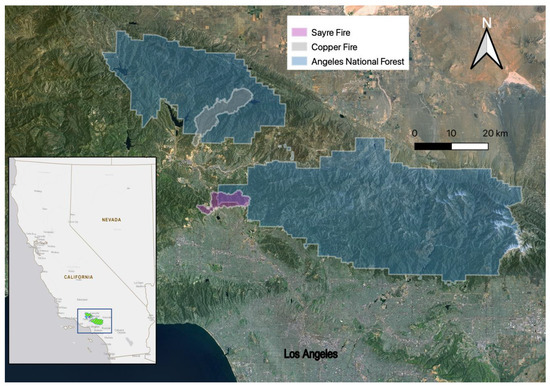
Figure 1.
Map of the study area in the Angeles National Forest (green), Los Angeles County, CA, USA. The Copper and Sayre fires burned approximately 25,000 acres between 2002 and 2008.
2.2. Field Plot Selection
In the spring and summer of 2018, the cover of all plant species was recorded from 83 field plots (43 within the Copper fire and 40 within the Sayre fire) consisting of low-and mid-statured vegetation (mainly shrubs and herbaceous species). A LiDAR digital elevation model was used to quantify the area of the study site falling within distinct topographic zones of elevation, slope, and aspect, and to ensure that the survey plots sampled a similar proportion of attributes as the survey area itself (Supplementary Materials S1: Figure S1) [29].
Each survey plot was 45 m × 45 m and was delineated in the field based upon the uniformity of vegetation, slope, and aspect. We aimed to survey individual plots that were representative of a single cover class (plant species, ground cover, etc.) or vegetation community/alliance. We similarly aimed to survey plots having uniform slope and aspect within the plot boundary.
Plots were classified as either “steep” or “flat” based on their average percent slope. “Steep” plots (having slopes greater than 10 percent, 69 plots total) were surveyed using a “Steep Protocol” to optimize efficiency and safety of surveyors, whereas “flat” plots (with an average slope less than 10 percent, 14 plots total) were surveyed with the “Flat Protocol” (both described below and pictured in Figure 2).

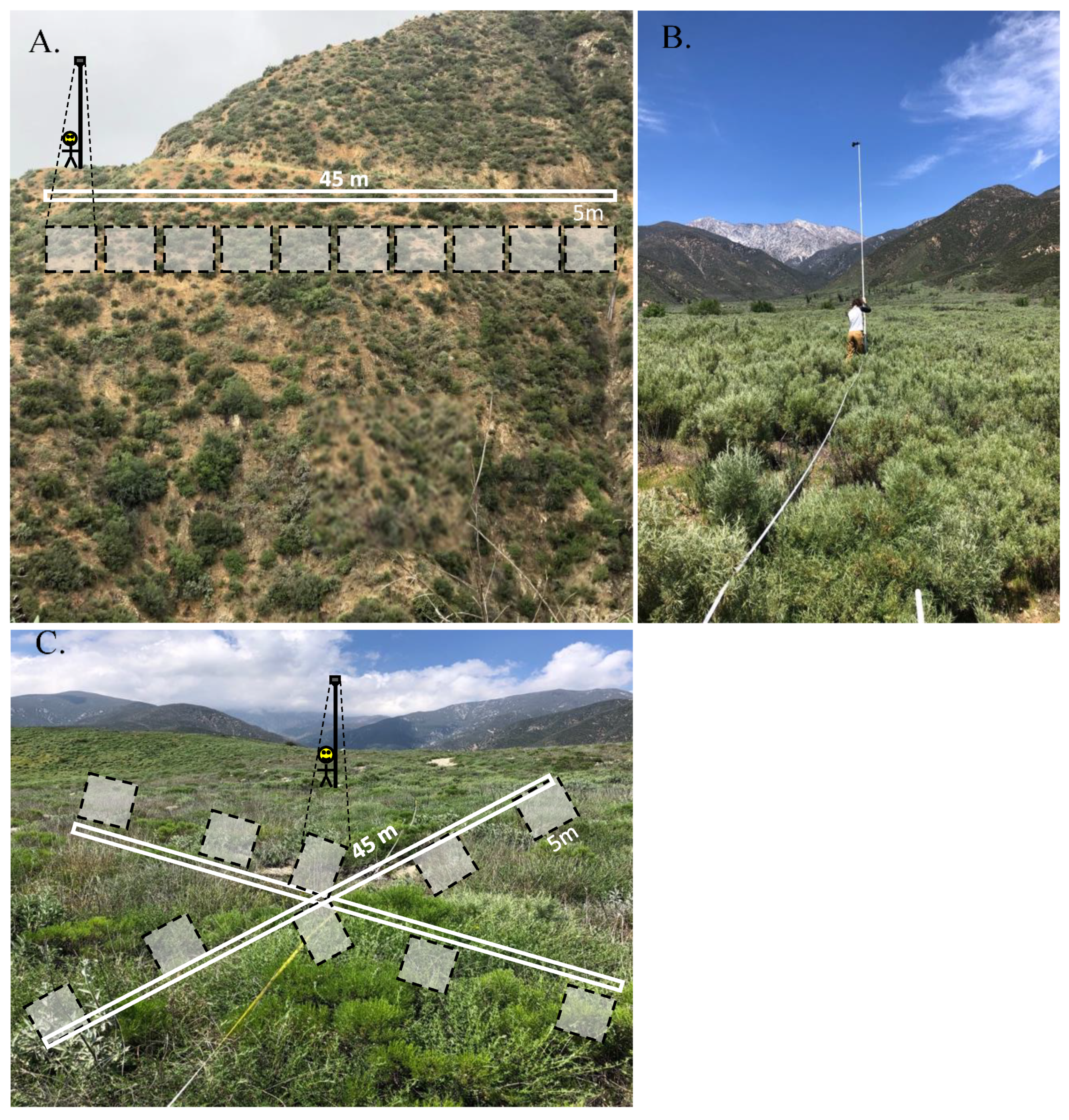
Figure 2.
Diagram of photo-survey method for (A) steep plots: surveyor walks along a 45-m transect taking 10 5-m × 5-m photos (grey boxes) of the plot below, (B) a field crew member taking photos with camera attached to a pole extended 5 m, and (C) diagram of photo survey for flat plots: surveyor walks along two crossed 45-m transects taking 10 5-m × 5-m photos from above.
2.3. Image-Based Method: Field Sampling
Photogrid (Liu, Singh and Townsend, https://github.com/EnSpec/PhotoGrid) is an open-source Python program that was developed for users to classify plant species from field photos using an image-based point-intercept sampling schema. The program superimposes a user-defined grid over a photograph of a field plot, and an analyst manually identifies the species present at each crosshair. From this, users can calculate standard metrics of species composition and diversity, such as percent cover by species or species richness. Sampling of vegetation using Photogrid requires the use of a sufficient-resolution camera operated at a low enough altitude to enable species identification. Here, we used a camera attached to a 6 m telescoping fiberglass pole (Wonder Pole, American Flag & Banner Company, Salem, OR, USA).
To survey plots with steep slopes we followed the “Steep Protocol.” A 45-m transect was laid along a ridgeline (generally a roadside or trail) and overhead photos were taken looking downslope along the transect using a Sony Alpha 5100 digital camera (16–50 mm lens, 23.5 × 15.6 mm CMOS sensor with 6.65 MP/cm2 pixel density) mounted to the fiberglass pole. The pole was extended to the appropriate height (generally 5–6 m) per ground-slope angle to capture an approximately 5-m × 5-m area within each photo frame, which was verified by placing a meter stick on the ground in the photo area for scaling (Figure 2A,B). The camera was set to automatic focus and was controlled wirelessly via the PlayMemories Mobile application [30]. We set the shutter speed and aperture settings each day depending on the light conditions (e.g., full sun, clouds, etc); although few adjustments were needed during our surveys. The PlayMemories application also allows for adjusting the aperture and shutter speed remotely if conditions are variable while taking the photos. Photos were taken every 5 m along the transect for a total of 10 photos per plot.
The “Flat Protocol” was used for plots surveyed in less-frequently occurring flat terrain. For these plots, two bisecting 45-m transects were laid out at 90-degree angles to each other and 10 5-m × 5-m ground photos were taken from above with the camera set-up (Figure 2C).
When using both Steep and Flat protocols, the area covered by the photos was also surveyed by experienced botanists to compile a complete plant census from ground surveys. An individual recorded all observable plant species by walking along the transect and broadly classified their percent coverage, as well as that of other cover classes such as bare ground and leaf litter. This individual also took notes on important identifying features (such as phenology and coloration of vegetation) and annotated a set of photos in the field to assist analysts back in the lab with species identification (Figure 3A). Static location points were taken along each survey transect with a Trimble R10 GNSS system to determine precise geographic locations of surveys for referencing with airborne imagery.

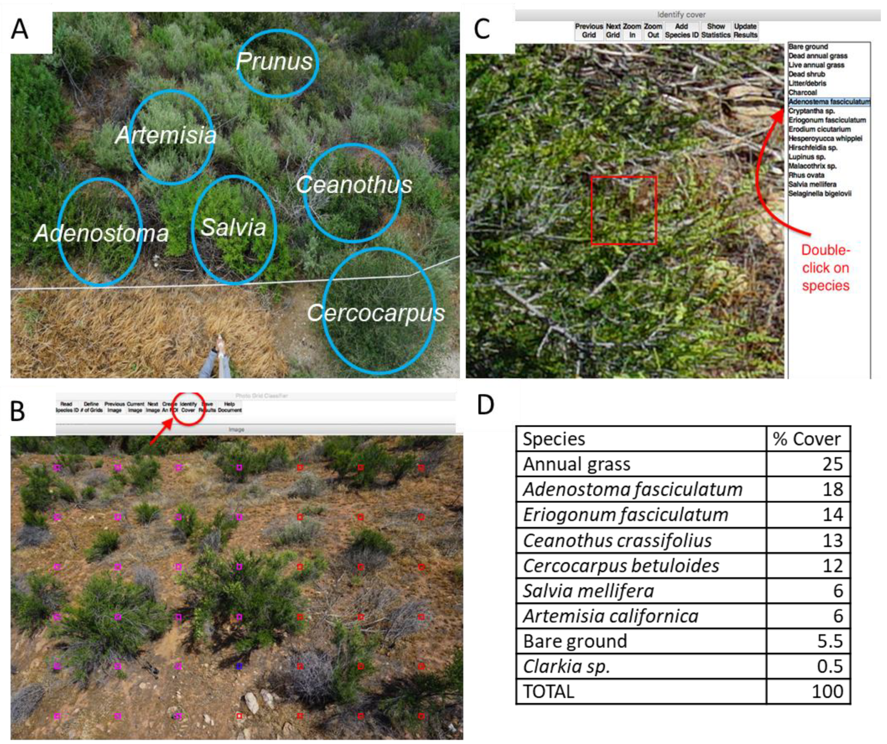
Figure 3.
Photogrid classification process: (A) in the field, aboveground photos were marked with a smartphone app to aid with later species ID; (B) back in the lab, photos were uploaded into the Photogrid classifier program and number of gridpoints per photo (generally 42) were chosen, which instructs the program to populate each photo with gridpoints to classify; (C) for each gridpoint, the user must select the dominant species/cover class within that cell from a pre-entered list; (D) after completing classification for all ten plot photos, a table is generated with percent cover of each class identified, out of 100% (Annual Grass was a composite category that included annual grass species that could not be distinguished in the photos such as Bromus spp., Avena spp., etc.).
2.4. Image-Based Method: Photo Analysis
Photogrid enables a systematic approach to classifying cover within photos to avoid human bias. For each 5-m × 5-m ground plot photo, we specified a grid of six rows and seven columns, totaling 42 sampling points per photo (Figure 3B) and 420 points per 10-photo plot. In Photogrid, each gridpoint is enclosed by a solid box on the screen; the user clicks on each box and is able to zoom in or out until they can classify the dominant species or cover class within the box and select it from a corresponding list compiled from all species and cover classes that were surveyed in the field within that particular plot (Figure 3C). Cover classes were used to accommodate the identification of bare ground, as well as a few taxa that were identifiable to genus or family from photographs, but not to species (e.g., annual grasses which included annual grass species such as Bromus spp., Avena spp., etc.). The program saves the user’s entry for each point and calculates percent cover for each species/class once all photos have been classified for a plot (Figure 3D).
2.5. Image-Based Method: Validation
The purpose of surveying the 83 plots in 2018 was to accurately and efficiently collect percent-cover data within the two fire zones. The image-based survey method allowed a large area to be surveyed over one field season, including many steep slopes that would have been impossible to survey using a traditional field-transect approach. Consequently, only species richness (based on surveys for species presence) could be precisely measured in each field plot in 2018; no other quantitative measures of species composition were taken using traditional ground surveys.
To compare the accuracy and efficiency of the image-based method with more traditional point-intercept field-transect surveys (henceforth “point-intercept method”), we employed a second field study in 2019 with an additional 16 plots that could be safely sampled with both the Photogrid and point-intercept methods. Due to a lack of level sites within the original study area, the 16 validation plots were located outside of the 2018 study sites, but within a nearby region of the San Gabriel Mountains with similar vegetation.
For the 2019 plots, species percent cover was estimated within a 45-m × 45-m plot. A 45-m baseline transect was established with seven perpendicular survey transects laid out evenly and extending 45 m from the baseline. Along these perpendicular transects, surveyors stopped every 1 m and recorded the tallest species or object at that exact point and in contact with a PVC touch pole with a diameter of 1.9 cm. If no standing object or vegetation was touching the pole at a single location, the ground cover class was recorded. A total of 315 survey points were recorded per plot, and the percentage of each species or object out of 315 points was calculated.
Each of the 16 plots was also surveyed by the image-based method, with 10 overhead photos taken per plot using the Flat Protocol as the plots had slopes less than 10 degrees. For the photos from these plots, we modified the Photogrid output to subsample the gridpoints to test how different levels of sampling effort affect the accuracy of estimates derived from Photogrid in comparison to the field-sampled point-intercept data. Twelve Photogrid configurations (henceforth referenced as configuration 1–12) were tested, each comprised of a different variation of rows, columns, and gridpoints surveyed per photo and entire plot (Table 1). Configuration 1 with 420 gridpoints had the highest sampling effort.

Table 1.
Average time to complete vegetation-cover survey by method (point-intercept vs. Photogrid) and by Photogrid configuration (1–12). Configuration 1 is the most detailed photo survey containing 420 gridpoints per plot, and configuration 12 is the least detailed with only 45 gridpoints. Point-intercept surveys (top row) have no Photogrid classification as percent cover was derived by a point-intercept survey in the field. All time data represent means from 13 field plots surveyed by both Photogrid and point-intercept methods in the spring of 2019 in various vegetation types.
Through experience we found that a three-person crew was optimal for surveying using either method, as adding additional people did not improve efficiency. Using a three-person crew, we kept detailed logs of time spent both in the field and on data processing out of the field for each plot and method. These data allowed us to compare the time spent per survey type and Photogrid configuration (Table 1). The time necessary to process the photos by each configuration was estimated based on the average time required to process photos by configuration 1, reduced proportionally based on the number of gridpoints in each configuration (Table 1).
2.6. Statistical Analysis
Because percent-cover data were not collected using traditional ground-sampling in the steep 2018 plots, only species richness was compared between field observations (Sfield) versus Photogrid survey (Sphoto), as well as by protocol (flat versus steep). In cases where a plant could only be identified to a genus or functional group, it was counted as one species (e.g., annual grasses). A paired t-test was used to compare Sfield with Sphoto across all plots in the 2018 dataset. To test the effect of protocol on the difference between Sphoto and Sfield, a linear model was used with Sphoto as the response variable, Sfield as a covariate, protocol (flat, steep) as a fixed factor, and the interaction between Sfield and protocol (Sphoto ~ Sfield + protocol + Sfield:protocol).
For the 2019 Photogrid method validation data, our goal was to assess the correspondence of the field and Photogrid surveys, as well as compare the correspondence of the 12 Photogrid configurations with field data. The following attributes were calculated for each plot using the Photogrid and point-intercept-method cover data: species richness (S), Simpson’s species diversity (1/D), and Simpson’s evenness (E). A linear model was used with the Photogrid attribute as the response variable (e.g., Sp), the field attribute as a covariate (e.g., Sp-i where “p-i” indicates the point-intercept method), Photogrid configuration as a fixed factor, and the interaction between the field attribute and configuration (e.g., Sp ~ Sp-i + configuration + Sp-i:configuration). A separate model was used to test each attribute. Percent cover was calculated for each species and cover class (% cover) in a plot; therefore, models testing % cover included a random factor for plot to account for multiple species measurements in each plot. Tukey tests were used to perform post-hoc comparisons for significant effects of configuration [31]. For all attributes, separate simple linear regression models and a correlation analysis were analyzed for each configuration to report the model coefficients by configuration. Simple linear regression models were used to analyze the relationship between % coverp using configuration one and % coverp-i for species and cover classes observed in more than 50% of the plots (9 or more plots).
For the 2019 surveys, time data were analyzed to assess the efficiency of each method and whether efficiency varied with the height of vegetation, e.g., comparing low grasses or shrubs with taller shrubs. Plots were categorized into one of three classes based on visual estimation of vegetation height: low (<1 m, 4 plots), mid (1 m to 1.5 m, 7 plots), and high (>1.5 m, 2 plots). The response variable of time to complete a plot survey was analyzed with a repeated measures linear mixed model. The model included method (Photogrid or point-intercept) and height class as fixed factors and the method × height class interaction term. For this repeated-measures model, the plot was treated as a random factor to account for two measures in each plot. All data were analyzed in R using the lme4 package [32,33].
3. Results
3.1. 2018 Large-Scale Survey
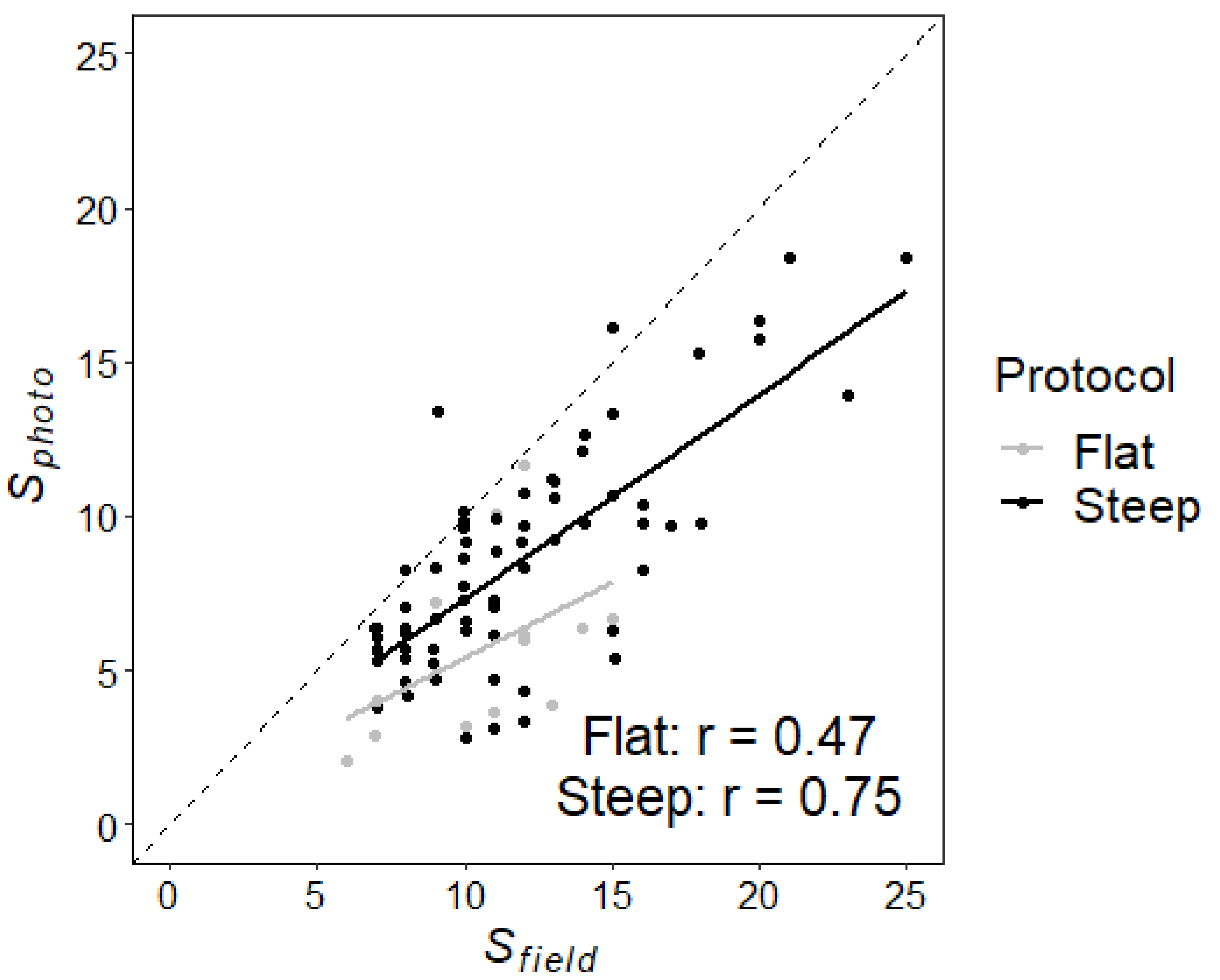
There was a significant effect of Sfield (F1,79 = 95.55, p < 0.0001) and protocol (flat or steep; F1,79 = 7.91, p = 0.006) on Sphoto, with no significant interaction (F1,79 = 0.47, p > 0.05). However, a disproportionate number of steep plots were surveyed relative to flat plots due to a lack of level terrain in the study area (Figure 4). On average, field surveys recorded 3.6 more species than the Photogrid method (paired t-test, T163 = 6.16, p < 0.001).

Figure 4.
Relationship between species richness of field observations (Sfield) and Photogrid surveys (Sphoto) for Flat and Steep protocols. Data are from 2018 field surveys including 69 steep (shown in black) and 14 flat plots (shown in grey). The dashed line is the one-to-one line. Results of a linear mixed-effects regression showed a significant effect of Sfield (F1,79 = 95.55, p < 0.0001) and protocol (F1,79 = 7.91, p = 0.006) on Sphoto, with no significant interaction (F1,79 = 0.47, p > 0.05). Pearson correlation coefficients between Sphoto and Sfield are shown.
3.2. 2019 Point-Intercept Validation Study: Accuracy
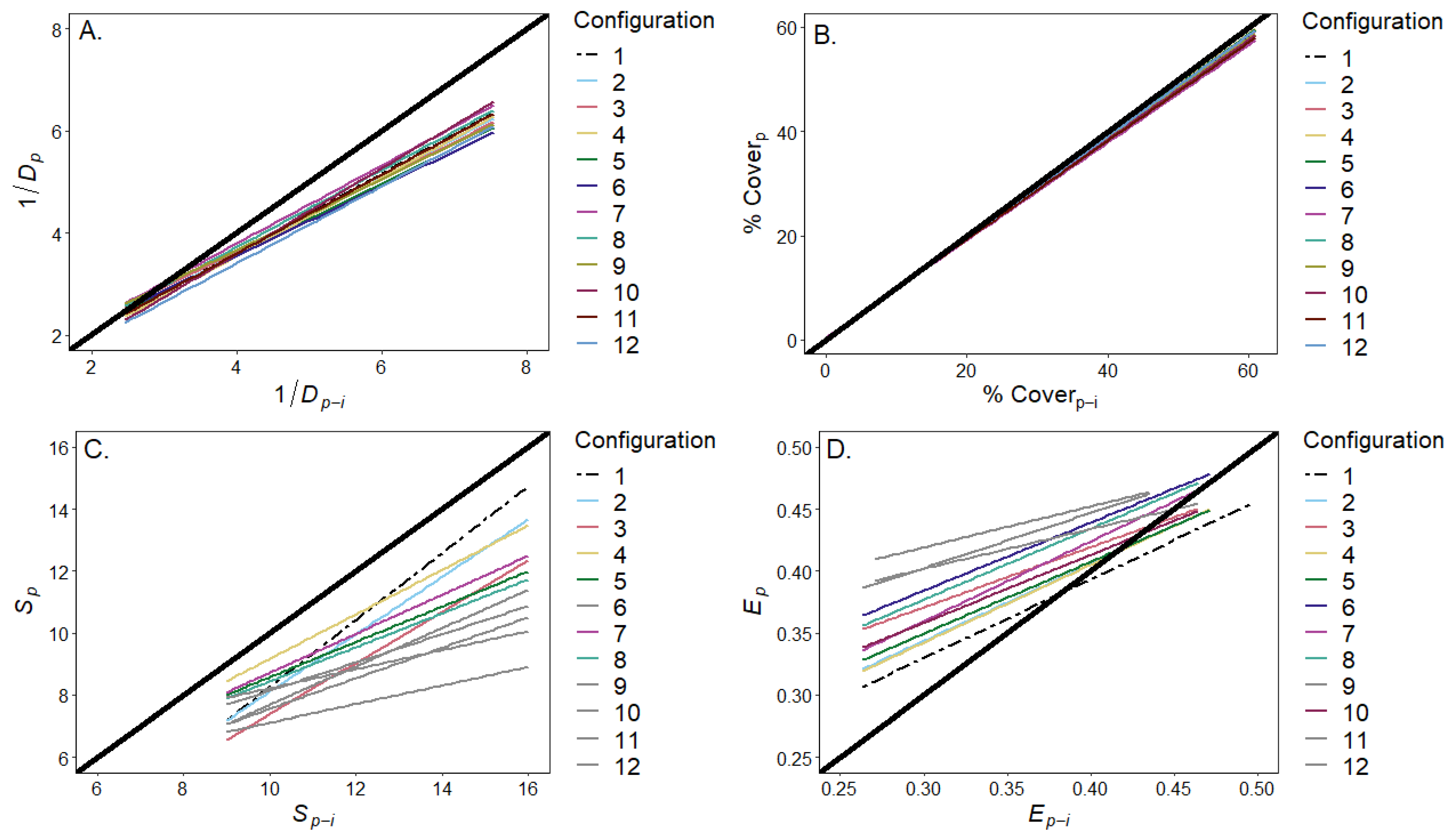
Species-diversity and percent-cover estimates were not significantly affected by Photogrid configuration. All 12 configurations produced similar results to each other for both metrics and there was no significant interaction between configuration and either attribute (Table 2; Figure 5A,B). However, 1/Dp was consistently less than 1/Dp-i across all configurations (Supplementary Materials S1: Table S1; Figure 5A). There was little deviation from the one-to-one relationship among the configurations for % cover (Supplementary Materials S1: Table S2; Figure 5B). The Pearson correlation coefficients between point-intercept estimates and those from Photogrid configuration 1 (the highest sampling effort) were 0.91 for 1/D and 0.93 for % cover (Supplementary Materials S1: Tables S2 and S3).
Table 2.
Test statistic (F), significance (p), and degrees of freedom are reported for each factor and interaction term for linear models for four vegetation metrics: % cover, species richness (S), Simpson’s species diversity (1/D), and Simpson’s evenness (E).

Figure 5.
Regressions between field (e.g., Sp-i) and Photogrid (e.g., Sp) vegetation metrics from the 2019 data, shown for the 12 Photogrid configurations of (A) Simpson’s species diversity (1/D); (B) % Cover; (C) species richness (S); and (D) Simpson’s evenness. The heavy black lines show the one-to-one relationship. Dashed lines represent the regression between Photogrid configuration 1 (highest sampling effort) and the field point-intercept method; colored lines are those configurations that did not produce significantly different results from configuration 1, and grey lines represent those that were significantly different than configuration 1, based on a Tukey HSD test. There was no significant difference among the configurations for 1/Dp or % Coverp. Five configurations produced significantly lower values for Sp, and three configurations produced significantly greater values for Ep when compared to configuration 1.
The relationships between % coverp and % coverp-i were significantly positive and close to one-to-one for 7 of the 11 common species and cover classes analyzed (Supplementary Materials S1: Table S6, Figure S2). The strongest associations occurred for species or classes that had greater abundances, whereas classes with low abundances, such as Acmispon glaber and dead shrub were shown to have lower % coverp than % coverp-i (Supplementary Materials S1: Table S6, Figure S2).
The species-richness and evenness results varied more among the configurations with significant main effects of configuration for S and E, with no significant interaction terms (Table 2). Tukey HSD tests showed that five configurations were significantly different from configuration 1 for S, whereas three were significantly different from configuration 1 for E (Table 2, Figure 5C,D). Sp was consistently less than Sp-i across all configurations but was less than one species lower for configuration 1 compared to Sp-i (Supplementary Materials S1: Tables S1 and S4; Figure 5C). Ep was consistently greater than Ep-i across most configurations, although configurations 1, 2, and 4 were reasonably close to the one-to-one relationship (Supplementary Materials S1: Tables S1 and S5; Figure 5D). The Pearson correlation coefficients between the field point-intercept results and Photogrid results for configuration 1 were 0.39 for S and 0.86 for E (Supplementary Materials S1: Tables S4 and S5).
3.3. 2019 Point-Intercept Validation Study: Efficiency
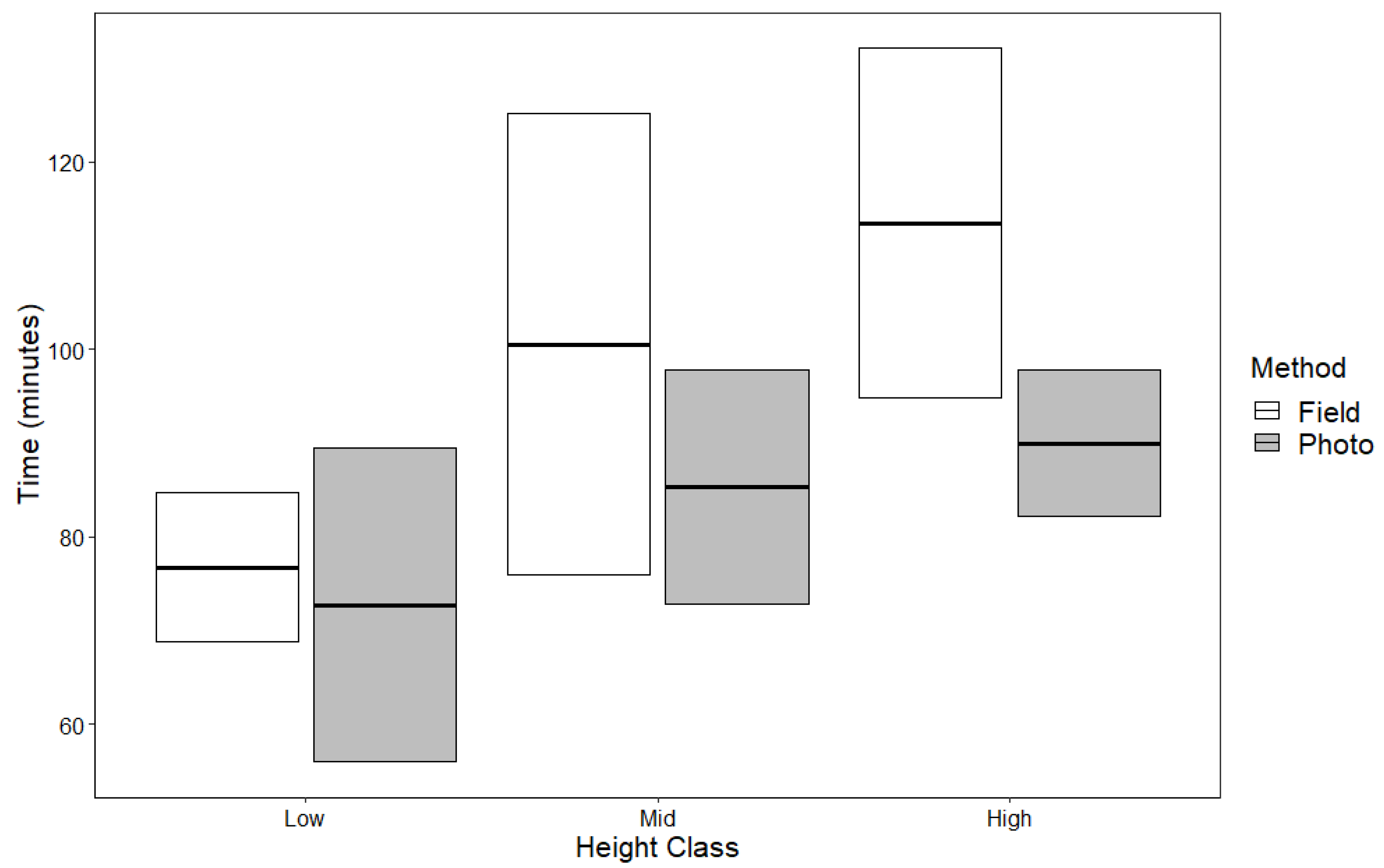
The image-based method was overall more efficient than the point-intercept surveys, reducing total survey time by an average of 13 to 46 min per plot depending on the configuration (Table 1; paired sample t-test, p = 0.09 for configuration 1). When comparing the time efficiency of the two methods within different types of vegetation, we found that the image-based method had higher efficiency in taller vegetation than in low vegetation. There was a mean increase of 23.9 min to complete a field survey versus image-based survey in the tallest vegetation height class, whereas the increase was only 6.6 min within the lowest vegetation height plots (Figure 6). Results of a linear mixed effects model with time as the response variable showed no significant effects of method (F1,10 = 2.8, p > 0.10), height class (F2,10 = 2.09, p > 0.10), or their interaction (F2,10 = 0.40, p > 0.10); however, there was a trend showing reduced survey time with the image-based method in taller vegetation (Figure 6).

Figure 6.
Survey time in minutes by survey method and vegetation height class. Height classes were low (<1 m), mid (1 m to 1.5 m), and high (>1.5 m). Crossbars represent the mean ±95% confidence interval for 13 field plots within three vegetation height classes surveyed in 2019 by both the point-intercept and Photogrid methods. There were no significant effects of method, height class, or their interaction on survey time. The graph is provided to illustrate a trend that the photo method time was lower in mid and high height classes.
4. Discussion
With the increasing prominence of using remote-sensing imagery to estimate metrics of plant diversity [7,8,9,10,11,12], there is a concomitant need to develop new methods to rapidly measure diversity on the ground. Our method is an alternative to ground surveys that efficiently sampled vegetation in large plots over rugged terrain. Such methods will be needed to collect a sufficient number of calibration and validation points for forthcoming global imaging-spectroscopy missions such as NASA’s SBG [16], which have specified mission objectives for characterizing metrics related to diversity.
When compared to a traditional point-intercept field sampling method, the image-based method provided comparable results for measures of Simpson’s species diversity (1/D) and percent cover of individual cover classes, while reducing time and effort to collect these data in the field. There was high correlation between point-intercept and image-based survey results and the Photogrid sampling effort (configuration) did not lead to significantly different estimates of percent cover. By using the lowest sampling effort (configuration 12) the amount of time to complete a Photogrid survey could be reduced by up to 46 min per plot without compromising the accuracy of the percent-cover estimates. This made the image-based method substantially more efficient than a traditional ground survey for estimating percent cover.
When investigating the differences in percent-cover estimates among cover classes, we found the image-based method to have the greatest accuracy for the most abundant classes (Supplementary Materials S1: Figure S2, Table S6). In addition, the image-based method produced lower values for percent cover for species that were small-statured (eg. Cryptantha sp., a small white-flowering herb) or sparse in their cover (Acmispon glaber, dead shrub), which is likely due to the difficulty in observing these classes in the photos compared to in-person in the field. These classes are important for the overall biodiversity of the community, but have less influence on the total vegetative cover due to their lower abundances. Therefore, the performance of the image-based method in classifying abundant species makes it useful for map calibration and validation but may limit it for other more diversity-focused applications.
Furthermore, the results for species richness (S) and evenness (E) were mixed when traditional point-intercept surveys were replaced by image-based surveys. Species-richness estimates were generally higher in the field, systematically so by an average of 3.6 species across all types of plots in 2018, but only by less than one species in 2019 (Figure 4 and Figure 5c; Supplementary Materials S1: Table S1). Surveyors were able to more easily see small and less abundant species in the field that were more difficult to identify in the photos or were missed altogether through the generation of gridpoints by the Photogrid program. As well, many smaller-statured species are likely obscured by the overstory, an observation that is likely to make image-based methods untenable for total richness in forested plots, although in many ecosystems remote sensing is only sensitive to overstory richness in forests. A few species could only be identified to a genus or functional group using photos (e.g., annual grasses), whereas they could be identified to species in the field. This was uncommon and mostly occurred with non-native annual grasses, which could lead to recording one or two species more in field surveys. In addition, as the photo-sampling effort decreased, the difference between point-intercept and image-based results for species richness and evenness became larger with increasingly less accuracy for the image-based method (Supplementary Materials S1: Table S1; Figure 5).
While our larger field effort took place during the first year of the study when species percent cover was estimated within 83 plots, we did not conduct quantitative field sampling of each plot using a traditional field-based method. However, we did perform an exhaustive visual survey to identify the number of species present, and the difference in richness followed the same trend found in the survey conducted in 2019, i.e., that field sampling recorded more species present. In 2018, it is notable that image-based estimates of richness were closer to field estimates of richness for the steeper plots than the flat plots. This result may occur because transects for steep plots were laid at the top of the slope along a flat trail or road, with images collected downslope of the flat area that could be traversed safely, whereas transects for flat plots were laid across the sampled area, and the field crew could traverse the entire sampling area. This difference in the ability to traverse the plots may account for species being missed in the field in steep areas. This finding highlights the general issue that the steep and dangerous terrain within the majority of this region make it impossible to use traditional field survey methods to “ground-truth” the image-based data for these plots.
As such, 16 new plots were chosen during the second-year validation study with more moderate, traversable slopes well-suited for more high-effort field surveys in addition to the image-based surveys. The results of our validation experiment confirmed the effectiveness and accuracy of the image-based method; however, our validation was limited to only the Flat Protocol due to safety concerns with traversing steep plots. Based on our experience using these protocols in a variety of settings, we think the Steep Protocol is more accurate than visual estimation for collecting percent-cover data; however, we lack a quantitative assessment of this accuracy. The fact that our small-scale and highly controlled study faced such impediments in accessing reliable ground-truthing data suggests this is likely a universal problem in remote-sensing and other ecological studies involving steep or otherwise hazardous terrain. This limitation highlights the importance of this tool in problematic landscapes that are typical of MTEs, which feature both steep terrain and a heterogeneous composition of short- and mid-statured vegetation.
The sampling method with a camera on a pole seems best utilized in ecosystems such as MTEs, which are dominated by shrubs or large bunch grasses that can be identified easily with semi-aerial images. Species identification from photos could be difficult in ecosystems with many small-statured species, such as some grasslands, but could still be used in these ecosystems to map broader cover classes such as photosynthetic and non-photosynthetic vegetation [24,34]. It is also worth reiterating that in some settings, an image-based method may be the only safe and efficient approach to collect a sufficient sample size of data. We used a camera affixed to a telescoping fiberglass pole, but the image-sampling method could also be applied to data from an unmanned aerial system (UAS) or airborne imagery. Certainly, image acquisition from a drone would be necessary for the method to be used in tall vegetation such as forests or in very steep canyons, but as noted previously, the method would miss large numbers of understory species in such environments. More generally, though, the operation of UASs for data collection in remote environments may be difficult. For species identification of low-stature vegetation such as in our study and characteristic of MTEs, a UAS may need to be flown at a low altitude in which air movement by propellers may preclude the identification of species. This can be mitigated by higher flight altitudes using higher-resolution cameras. However, there can also be logistical issues with UASs, including transport into remote sites, restrictions related to line-of-site flying, and safety concerns when flying at low altitudes in steep terrain. Although low-tech, the extendable pole was easily transported into the field and deployed by a team of three to rapidly collect imagery over the shrubland vegetation at our sites. In some conditions, using a camera on a pole will be more affordable and logistically simpler than surveys with an UAS.
5. Conclusions
The implications of these results vary depending on the application of the survey method. To meet certain biodiversity assessment goals highly influenced by species richness, the image-based method will fall short in its failure to identify all species, especially those occurring in the understory. A more appropriate application for the method is in broader-scale habitat mapping, and to capture spatial or temporal trends in diversity metrics rather than the correct absolute values of those metrics, such as global comparisons of biodiversity trends across MTEs. As well, this method should work well to capture the total cover and abundance of common or physiognomically large species, and it had its greatest efficiency in sampling vegetation more than 1 m tall (Figure 6). The spatial scale and image resolution of our surveys were appropriate for identifying the required species and composition patterns of many described plant communities and vegetation alliances commonly found in MTEs. This resolution was also ideally suited to calibrating vegetation maps derived from imaging spectroscopy for southern California shrublands (Bonfield et al., manuscript in preparation). An added value of this method is the ability to store the images for archival purposes or for future analysis for a different purpose [23,24,27].
Ultimately, the metric most important for validation of imaging spectroscopy is the percent cover of each species, which was found to be reliably measured on the plot scale by the image-based method (Figure 5B) and for dominant individual species (Supplementary Materials S1: Figure S2). Image-based surveys require less effort to perform compared to more traditional field surveys, and they also open up some areas to ground-truthing that may have gone previously un-surveyed due to hazardous or steep terrain. As remote sensing of vegetation continues to be a common and relied-upon technique for collecting ecological data, it is increasingly important for ground-truthing efforts to match the levels of quality necessary to confidently assess the calibration and validity of these efforts, and at an equal pace to the evolving technology. This image-based sampling method can be used in a variety of applications for these purposes.
Supplementary Materials
The following supporting information can be downloaded at: https://www.mdpi.com/article/10.3390/rs14081933/s1, Figure S1: Distribution of elevation (m) and slope (degrees) values within plots and entire fire scar perimeters for the Copper fire and Sayre fire within the Angeles National Forest; Table S1: Mean and standard deviation of diversity metrics for the 12 configurations of Photogrid sampling and the field point-intercept method; Table S2: Results of linear models with % Coverp-i as the response variable and % Coverp as the predictor variable, Table S3: Results of linear models with 1/Dp-i as the response variable and 1/Dp as the predictor variable; Table S4: Results of linear models with Sp-i as the response variable and Sp as the predictor variable; Table S5: Results of linear models with Ep-i as the response variable and Ep as the predictor variable; Figure S2: Linear regressions between % Coverp and % Coverp-i for 10 species occurring in 9 or more of the 16 plots surveyed in 2019; Table S6: Linear model results for % Coverp predicted by % Coverp-i for 10 species and ground cover classes occurring in 9 or more of the 16 plots surveyed in 2019.
Author Contributions
Conceptualization, S.B., D.S., E.N.S., P.A.T., M.A. and E.J.Q.; methodology, N.L., E.N.S., P.A.T., M.A. and E.J.Q.; investigation, E.N.S., P.A.T., M.A. and E.J.Q.; data curation M.A. and E.J.Q.; writing—original draft preparation, M.A. and E.J.Q.; writing—review and editing, M.A., N.L., E.N.S., P.A.T., S.B., D.S. and E.J.Q.; funding acquisition, S.B., D.S. and E.J.Q. All authors have read and agreed to the published version of the manuscript.
Funding
This project was funded by the National Fish and Wildlife Foundation, a NASA HBCU/MI award, and the California State University Agricultural Research Institute (19-04-108).
Open Research Statement
The Photogrid code is publicly shared on GitHub (Liu, Singh and Townsend, https://github.com/EnSpec/PhotoGrid).
Data Availability Statement
The data presented in this study are available on request from the corresponding author. The data are not publicly available due to data concerning sensitive species.
Acknowledgments
We thank T. Edwards, S. Estrada, R. Fitch, G. Hernandez, S. Laumann, J. Martinez, M. Martinez, M. Mazhnyy, A. Ongjoco, and L. Tucker for assistance with data collection. Thank you to A. Berger for programming assistance and A. Singh for creating the first versions of Photogrid.
Conflicts of Interest
The authors declare no conflict of interest.
References
- Myers, N.; Mittermeier, R.A.; Mittermeier, C.G.; da Fonseca, G.A.; Kent, J. Biodiversity hotspots for conservation priorities. Nature 2000, 403, 853–858. [Google Scholar] [CrossRef] [PubMed]
- Cowling, R.M.; Rundel, P.W.; Lamont, B.B.; Arroyo, M.K.; Arianoutsou, M. Plant diversity in mediterranean-climate regions. Trends Ecol. Evol. 1996, 11, 362–366. [Google Scholar] [CrossRef]
- Rundel, P.W.; Arroyo, M.T.K.; Cowling, R.M.; Keeley, J.E.; Lamont, B.B.; Pausas, J.G.; Vargas, P. Fire and plant diversification in mediterranean-climate regions. Front. Plant Sci. 2018, 9, 851. [Google Scholar] [CrossRef] [PubMed]
- Rundel, P.W.; Arroyo, M.T.K.; Cowling, R.M.; Keeley, J.E.; Lamont, B.B.; Vargas, P. Mediterranean biomes: Evolution of their vegetation, floras, and climate. Annu. Rev. Ecol. Syst. 2016, 47, 383–407. [Google Scholar] [CrossRef]
- Underwood, E.C.; Franklin, J.; Molinari, N.A.; Safford, H.D. Global change and the vulnerability of chaparral ecosystems. Bull. Ecol. Soc. Am. 2018, 99, e01460. [Google Scholar] [CrossRef] [Green Version]
- Cox, R.L.; Underwood, E.C. The importance of conserving biodiversity outside of protected areas in mediterranean ecosystems. PLoS ONE 2011, 6, e14508. [Google Scholar] [CrossRef]
- Rocchini, D.; Boyd, D.S.; Féret, J.B.; Foody, G.M.; He, K.S.; Lausch, A.; Nagendra, H.; Wegmann, M.; Pettorelli, N. Satellite remote sensing to monitor species diversity: Potential and pitfalls. Remote Sens. Ecol. Cons. 2016, 2, 25–36. [Google Scholar] [CrossRef]
- Colgan, M.S.; Baldeck, C.A.; Feret, J.B.; Asner, G.P. Mapping Savanna Tree Species at Ecosystem Scales Using Support Vector Machine Classification and BRDF Correction on Airborne Hyperspectral and LiDAR Data. Remote Sens. 2012, 4, 3462–3480. [Google Scholar] [CrossRef] [Green Version]
- Féret, J.B.; Asner, G.P. Mapping tropical forest canopy diversity using high-fidelity imaging spectroscopy. Ecol. Appl. 2014, 24, 1289–1296. [Google Scholar] [CrossRef]
- Hochberg, E.J.; Roberts, D.A.; Dennison, P.E.; Hulley, G.C. Special issue on the Hyperspectral Infrared Imager (HyspIRI): Emerging science in terrestrial and aquatic ecology, radiation balance and hazards. Remote Sens. Environ. 2015, 167, 1–5. [Google Scholar] [CrossRef]
- Singh, A.; Serbin, S.P.; McNeil, B.E.; Kingdon, C.C.; Townsend, P.A. Imaging spectroscopy algorithms for mapping canopy foliar chemical and morphological traits and their uncertainties. Ecol. Appl. 2015, 25, 2180–2197. [Google Scholar] [CrossRef] [PubMed] [Green Version]
- Wang, R.; Gamon, J.A. Remote sensing of terrestrial plant biodiversity. Remote Sens. Environ. 2019, 231, 111218. [Google Scholar] [CrossRef]
- Asner, G.P.; Martin, R.E. Spectranomics: Emerging science and conservation opportunities at the interface of biodiversity and remote sensing. Glob. Ecol. Conserv. 2016, 8, 212–219. [Google Scholar] [CrossRef] [Green Version]
- Seeley, M.; Asner, G.P. Imaging Spectroscopy for Conservation Applications. Remote Sens. 2021, 13, 292. [Google Scholar] [CrossRef]
- Cavender-Bares, J.; Gamon, J.A.; Townsend, P.A. The Use of Remote Sensing to Enhance Biodiversity Monitoring and Detection: A Critical Challenge for the Twenty-First Century. In Remote Sensing of Plant Biodiverstiy; Cavender-Bares, J., Gamon, J.A., Townsend, P.A., Eds.; Springer: Cham, Switzerland, 2020. [Google Scholar] [CrossRef]
- National Academies of Sciences, Engineering, and Medicine. Thriving on Our Changing Planet: A Decadal Strategy for Earth Observation from Space; The National Academies Press: Washington, DC, USA, 2018. [Google Scholar]
- Schimel, D.S.; Townsend, P.A.; Pavlick, R. Prospects and Pitfalls for Spectroscopic Remote Sensing of Biodiversity at the Global Scale. In Remote Sensing of Plant Biodiverstiy; Cavender-Bares, J., Gamon, J.A., Townsend, P.A., Eds.; Springer: Cham, Switzerland, 2020. [Google Scholar] [CrossRef]
- Washington-Allen, R.A.; West, N.E.; Ramsey, R.D.; Efroymson, R.A. A Protocol for Retrospective Remote Sensing-Based Ecological Monitoring of Rangelands. Rangel. Ecol. Manag. 2006, 59, 19–29. [Google Scholar] [CrossRef]
- West, N.E. Theoretical underpinnings of rangeland monitoring. Arid Land Res. Manag. 2003, 17, 333–346. [Google Scholar] [CrossRef]
- West, N.E. History of rangeland monitoring in the USA. Arid Land Res. Manag. 2003, 17, 495–545. [Google Scholar] [CrossRef]
- Washington-Allen, R.A. Retrospective Ecological Risk Assessment Commercially-Grazed Rangelands Using Multitemporal Satellite Imagery. Ph.D. Thesis, Utah State University, Logan, UT, USA, 2003. [Google Scholar]
- Booth, T.D.; Cox, S.E.; Fifield, C.; Phillips, M.; Williamson, N. Image Analysis Compared with Other Methods for Measuring Ground Cover. Arid Land Res. Manag. 2005, 19, 91–100. [Google Scholar] [CrossRef]
- Booth, D.T.; Cox, S.E. Art to science: Tools for greater objectivity in resource monitoring. Rangelands 2010, 33, 27–34. [Google Scholar] [CrossRef] [Green Version]
- Booth, D.T.; Cox, S.E. Image-based monitroing to measure ecological change in rangeland. Front. Ecol. Environ. 2008, 6, 185–190. [Google Scholar] [CrossRef] [Green Version]
- Moffet, C.A.; Taylor, J.B.; Booth, D.T. Postfire Shrub Cover Dynamics: A 70-Year Fire Chronosequence in Mountain Big Sagebrush Communities. J. Arid. Environ. 2015, 114, 116–123. [Google Scholar] [CrossRef] [Green Version]
- Cagney, J.; Cox, S.E.; Booth, D.T. Comparison of Point Intercept and Image Analysis for Monitoring Rangeland Transects. Rangel. Ecol. Manag. 2011, 64, 309–315. [Google Scholar] [CrossRef]
- Booth, D.T.; Cox, S.E.; Berryman, R.D. Point sampling digital imagery with ‘Samplepoint’. Environ. Monit. Assess. 2006, 123, 97–108. [Google Scholar] [CrossRef] [PubMed]
- Cotillon, S.; Mathis, M. Tree Cover Mapping Tool—Documentation and User Manual; U.S. Geological Survey: Reston, VA, USA, 2016; 11p.
- LARIAC. 3-Foot Digital Elevation Model (DEM). 2016. Available online: https://lariac-lacounty.hub.arcgis.com (accessed on 8 April 2022).
- Sony Electronics Inc. PlayMemories Mobile; [Imaging Edge Mobile], 6.2.0; Sony Electronics Inc.: San Diego, CA, USA; Available online: https://imagingedge.sony.net/en-us/ie-mobile.html (accessed on 8 April 2022).
- Lenth, R.V. emmeans: Estimated Marginal Means, aka Least-Squares Means; U.S. Geological Survey: Reston, VA, USA, 2021.
- R Core Team. R: A language and Environment for Statistical Computing, R Foundation for Statistical Computing: Vienna, Austria. 2020. Available online: http://www.r-project.org/index.html (accessed on 8 April 2022).
- Bates, D.; Machler, M.; Bolker, B.M.; Walker, S.C. Fitting linear mixed-effects models using lme4. J. Stat. Softw. 2015, 67, 1–48. [Google Scholar] [CrossRef]
- Roberts, D.A.; Smith, M.O.O.; Adams, J.B.B. Green vegetation, nonphotosynthetic vegetation, and soils in AVIRIS data. Remote Sens. Environ. 1993, 44, 255–269. [Google Scholar] [CrossRef]

Publisher’s Note: MDPI stays neutral with regard to jurisdictional claims in published maps and institutional affiliations. |
© 2022 by the authors. Licensee MDPI, Basel, Switzerland. This article is an open access article distributed under the terms and conditions of the Creative Commons Attribution (CC BY) license (https://creativecommons.org/licenses/by/4.0/).