Abstract
An approach to developing a blended satellite-rainfall dataset over Australia that could be suitable for operational use is presented. In this study, Global Satellite Mapping of Precipitation (GSMaP) satellite precipitation estimates were blended with station-based rain gauge data over Australia, using operational station data that has not been harnessed by other blended products. A two-step method was utilized. First, GSMaP satellite precipitation estimates were adjusted using rain gauge data through multiplicative ratios that were gridded using ordinary kriging. This step resulted in reducing dry biases, especially over topography. The adjusted GSMaP data was then blended with the Australian Gridded Climate Dataset (AGCD) rainfall analysis, an operational station-based gridded rain gauge dataset, using an inverse error variance weighting method to further remove biases. A validation that was performed using a 20-year range (2001 to 2020) showed the proposed approach was successful; the resulting blended dataset displayed superior performance compared to other non-gauge-based datasets with respect to stations as well as displaying more realistic patterns of rainfall than the AGCD in areas with no rain gauges. The average mean absolute error (MAE) against station data was reduced from 0.89 to 0.31. The greatest bias reductions were obtained for extreme precipitation totals and over mountainous regions, provided sufficient rain gauge availability. The newly produced dataset supported the identification of a general positive bias in the AGCD over the north-west interior of Australia.
1. Introduction
Precipitation is vital for life on earth and is a fundamental part of Earth’s water cycle and climate system [1]. Measuring variations in its intensity, duration and frequency are vital to enabling efficient water management and water-related disaster responses.
The traditional method of measuring rainfall involves in-situ rain gauges. These provide a direct measurement of surface rainfall but also possess certain limitations. Being point-based measurements, rain gauges may not be able to provide an accurate spatial representation of rainfall over an area. Gridded rainfall analyses can be generated from point-based station data by applying objective analysis methods, but their accuracy is hindered in poorly observed areas [2,3]. This is a concern, as rain gauge installation can be economically or physically unfeasible over large parts of the world, including over oceans [4].
In areas where rain gauge density is low, the ability to accurately assess rainfall is impacted, especially as rainfall is a variable that can exhibit a high degree of spatial variation [3]. Furthermore, rain gauge estimates are also subject to instrumental errors [5] as well as sampling biases [6,7,8].
Satellites provide an efficient method for uniformly assessing rainfall over a quasi-global domain [9]. Modern methods use microwave sensors to detect the emission and scattering of radiation from hydrometeors and link these to rain rates through forward model calculations [10]. Contemporary satellite products have exhibited good performance, rivalling or outperforming climate reanalyses under certain conditions [11]. However, significant biases still exist due to the nature of the sampling process and the algorithms used [12].
By blending in station rain gauge data, these biases can be reduced, especially where station density is high. The blending of station data with satellite precipitation estimates has been attempted previously using a variety of techniques. These include the use of ordinary kriging [13], Bayesian kriging [14], co-kriging [15] and conditional merging by kriging [16], and in most cases such techniques has been effective in improving accuracy [14,15,16,17]. However, the majority of these studies have been completed for other regions, with few being specific to Australia.
Focusing specifically on Australia, [18] attempted to blend TRMM-3B42RT satellite and rain gauge data using a variety of kriging methods and found the value of blending was generally difficult to discern. However, there was improvement where the gauge density was approximately less than 4 gauges per 10,000 km2, and the uncertainty of the analysis decreased with the inclusion of satellite data. On a much smaller scale, [17] evaluated blending techniques based on kriging, inverse-distance weighting and a radial basis function over two Australian river catchments. The kriging-based methods performed the best, and the use of elevation as an additional variable through co-kriging was valuable.
Currently, the only blended satellite rainfall dataset provided by the World Meteorological Organization’s (WMO) Space-based Weather and Climate Extremes Monitoring (SWCEM) is the blended version of Climate Prediction Center Morphing technique dataset (CMORPH-BLD), which uses the CMORPH satellite dataset as a first guess and then blends in observations from the CPC Unified Gauge-Based Analysis of Global Daily Precipitation (CPC Unified) dataset through optimal interpolation [19]. An improvement from this technique was identified for Australia but not for Papua New Guinea (PNG), where CMORPH-BLD was actually slightly inferior to GSMaP, an unblended dataset [20]. A likely reason for this disparity is the lack of stations over PNG in the CPC Unified dataset, especially compared to over Australia, a difference likely in the order of two magnitudes or more [19].
This motivated us to undertake a study to investigate if the SWCEM datasets can be improved if a denser rain gauge network is used for blending. The Bureau of Meteorology (BOM) Australian Data Archive for Meteorology (ADAM) contains over 6700 Bureau-maintained stations that meet the International Civil Aviation Organization (ICAO) standards, with the CPC Unified dataset only including a subset of these stations. The main objective of this study was to explore the blending of SWCEM datasets using a fuller set of station data over Australia, with a focus on operational usage. An important aspect of the technique in this study is that it will be developed to be modular and open-source, meaning it can be used with any set of satellite and station data, and thereby by users globally. The blended product, along with validation will be conducted on a monthly timescale, reflecting its intended use for climatological applications such as drought monitoring. An in-depth validation on the newly produced dataset is needed to determine whether the procedure has value.
Although the blending method developed draws from existing techniques, the novelty of this study lies in its focus over Australia, along with its use of operational station data that has not been harnessed by other blended products. The significance of these points is described below:
- The utilization of operational station data, along with the use of the Australian Gridded Climate Data (AGCD) rainfall analysis, has great potential to create improved satellite-based rainfall datasets for operational use in Australia. This would be particularly useful for poorly observed areas such as over the interior of the nation, where further improvements in accuracy would require uneconomical investments in expanding the rain gauge network [3]. Existing blended datasets have not made full use of this operational data.
- As the first blended dataset to take advantage of the full set of operational station data available in Australia, its increased accuracy over stations will allow AGCD to be better validated, providing original insights into its weaknesses over gauge-sparse regions. This knowledge is important for future advancements in AGCD.
- A focus on the Australian domain allows for a more complete and thorough analysis of the blending technique, including the identification of spatial performance patterns specific to the region. Few studies have focused on Australia, and those which have did not use the full operational set of data or were not completed on a nation-wide basis.
2. Materials and Methods
2.1. Study Area
Figure 1 shows a map of the domain used in this research along with a depiction of its topography and coverage by BOM rain gauges. The continental landmass is relatively flat with the main orographic feature being the Great Dividing Range (GDR), a mountain range that runs from the north-eastern tip of Queensland, along the east coast of Australia and into central Victoria.
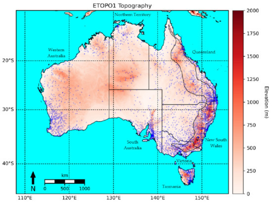
Figure 1.
Map of study area showing ETOPO1 elevation as well as typical rain gauge coverage. Location of the rain gauge stations are depicted as blue dots. Note the significant topography along the east coast of Australia; this is the GDR with the light gray outline depicting its approximate extent.
The number of rain gauges available for reporting varies from month to month due to factors such as changes in historical availability (e.g., from installation and decommissioning) and data quality control. The stations from December 2020 were depicted as this month contained the fewest number of reporting stations (4346) across the study period.
Of particular significance are the very low rain gauge densities over central parts of the country. The topography is derived from NOAA’s ETOPO1 bedrock dataset, a 1-arc minute global relief model that provides information on land topography and ocean bathymetry [21].
Australia possesses a range of climate zones [22]. Northern parts of the country experience a tropical climate where most of the rainfall is driven by the monsoon during the wet season (October to April), with little rainfall occurring during the other months of the year [23]. Large parts of the interior are considered arid, generally observing very little rainfall. Proximity to moisture sources is low, with the main source of rainfall being north-west cloud bands, which leads to rainfall being highly variable and temporally concentrated [23]. Temperate regions exist to the south-east and south-west, where the majority of the rainfall occurs during the southern wet season (April to November) and is associated with frontal systems [23]. Increased proximity to the coast and elevation tend to be positively correlated to rainfall. The greatest rainfall amounts are usually observed over western Tasmania (largely produced by frontal systems and enhanced by orography) and the northern tropical coasts (associated with tropical convective modes over the wet season).
2.2. Datasets
The satellite dataset used for developing the adjusted and blended products in this study is GSMaP Gauge-Adjusted Near Real Time, hereafter referred to as GSMaP, which is produced by the Japan Aerospace Exploration Agency (JAXA) [24]. The version used is Version 6, as this is the version available to the SWCEM program. In our earlier studies, we demonstrated the better performance of GSMaP compared to CMORPH-CRT in both Australia and PNG [20,25]. AGCD and MSWEP are used in the correction and blending techniques. Additionally, two other satellite-based datasets (GSMaP-gauge and CMORPH-BLD) and a non-satellite-based dataset (ERA5) are included for validation. Details on the datasets used in this study are presented in Table 1.

Table 1.
Details on datasets used in this study. The datasets used as inputs for the final blended product are shaded.
An understanding of the biases of these datasets is pertinent for understanding the results generated in this study. Previous studies have identified systematic biases that exist in satellite estimates [31,32]. Their performance can be severely reduced over orography, with the underestimation of rainfall occurring at higher elevations [33,34]. This underestimation is compounded by the poor detection of snowfall and contamination from cold surfaces, particularly during winter [35]. Underestimation is also common for very low and very high rainfall rates [36,37]. The former is due to the signal from these rates being weak as well as a prevalent mode for these rainfall rates being from warm low clouds which are more difficult for satellites to detect [9]. The latter can be related to how the development of convective rainfall may not be well-captured between satellite passes [9]. Satellite retrieval algorithms can also encounter difficulties around large waterbodies due to confusion about the surface types, leading to overestimation in terms of the precipitation amount and frequency [38,39,40].
Additionally, gridded datasets smooth the data, resulting in the overestimation (underestimation) of very low (high) totals when compared to point-based totals [41]. This point is also relevant to the non-satellite-based datasets.
Reanalysis data has been documented to underestimate high totals and overestimate the frequency and volume of low totals [42,43]. Over complex terrain in Turkey, [44] found contemporary satellite products had an overall wet bias but for wet regions, a dry bias was observed. ERA5 displayed a consistent wet bias, and all products reduced in performance as the slope of the region increased [44].
The greatest control on accuracy for gauge-based datasets such as AGCD is the density of the underlying rain gauge network [45]. AGCD can be expected to have its greatest biases over the gauge sparse parts of Australia’s interior. MSWEP is another dataset used in this study. Since it is formed from satellite, gauge and reanalysis data, it will inherit the biases from its input data as well as possess an additional uncertainty imposed by the blending process. In a global comparison to a variety of contemporary rainfall datasets, MSWEP V2 was found to demonstrate the highest skill, being able to take advantage of the respective strengths of each data source [43].
2.3. Adjusted and Blended GSMaP Development Methods
The method used to develop a monthly GSMaP-AGCD blended product was inspired by earlier studies that employed a two-step process [16,19,46]. The steps involved are outlined:
- Reducing systematic bias and random errors in the satellite dataset through an adjustment based on ADAM gauge data. For this product, this bias correction was performed by attempting to match the GSMaP dataset more closely to the rain gauge data using corrective multiplicative ratios. A similar method of bias correction was performed by [16,46,47,48], with [48] finding it to be the most performant scheme, outperforming elevation zone correction, a power transform based correction, distribution transformation and empirical quantile mapping. Linear correction via kriging was also used by [13] over Pakistan, outperforming other schemes based on inverse-distance weighting, polynomial interpolations and radial basis functions. Over a river catchment in Australia, [49] compared linear correction using ordinary kriging against inverse-distance weighting and kriging with genetic programming, and found that ordinary kriging performed the best.
- The value of the satellite dataset at the location of each rain gauge was obtained by bilinearly interpolating the gridded values to the coordinates of the station. Note that the interpolation of a gridded value to a point still refers to an areal average, just centered upon that point.
- A set of multiplicative ratios was then calculated by dividing the station values by the interpolated satellite values. The set of ratios was then clipped to be between 0.1 and 10, limiting the adjustment to an order of magnitude. A total of 74,711 out of 1,400,754 values were clipped, or around 5.3%.
- This set was then converted into a grid using ordinary kriging. Kriging is an interpolation method that estimates an unknown value based on the statistical relationship of known points in a local neighborhood [50]. Ordinary kriging is the most widely used form and assumes a constant mean and variogram across the whole domain [50]. The unknown value is a weighted average of known values, with the weights being determined from a set of equations constrained by minimizing the estimation variance, in conjunction with the condition that the weights must sum to one [50]. The Python module PyKrige was used, with multiple variogram models tested—linear, power, Gaussian, spherical and exponential—with the exponential model being chosen as it demonstrated the best performance (see Appendix A). A resolution of 0.25° was used instead of the native 0.1° of GSMaP due to computing memory restrictions on our research environment. A higher resolution variant could be produced for operational usage though preliminary validation did not show much improvement when testing the finer resolution (the metrics scores improved by less than 2%). The pseudo-inverse matrix was solved to improve stability. It was computed using the singular value decomposition method, which was faster than via the least-squares solution. The result of kriging was a grid of multiplicative ratios to apply to the GSMaP dataset to form the adjusted GSMaP dataset, hereafter known as GSMaP-adj.
- Blending GSMaP-adj with AGCD, with the intention of more heavily utilizing GSMaP-adj when and where it was superior to the gauge-based analysis. To achieve this, inverse-variance weighting was employed.
- GSMaP-adj was bilinearly interpolated to 0.1° to match AGCD. The error variances from both GSMaP-adj and AGCD (using MSWEP as truth) were calculated across the entire domain for each month. This allowed both spatial and seasonal variations to be accounted for. The difference between the variances of the two datasets is shown in Appendix B. Even though MSWEP has its own biases, its inclusion of gauge, satellite and reanalysis data, along with its homogeneity over space, is valuable as a reference dataset for inverse-variance weighting, with the process combining the accuracies of GSMaP-adj and AGCD with the spatial pattern of MSWEP.
- The merged product, hereafter known as GSMaP-bld, is then a weighted average of GSMaP-adj and AGCD, with the weights being determined by the size of the error variances with respect to each other. The larger the error variance, the lesser the weight that dataset has on the weighted average. It is represented in Equation (1):where σ2 is the error variance, x is the value at a grid cell and the subscripts GB, GA and A refer to the datasets GSMaP-bld, GSMaP-adj and AGCD, respectively.
A visualization of the entire process is shown in Figure 2.
Figure 2.
Processes involved in developing the adjusted and blended versions of GSMaP.
2.4. Validation Method
Both point-based and gridded validation were performed on a monthly basis from 2001 to 2020 across the Australian domain. For the point-based validation, all the datasets were compared to rain gauge values from the ADAM database. To obtain a value from a gridded dataset that corresponded to a point, the data from the gridded dataset were bilinearly interpolated to a point that corresponded to the location of a rain gauge. All the datasets introduced in Section 2.2 (GSMaP, GSMaP-adj, GSMaP-bld, AGCD, ERA5, MSWEP and CMORPH-BLD) were validated. Additionally, a blended GSMaP that used the raw GSMaP rather than the adjusted GSMaP (hereafter termed GSMaP-raw-bld) was also evaluated to determine if the adjustment process was a valuable step.
Following the results of the point validation, GSMaP, GSMaP-adj, GSMaP-bld, ERA5 and MSWEP were compared to AGCD for the gridded validation. The gridded validation was performed over the Australian domain, specifically over the longitudes of 108°E to 156°E and the latitudes of 45°S to 9°S, with a land-only mask applied. These datasets were bilinearly interpolated to a resolution of 0.1°. This was the most common native resolution across the datasets. Only land values across the domain were compared with the Python module Basemap used to mask the data over the ocean.
The validation metrics used to assess bias were the mean bias (MB), mean absolute error (MAE) and the root-mean-squared-error (RMSE). The MAE is less sensitive than the RMSE to outliers. The MAE was also divided by the mean rainfall to obtain the normalized mean absolute error (Norm. MAE), which removed the effect of larger rainfall values leading to larger errors. To assess correlation, the Pearson correlation coefficient (R) was used. To assess the similarity in spread across the datasets, the differences in the standard deviation, the mean and the coefficient of variation (CV), which is the ratio of the standard deviation to the mean of the dataset, were analyzed. The equations for the metrics are summarized in Table 2, with Ei representing the estimated value at a point or grid box i, Oi being the value taken as truth and N being the number of samples (the number of stations or grid cells).
Table 2.
Summary of equations for the metrics used.
Additionally, hit rates on the success of the datasets reproducing the top and bottom quintiles of the truth dataset were also calculated to assess their performance in capturing extremes. The percentile rank of each grid point in AGCD was computed for all the months. If that data point was within the top (bottom) quintile, the percentile rank of the corresponding point in the other datasets was compared with a hit being registered if its percentile rank was also in the top (bottom) quintile.
All the datasets used in this study contain a degree of station influence (apart from ERA5). Ideally, a form of split-sample validation should have been performed to remove the inflation of skill due to the repeat of stations in both the datasets being validated and the validation set itself. This would have resulted in an inflated representation of out-of-sample accuracy. However, as some of the comparison datasets were generated by different organizations, there was no way to regenerate these datasets using just a subset of the stations, and split-sample validation could not be performed. Finding a reference dataset which has a reasonable level of accuracy but which also does not contain station influence is difficult and will be addressed in a future study.
These metrics were calculated monthly for all land grid cells or station points in the domain. A bulk average for these metrics was then calculated by averaging over the validation period. When the results were categorized by seasons, the austral seasons of summer (December, January and February, or DJF), autumn (March, April and May, or MAM), winter (June, July and August, or JJA) and spring (September, October and November, or SON) were used.
3. Results
3.1. Point Validation
The results of the general comparison of satellite precipitation estimates to station rain gauge data are shown in Figure 3.
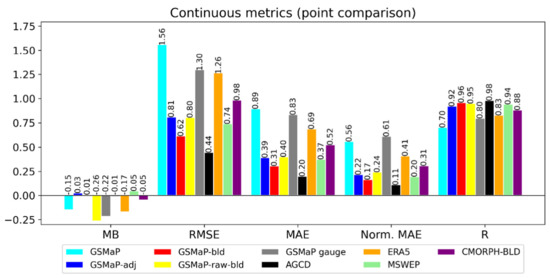
Figure 3.
Validation metrics using gauge data at point locations as truth. Mean bias (MB), root-mean-squared-error (RMSE), mean absolute error (MAE), normalized mean absolute error (Norm. MAE) and Pearson’s correlation coefficient (R) are shown. The units of MB, RMSE and MAE are in mm/day, while Norm. MAE and R are unitless. A perfect score for each metric would be 0, except for R where 1 is perfect.
The adjustment and blending process appears to have improved the accuracy of GSMaP. For example, the normalized MAE of GSMaP-adj (0.22) was less than half of the raw version (0.56), with GSMaP-bld exhibiting an even further reduction (0.17). Both the adjusted and blended versions were better than ERA5 (0.41). Such substantial improvements can be expected, as the stations used for adjustment were also those used in the validation.
Using unadjusted GSMaP in the blending process (GSMaP-raw-bld) yielded a significantly worse performance across all the bias metrics than when adjusted GSMaP was used. For example, the RMSE increased by around 33% when unadjusted GSMaP was used instead of GSMaP-adj. This indicates that the adjustment process step had merit and was a critical part of the process. GSMaP-raw-bld had the greatest MB among all the datasets evaluated, with a tendency to underestimate totals. Linear correlation was the only metric where performance was similar. This is logical, as although the blending process is able to improve spatial correlation through the correct depiction of a greater amount of rainfall area, a negative bias present in GSMaP was not corrected for and thus transferred to the blended product as well. Additionally, mismatches in the positions of small, localized elevated totals (hereafter referred to as ‘bullseyes’) between GSMaP and AGCD meant that using unadjusted GSMaP in the blending process resulted in a tendency for these elevated totals to be reduced in magnitude. In some cases, the reduction was severe enough that the ‘bullseyes’ no longer represented an obvious departure from their surrounding values. Adjusted GSMaP was spatially more aligned with AGCD making this issue much less likely to occur when it was used in blending.
GSMaP gauge also demonstrated subpar performance. Inspection of the data reveals that it lacked the ability to represent fine-scale features, an effect that may be due to the incorporation of the CPC Unified Analysis, which is a coarser dataset with a resolution of 0.5°. The blending process employed by JAXA to create this product also resulted in a negative bias that was a consequence of both an increase in the number of no-rainfall grid cells as well as a general decrease in the magnitude of rainfall for cells where rainfall was present.
CMORPH-BLD performed better than GSMaP and ERA5, indicating its blending technique had merit in matching gauge totals. However, its performance was still worse than GSMaP-bld, most likely in part due to GSMaP-bld incorporating a greater number of stations.
MSWEP demonstrated a similar performance to GSMaP-bld, having only marginally worse metrics. This should be considered a very good result, as the number of stations used to create MSWEP, and which are subsequently reused in this validation, was likely to be smaller than the number used in GSMaP-bld and AGCD.
Both GSMaP-raw-bld and GSMaP gauge only demonstrated a slightly better, if not a similar, performance compared to GSMaP. As their purpose was to act as a reference for the adjustment and blending process, they were excluded from further analysis. Given MSWEP outperformed CMORPH-BLD, it was selected as the satellite-based reference dataset for the subsequent analysis.
3.2. Gridded Validation
3.2.1. General Analysis
The results of the general validation of GSMaP, GSMaP-adj, GSMaP-bld, ERA5 and MSWEP against AGCD are shown in Figure 4.
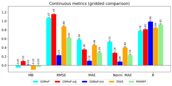
Figure 4.
Gridded comparison metrics. Mean bias (MB), root-mean-squared-error (RMSE), mean absolute error (MAE), normalized mean absolute error (Norm. MAE) and Pearson Correlation coefficient are shown. The units of MB, RMSE and MAE are in mm/day, while Norm. MAE and R are unitless.
AGCD was chosen as truth as it is the operational dataset being used by the BOM in addition to it having performed the best in the point validation. It should be noted that AGCD has its own biases, especially in gauge-sparse regions. Additionally, the use of AGCD both as truth as well as a component in GSMaP-bld means that GSMaP-bld could benefit from in-sample skill inflation. These two factors were addressed in Section 2.4.
GSMaP-adj showed an inferior MB and RMSE compared to GSMaP, with the MB indicating a larger overall positive bias. However, the MAE, normalized MAE and R were superior. The discrepancy stems from how the adjustment process over-adjusted a relatively small number of totals, especially over western Tasmania. These errors in the large totals result in the RMSE showing a different trend to the MAE and the normalized MAE, as the RMSE is more sensitive to large errors. The adjustment process also involved a greater degree of upwards adjustment than downwards adjustment. GSMaP-adj showed comparable performance to ERA5, while GSMaP-bld clearly showed superior performance. MSWEP performed well relatively again.
Compared to when the station gauges were used as truth, all the metrics indicated an improvement in performance for the blending process, with the magnitude of improvement being more significant than in the point validation. For example, the MAE and normalized MAE of GSMaP-bld decreased from 0.3 mm/day and 0.17 to 0.10 mm/day and 0.09, respectively. This was expected, as comparing the satellite datasets which are gridded to another gridded dataset greatly reduces the effect of spatial representation errors.
3.2.2. Intensity Analysis
The residuals of the datasets against AGCD were plotted with respect to the gauge totals and shown in Figure 5.
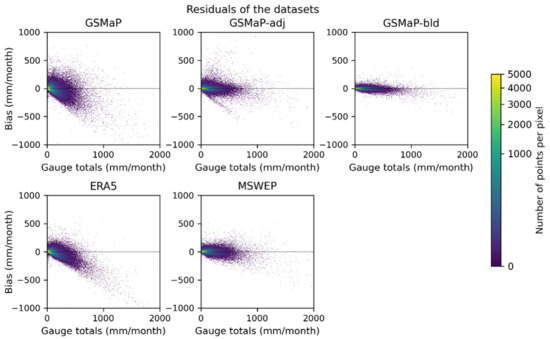
Figure 5.
Residuals of the gridded comparison datasets using AGCD as truth against gauge totals. The shading indicates the number of points in a pixel, allowing the density of the scatterplot to be appreciated. The cube root scale is used.
In line with the general validation, the size of the residuals was smaller when AGCD was used as the truth compared to station data (residuals against station data not shown for brevity). The negative (positive) bias for low (high) totals was much less, though it still existed. This bias was the most noticeable in GSMaP and ERA5, where the underestimation of high-end totals was particularly significant. The over-adjustment in GSMaP-adj was also clearly displayed. GSMaP-bld was the most consistent across the intensities, followed by MSWEP, though both still underestimated high-end totals. The adjustment process was most effective in reducing high-end bias, while the blending process was effective in reducing bias across all intensities.
3.2.3. Spatial and Seasonal Analysis
The mean bias against AGCD for the datasets across the seasons is spatially depicted in Figure 6.
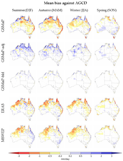
Figure 6.
Mean bias of datasets categorized by seasons using AGCD as truth.
GSMaP had a wet bias along the far northern tropical coastline of Australia but generally a dry bias elsewhere, especially over inland northern Australia, along the GDR and western Tasmania. ERA5 had a dry bias over inland northern Australia and western Tasmania, but a wet bias along the GDR. The bias over western Tasmania was likely a result of lower rain gauge density combined with the high heterogeneity of rainfall due to orography over this region. MSWEP had reduced biases over Tasmania but retained a wet bias over the GDR and a dry bias over the tropical north-west of Australia. Spring showed the greatest difference in bias to the other seasons, a result of rainfall being seasonally lower.
The adjustment process was effective in reducing the dry bias in GSMaP, but over-adjustment resulted in the area and magnitude of the wet bias increasing, particularly during the wet season in northern Australia, where rainfall totals are naturally substantial. The greatest improvement was over Western Tasmania, where the bias was reduced across all seasons. The improvement was also significant over the south-east and east coast. The adjustment process appears to be more useful where stations exist. This can explain the more notable reduction in errors along the densely populated eastern coastlines.
The blending process improved upon GSMaP-adj by reducing much of both the induced and existing wet biases, especially over the northern coastline. The dry bias over Western Tasmania was also improved. It should be noted that because AGCD was used to create GSMaP-bld, a lower bias compared to the other datasets would be expected, given its shared use as truth. However, there are differences over inland northern Australia and particularly a wet bias patch in winter over the inland north-east of Western Australia. This wet bias patch is notable as it is likely related to GSMaP-bld representing missed rainfall over this region during winter.
Figure 7 shows the MB, MAE and R over the individual months of the verification period.
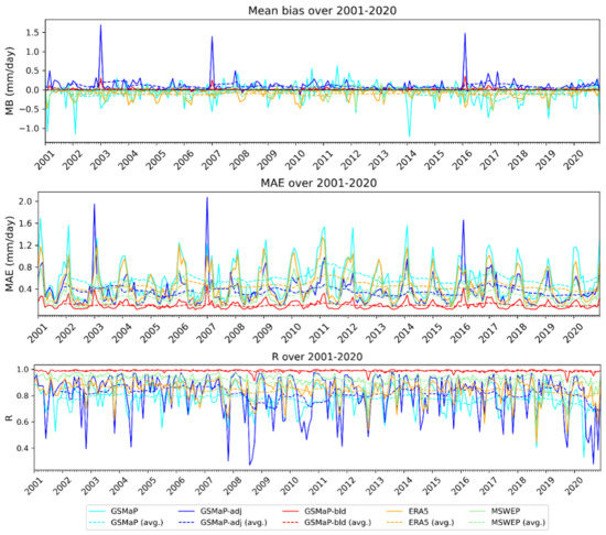
Figure 7.
Time series of the metrics from the gridded comparison. Mean bias (MB), mean absolute error (MAE) and Pearson correlation coefficient using AGCD as truth are shown.
GSMaP-bld was again consistently the best performing dataset. ERA5 and GSMaP showed a more pronounced negative bias during the wet season. A 12-month rolling average is also depicted, showing that the performance of the datasets does not demonstrate a noticeable trend over the validation period.
In general, GSMaP-bld performed the best, followed by MSWEP, then by either GSMaP-adj or ERA5, with GSMaP performing the worse. There were exceptions to this, such as in January 2003, when an over-adjustment of rainfall over northern Australia led to GSMaP-adj being the worst dataset by far for that month.
The variance in R for GSMaP and GSMaP-adj was due to the degree of disagreement in rainfall areas with AGCD. This occurred when GSMaP contains areas of low rainfall where the AGCD dataset had none. The adjustment process cannot void these rainfall areas, as it only adjusts the magnitude and, in some cases, even upwards. As a result, the correlation statistic of GSMaP and GSMaP-adj was low in these months, but since the rainfall totals in these areas were small, the error was not substantial and the bias statistics were more acceptable.
3.2.4. Spread and Extremes Analysis
The CV of all the datasets along with the bottom and top quintile hit rates of the datasets are shown in Figure 8.
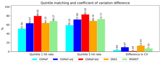
Figure 8.
Spread metrics for the datasets used in the gridded comparison.
The adjustment and blending process were effective in increasing the similarity of the bottom and top quintiles to AGCD. ERA5 has a lower quintile 1 hit rate than GSMaP, suggesting it did not capture the occurrence of low-end totals as well as GSMaP. This could be from spurious precipitation. All the datasets had higher CVs than AGCD, though the difference in the case of GSMaP-bld was only slight.
ERA5 had the largest CV, which is related to it having the lowest mean across the datasets along with a low standard deviation. MSWEP had relatively good quintile hit rates but a relatively high difference in the CV due to a low mean and standard deviation. Consideration of these findings suggests both MSWEP and ERA5 have distributions that are too tight. GSMaP-adj had a greater difference in the CV than GSMaP-bld as well, stemming from high-end totals being exaggerated in comparison to the rest of the population. GSMaP-bld appeared to have the closest statistics to AGCD in terms of quintile matching and spread, as indicated by the CV.
3.3. Visual Inspection Comparison
The data for all the months were plotted and inspected visually to identify patterns of interest. This section presents the driest and wettest months from the validation period as well as the selection of a month that illustrates a recurring pattern evident across the period. The two extreme months were chosen to illustrate two very different rainfall scenarios. The data visualized is GSMaP, GSMaP-bld, MSWEP and AGCD to demonstrate how the full process improved the original data as well as how the final blended product compares to two other established datasets. Differences against AGCD are presented in Appendix C, while a comparison of annual averages during the study period is included in Appendix D. Figure 9 illustrates the totals for September 2018, the driest month in this study period and the second driest month (and the driest September) since records began in 1900 [51]. Dry conditions for this month were associated with cool sea surface temperatures in the eastern Indian Ocean, leading to a reduction in available moisture for precipitation over Australia [51].
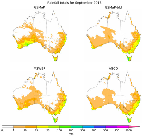
Figure 9.
Rainfall totals for GSMaP, GSMaP-bld, MSWEP and AGCD for September 2018.
The datasets had similar patterns of rainfall, with large parts of the country being dry. The similarity was greater for GSMaP-bld, AGCD and MSWEP. There were also slight discrepancies with rainfall over central Australia, though these totals were small. MSWEP possessed some additional rainfall in southern Western Australia, which could be legitimate given the low rain gauge density over this area. Figure 10 illustrates the totals for March 2011, the wettest month in this study period and the fourth wettest month (and the wettest March) on record [52]. Increased moisture over Australia was associated with a decaying La Niña event, with the country being impacted by a very active monsoon trough over northern Australia and a series of low-pressure troughs over eastern Australia [52].
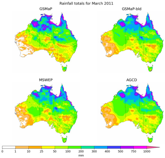
Figure 10.
Rainfall totals for GSMaP, GSMaP-bld, MSWEP and AGCD during March 2011.
The pattern was again consistent for most parts of the country though there were a few key differences. The first was over north-eastern Western Australia where GSMaP-bld had a small strip of rainfall greater than MSWEP or AGCD. It is likely the rainfall in this region is legitimate but was missed in AGCD as it corresponds to a region that has no nearby rain gauges. In MSWEP and GSMaP-bld, there was also a notable rainfall ‘bullseye’ around the junction of Northern Territory, Queensland and South Australia which was not present in AGCD. This is another region that does not possess rain gauges.
Inspection of all the months strongly reinforces the observation that the greatest value of GSMaP-bld is obtained when there is significant rainfall over areas where there are no rain gauges. These scenarios were most common over the interior of Western Australia and western South Australia, where the rain gauge density is the lowest. The blending technique was able to capture what appears to be missed rainfall in these areas but was more effective over the northern interior of Western Australia than the southern interior. As an example, Figure 11 illustrates this wherein July 2001 a band of increased rainfall over the northern interior of WA was represented in both GSMaP-bld and MSWEP but not AGCD.
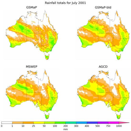
Figure 11.
Rainfall totals for GSMaP, GSMaP-bld, MSWEP and AGCD during July 2011.
4. Discussion
The results demonstrated that there are regions where corrected satellite data could improve a pure station-based analysis and that a product that blended satellites and rain gauge data could exhibit superior performance to the individual datasets themselves.
The blending process appears to be most beneficial between late austral autumn and early spring. This is likely in part due to the correction of known deficiencies of satellites over the austral winter period, including the capturing of rainfall from frontal systems and low clouds [9], as well as rectifying snow contamination [35]. The fact that the errors in the blended dataset do not have a distinct seasonality indicates that the blending process was valuable in eliminating this form of bias which otherwise would have manifested as a distinct seasonal trend. The residual bias was more likely to be from differences away from gauges that were not necessarily linked to the seasons.
From a cursory glance, the results of the gridded validation suggested the adjustment process may not have been effective, as although the MAE decreased and the R increased, there were also increases in the RMSE and MB. This was due to the over-adjustment of a relatively small number of high rainfall totals, especially over western Tasmania, that skewed these bias statistics, even though the overall effect was valuable. The over-adjustment can be attributed to multiple reasons. The first was that areal averages were adjusted to point totals. Point totals will generally be greater than their areal averages and so this adjustment would lead to a positive bias, especially if there are only a few stations in a grid point. Secondly, the number of stations over which GSMaP had a negative bias could span a substantial area. This resulted in an indiscriminately widespread upwards adjustment to totals around these stations, resulting in broad over-adjustment. An example of this occurred in January 2003 over the northern tropics of Australia.
Another factor was the appearance of erroneous ‘bullseyes’ artefacts. This occurred when GSMaP already possessed localized higher areas of rainfall and these ‘bullseyes’ were surrounded by regions where less rainfall had been detected by the rain gauges relative to GSMaP. The result of the adjustment process was to increase rainfall over these regions, leading to the ‘bullseyes’ becoming much larger than the gauge-based datasets as well as ERA5 and MSWEP. An example of this occurred during March 2009 in Western Australia.
The combination of both of these factors can explain the systematic over-adjustment of rainfall (both in magnitude and extent) over Western Tasmania, where gauge rainfall is consistently and significantly greater than GSMaP. Clipping the adjustment ratio to a lower number should generally improve the adjustment process, though care has to be taken to ensure appropriate high-end adjustments are still possible.
Even though there are problems with the adjustment process, especially for high-end totals, the step is still important, as seen by the marked drop in performance of the blended dataset if the adjustment was not performed as an intermediary step. Nonetheless, the blending process is critical in further reducing the biases in GSMaP-adj, as well as correcting any induced artefacts. Ultimately this highlights that the adjustment and raw blending processes are limited in performance when implemented in isolation but markedly more robust when they are combined.
Inspection of the rainfall patterns in Section 3.3 revealed the blended dataset has great value in poorly observed areas where the gauge analysis can commonly miss significant rainfall due to a complete absence of rain gauges. Northern Western Australia in particular benefitted from the more realistic pattern depicted in GSMaP-bld. In addition to poorly observed areas, areas where rainfall has high spatiotemporal variation such over topography also greatly improved because of the blending and adjustment processes. GSMaP severely underestimated rainfall over topography. This is a systematic bias in satellite rainfall estimates due to the difficulty they have with the detection of the relatively warm clouds associated with orographic rainfall [34]. The blending process was very valuable in correcting this effect where there was sufficient rain gauge density, as shown over western Tasmania. The adjustment process over-adjusted the values, but the blending process corrected this, as well as existing wet biases over northern Australia, to consistently result in much more accurate totals.
There were cases where realistic patterns of rainfall in GSMaP were lost due to the blending process, with the final result looking more akin to AGCD. In some cases, this was because the rainfall was not replicated in MSWEP (used as the reference in the blending process) and, consequently, GSMaP-adj was not given a proper weighting. On other occasions, GSMaP was over-adjusted, and so, when it was compared to MSWEP, its error variance was high and, accordingly, its weight was low. In terms of poorly observed areas, this seemed to occur less over northern Western Australia than in other parts of central Australia.
The north-western part of Western Australia is an area where AGCD is likely to possess greater error given the reduced rain gauge density, especially inland of the coast. Compared to the non-gauge-based datasets, AGCD is wetter, which could be a result of isolated totals over rain gauges being incorrectly interpolated over a broader area. The use of a climatological floor in AGCD (the background field is floored at 2 mm) [27] could be another reason why a positive bias is present, especially over areas with climatologically-low rainfall totals. It is likely to be appropriate if GSMaP-bld could retain lower totals over this region too, but the blending process removed much of this effect, with only a weak dry bias remaining.
Alternative adjustment methods can be explored. Quintile-to-quintile matching is employed in GSMaP and CMORPH to correct biases and would help to remove the incongruity from the direct matching of areal averages to point totals in the current process [19,26]. If a more accurate GSMaP-adj can be made, this will yield better weights for it during the blending process, allowing its advantage over gauge observations to be better exhibited in poorly observed areas. Another way to provide greater weighting to the satellite datasets in poorly observed areas is to directly include gauge density in the weights, such as through the use of empirical relationships.
Methods of interpolating the point values other than ordinary kriging should also be investigated. Ordinary kriging assumes a constant mean and variogram across the entire domain. In reality, these assumptions will not hold in many areas such as where the error in rainfall is impacted by other spatial influences such as topography.
Future research will investigate other adjustment methods, in addition to alternative interpolation methods such as other variants of kriging, or optimal interpolation using the satellite rainfall as a first guess field.
5. Conclusions
Gridded rainfall data provides a spatially consistent representation of rainfall over an area, but the accuracy of analyses based on rain gauges is reduced over areas with no rain gauges. In the case of Australia, there are large gaps in the station network over central Australia, which the operational rainfall analysis AGCD can fail to represent accurately. In this study, a technique for blending AGCD with GSMaP satellite data using a two-step approach was developed. The first step corrected GSMaP to rain gauge data using multiplicative ratios that were converted to a grid using ordinary kriging. The second step blended the adjusted GSMaP data with AGCD using an inverse error variance weighting method, with MSWEP used as a reference.
Data validation was performed over 20 years from 2001 to 2020 and the results showed that the method was successful, creating a dataset that had better accuracy over stations than other non-gauge-based analyses. The greatest reduction in biases was obtained from extreme totals and over regions with topography, provided the rain gauge density was sufficient. Importantly, the blended dataset also had a more realistic representation of rainfall over data-sparse areas than AGCD. Further research will be valuable in refining this method with a more effective adjustment scheme being an important objective. One of the advantages of this method is its transferability to other regions, but its regional effectiveness cannot be generalized and so its performance in other regions, especially where the rain gauge density is lower, is also another important future consideration.
Author Contributions
Conceptualization, Z.-W.C., Y.K., A.B.W., S.C. and C.S.; methodology, Z.-W.C., Y.K., S.C. and C.S.; software, Z.-W.C.; validation, Z.-W.C.; formal analysis, Z.-W.C.; investigation, Z.-W.C.; resources, Z.W-C. and Y.K.; data curation, Z.-W.C. and Y.K.; writing—original draft preparation, Z.-W.C.; writing—review and editing, Z.-W.C., Y.K., A.B.W., S.C. and C.S.; visualization, Z.-W.C.; supervision, Y.K., A.B.W., S.C. and C.S.; project administration, Y.K.; funding acquisition, Y.K. All authors have read and agreed to the published version of the manuscript.
Funding
This research was supported by the World Meteorological Organization through “Weather and Climate Early Warning System for Papua New Guinea (CREWS-PNG)” project 20170888.
Data Availability Statement
GSMaP data were provided by EORC, JAXA and can be obtained by registering as a user at https://sharaku.eorc.jaxa.jp/GSMaP/index.htm, accessed on 16 February 2022. CMORPH data were provided by CPC, NOAA and can be obtained at https://ftp.cpc.ncep.noaa.gov/precip/PORT/SEMDP/CMORPH_BLD/DATA/, accessed on 16 February 2022. AGCD and station gauge data were provided by the Bureau of Meteorology and can be obtained from http://dx.doi.org/10.25914/6009600786063, accessed on 16 February 2022. This research contains modified Copernicus Climate Change Service Information (2019) due to use of ERA5 data which can be obtained from https://cds.climate.copernicus.eu/cdsapp#!/dataset/reanalysis-era5-single-levels-monthly-means, accessed on 16 February 2022. Neither the European Commission nor the ECMWF is responsible for any use that may be made of the Copernicus Information or data it contains. MSWEP data were provided by GloH2O, which can be obtained by seeking permission from http://www.gloh2o.org/mswep/, accessed on 16 February 2022.
Acknowledgments
We are grateful to colleagues from the Climate Monitoring and Long-Range Forecasts sections of the Bureau of Meteorology for their helpful advice and guidance and to the anonymous reviewers who provided valuable comments which helped us to improve the quality of the initial manuscript.
Conflicts of Interest
The authors declare no conflict of interest.
Appendix A
Various GSMaP-adj datasets were created by varying the variogram model used in the kriging process of the ratio grids. The variogram models trialed were those based on linear, power, Gaussian, spherical and exponential equations with the comparison to gauge data shown in Figure A1.
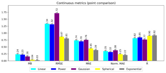
Figure A1.
Gridded comparison of different variogram models using AGCD as truth. Mean bias (MB), root-mean-squared-error (RMSE), mean absolute error (MAE), normalized mean absolute error (Norm. MAE) and Pearson correlation coefficient (R) are shown. The units of MB, RMSE and MAE are in mm/day, while Norm. MAE and R are unitless.
The Gaussian model was the worst, followed by the linear and power models. Under a Gaussian model, the slope of the variogram is less steep near the origin (i.e., the variance increases slower) than the other models, suggesting a greater degree of continuity and local correlation which did not seem to be as appropriate for modelling the satellite error as the other models. Using the spherical and exponential models resulted in the best performance, with the exponential model displaying the best metrics.
Compared to the spherical model, the exponential model has a steeper slope near the origin. The spherical model also reaches the sill after a finite range, indicating there is a distance where the sampled points cease to have an influence while the exponential model is asymptotic towards the sill. Given the results of the comparison, the exponential model was chosen for the adjustment process.
Appendix B
Comparison of the error variances for GSMaP-adj and AGCD against MSWEP facilitates an analysis of where GSMaP-adj is able to outperform AGCD and to what degree. Figure A2 shows the difference between the error variance of GSMaP-adj and AGCD categorized by the months of the year.
It shows that although AGCD was superior to GSMaP-adj in the majority of areas and times of the year, there were cases where GSMaP-adj exhibited a comparable or even smaller error variance than AGCD. Many of these patches are over central Australia where there is low rain gauge density and satellite data is expected to have an advantage over interpolated gauge data. For example, swathes in eastern Western Australia, northern South Australia and southern Northern Territory exhibit a lower error variance for GSMaP-adj compared to AGCD for many months of the year.
During the austral winter months from June to August, GSMaP-adj also had a comparable performance to AGCD across large parts of northern Australia. This is likely in part due to the low rainfall totals experienced in these regions over this period. AGCD consistently outperformed GSMaP-adj over western Tasmania and there was a large error in GSMaP-adj over northern Australia during the summer.
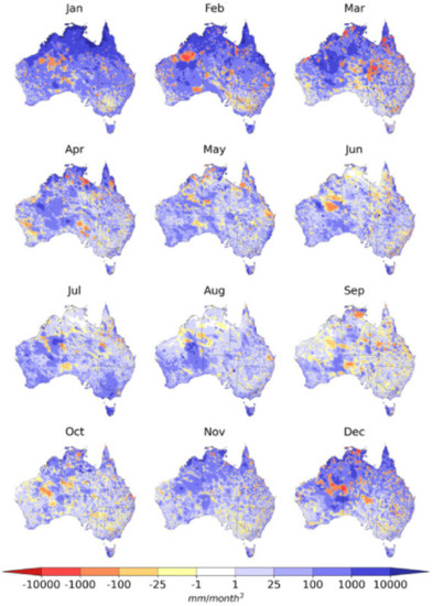
Figure A2.
Difference between error variance of GSMaP-adj and AGCD against MSEP. Negative (positive) values indicate GSMaP-adj (AGCD) is better than its counterpart.
Appendix C
The differences in the monthly totals for September 2018, March 2011 and July 2001 are shown in Figure A3.
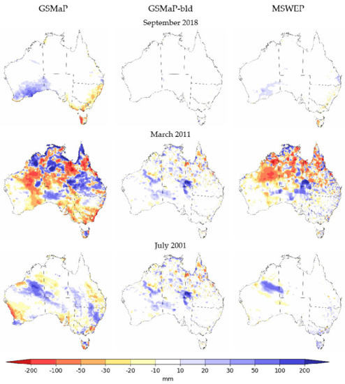
Figure A3.
Difference in monthly totals to AGCD.
Appendix D
The average annual rainfall over the study period of 2000 to 2001 for GSMaP, GSMaP-bld, AGCD and MSWEP are visualized for comparison purposes in Figure A4.
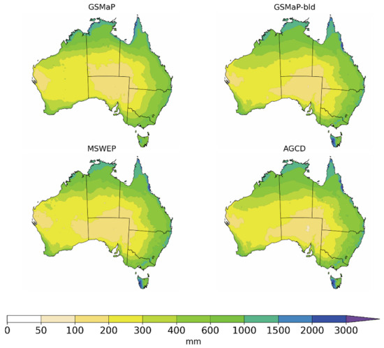
Figure A4.
Average annual rainfall totals for GSMaP, GSMaP-bld, MSWEP and AGCD for the period 2001 to 2020.
Representations of the average annual totals are similar on a large-scale between the datasets. Key improvements visible in GSMaP-bld over GSMaP are increased rainfall along the Queensland coast, over the Great Dividing Range and over Western Tasmania, in addition to a reduction in rainfall over the southeast interior of Western Australia. AGCD depicts less rainfall than GSMaP-bld over a region in north-west South Australia; this region has low gauge density, and so it is reasonable to infer that AGCD may be incorrectly underestimating rainfall over this area.
References
- Kidd, C.; Huffman, G. Global precipitation measurement. Meteorol. Appl. 2011, 18, 334–353. [Google Scholar] [CrossRef]
- Koch, S.E.; Desjardins, M.; Kocin, P.J. An interactive Barnes objective map analysis scheme for use with satellite and conventional data. J. Clim. Appl. Meteorol. 1983, 22, 1487–1503. [Google Scholar] [CrossRef]
- Jones, D.A.; Wang, W.; Fawcett, R. High-quality spatial climate data-sets for Australia. Aust. Meteorol. Oceanogr. J. 2009, 58, 233–248. [Google Scholar] [CrossRef]
- Kidd, C.; Becker, A.; Huffman, G.J.; Muller, C.L.; Joe, P.; Skofronick-Jackson, G.; Kirschbaum, D.B. So, how much of the Earth’s surface is covered by rain gauges? Bull. Am. Meteorol. Soc. 2017, 98, 69–78. [Google Scholar] [CrossRef] [PubMed]
- Michaelides, S.; Levizzani, V.; Anagnostou, E.; Bauer, P.; Kasparis, T.; Lane, J.E. Precipitation: Measurement, remote sensing, climatology and modeling. Atmos. Res. 2009, 94, 512–533. [Google Scholar] [CrossRef]
- Michelson, D.B. Systematic correction of precipitation gauge observations using analyzed meteorological variables. J. Hydrol. 2004, 290, 161–177. [Google Scholar] [CrossRef]
- Peterson, T.C.; Easterling, D.R.; Karl, T.R.; Groisman, P.; Nicholls, N.; Plummer, N.; Torok, S.; Auer, I.; Boehm, R.; Gullet, D.; et al. Homogeneity adjustments of in situ atmospheric climate data: A review. Int. J. Climatol. 1998, 18, 1493–1517. [Google Scholar] [CrossRef]
- Groisman, P.Y.; Legates, D.R. The accuracy of United States precipitation data. Bull. Am. Meteorol. Soc. 1994, 75, 215–227. [Google Scholar] [CrossRef]
- Ebert, E.E.; Janowiak, J.E.; Kidd, C. Comparison of near-real-time precipitation estimates from satellite observations and numerical models. Bull. Am. Meteorol. Soc. 2007, 88, 47–64. [Google Scholar] [CrossRef] [Green Version]
- Kummerow, C.; Giglio, L. A passive microwave technique for estimating rainfall and vertical structure information from space. Part I: Algorithm description. J. Appl. Meteorol. 1994, 33, 3–18. [Google Scholar] [CrossRef]
- Beck, H.E.; Vergopolan, N.; Pan, M.; Levizzani, V.; Van Dijk, A.I.J.M.; Weedon, G.P.; Brocca, L.; Pappenberger, F.; Huffman, G.J.; Wood, E.F. Global-scale evaluation of 22 precipitation datasets using gauge observations and hydrological modeling. Hydrol. Earth Syst. Sci. 2017, 21, 6201–6217. [Google Scholar] [CrossRef] [Green Version]
- Jiang, Q.; Li, W.; Wen, J.; Fan, Z.; Chen, Y.; Scaioni, M.; Wang, J. Evaluation of satellite-based products for extreme rainfall estimations in the eastern coastal areas of China. J. Integr. Environ. Sci. 2019, 16, 191–207. [Google Scholar] [CrossRef] [Green Version]
- Ali, G.; Sajjad, M.; Kanwal, S.; Xiao, T.; Khalid, S.; Shoaib, F.; Gul, H.N. Spatial–temporal characterization of rainfall in Pakistan during the past half-century (1961–2020). Sci. Rep. 2021, 11, 1–15. [Google Scholar] [CrossRef]
- Verdin, A.; Rajagopalan, B.; Kleiber, W.; Funk, C. A Bayesian kriging approach for blending satellite and ground precipitation observations. Water Resour. Res. 2015, 51, 908–921. [Google Scholar] [CrossRef]
- Frazier, A.G.; Giambelluca, T.W.; Diaz, H.F.; Needham, H.L. Comparison of geostatistical approaches to spatially interpolate month-year rainfall for the Hawaiian Islands. Int. J. Climatol. 2016, 36, 1459–1470. [Google Scholar] [CrossRef] [Green Version]
- Lin, A.; Wang, X.L. An algorithm for blending multiple satellite precipitation estimates with in situ precipitation measurements in Canada. J. Geophys. Res. Atmos. 2011, 116, D21111. [Google Scholar] [CrossRef] [Green Version]
- Adhikary, S.K.; Muttil, N.; Yilmaz, A.G. Cokriging for enhanced spatial interpolation of rainfall in two Australian catchments. Hydrol. Process. 2017, 31, 2143–2161. [Google Scholar] [CrossRef] [Green Version]
- Chappell, A.; Renzullo, L.H.; Raupach, T.J.; Haylock, M. Evaluating geostatistical methods of blending satellite and gauge data to estimate near real-time daily rainfall for Australia. J. Hydrol. 2013, 493, 105–114. [Google Scholar] [CrossRef]
- Xie, P.; Xiong, A.Y. A conceptual model for constructing high-resolution gauge-satellite merged precipitation analyses. J. Geophys. Res. Atmos. 2011, 116, D21106. [Google Scholar] [CrossRef]
- Chua, Z.W.; Kuleshov, Y.; Watkins, A.B. Drought detection over papua new guinea using satellite-derived products. Remote Sens. 2020, 12, 3859. [Google Scholar] [CrossRef]
- National Centers for Environmental Information, National Geophysical Data Center. ETOPO1 Global Relief | National Centers for Environmental Information. Available online: https://www.ngdc.noaa.gov/mgg/global/ (accessed on 16 November 2020).
- Bureau of Meteorology. Australian Climate Averages-Climate Classifications. Available online: http://www.bom.gov.au/jsp/ncc/climate_averages/climate-classifications/index.jsp (accessed on 16 February 2022).
- Australian Climate Averages. Rainfall (Climatology 1981–2010). Available online: http://www.bom.gov.au/jsp/ncc/climate_averages/rainfall/index.jsp?period=an&area=vc#maps (accessed on 16 February 2022).
- Tashima, T.; Kubota, T.; Mega, T.; Ushio, T.; Oki, R. Precipitation Extremes Monitoring Using the Near-Real-Time GSMaP Product. IEEE J. Sel. Top. Appl. Earth Obs. Remote Sens. 2020, 13, 5640–5651. [Google Scholar] [CrossRef]
- Chua, Z.W.; Kuleshov, Y.; Watkins, A. Evaluation of satellite precipitation estimates over Australia. Remote Sens. 2020, 12, 678. [Google Scholar] [CrossRef] [Green Version]
- Mega, T.; Ushio, T.; Matsuda, T.; Kubota, T.; Kachi, M.; Oki, R. Gauge-Adjusted Global Satellite Mapping of Precipitation. IEEE Trans. Geosci. Remote Sens. 2019, 57, 1928–1935. [Google Scholar] [CrossRef]
- Evans, A.; Jones, D.; Smalley, R.; Lellyett, S. An Enhanced Gridded Rainfall Dataset Scheme for Australia; Bureau of Meteorlogy: Melbourne, Australia, 2020; ISBN 978-1-925738-12-4.
- Beck, H.E.; Wood, E.F.; Pan, M.; Fisher, C.K.; Miralles, D.G.; Van Dijk, A.I.J.M.; McVicar, T.R.; Adler, R.F. MSWep v2 Global 3-hourly 0.1° precipitation: Methodology and quantitative assessment. Bull. Am. Meteorol. Soc. 2019, 100, 473–500. [Google Scholar] [CrossRef] [Green Version]
- Hersbach, H.; Bell, B.; Berrisford, P.; Hirahara, S.; Horányi, A.; Muñoz-Sabater, J.; Nicolas, J.; Peubey, C.; Radu, R.; Schepers, D.; et al. The ERA5 global reanalysis. Q. J. R. Meteorol. Society. 2020, 146, 1999–2049. [Google Scholar] [CrossRef]
- A Draft Document Prepared for Cli-Manage 2000 Australian Data Archive Australian Data Archive for Meteorology for Meteorology; Australian Data Archive for Meteorology for Meteorology: Melbourne, Australia, 2000.
- Tang, G.; Clark, M.P.; Papalexiou, S.M.; Ma, Z.; Hong, Y. Have satellite precipitation products improved over last two decades? A comprehensive comparison of GPM IMERG with nine satellite and reanalysis datasets. Remote Sens. Environ. 2020, 240, 111697. [Google Scholar] [CrossRef]
- Shen, Z.; Yong, B.; Yi, L.; Wu, H.; Xu, H. From TRMM to GPM, how do improvements of post/near-real-time satellite precipitation estimates manifest? Atmos. Res. 2022, 268, 106029. [Google Scholar] [CrossRef]
- Derin, Y.; Yilmaz, K.K. Evaluation of multiple satellite-based precipitation products over complex topography. J. Hydrometeorol. 2014, 15, 1498–1516. [Google Scholar] [CrossRef] [Green Version]
- Dinku, T.; Ceccato, P.; Grover-Kopec, E.; Lemma, M.; Connor, S.J.; Ropelewski, C.F. Validation of satellite rainfall products over East Africa’s complex topography. Int. J. Remote Sens. 2007, 28, 1503–1526. [Google Scholar] [CrossRef]
- Stampoulis, D.; Anagnostou, E. Evaluation of global satellite rainfall products over Continental Europe. J. Hydrometeorol. 2012, 13, 588–603. [Google Scholar] [CrossRef]
- Ning, S.; Song, F.; Udmale, P.; Jin, J.; Thapa, B.R.; Ishidaira, H. Error Analysis and Evaluation of the Latest GSMap and IMERG Precipitation Products over Eastern China. Adv. Meteorol. 2017, 2017, 1–16. [Google Scholar] [CrossRef] [Green Version]
- Habib, E.; Haile, A.T.; Tian, Y.; Joyce, R.J. Evaluation of the high-resolution CMORPH satellite rainfall product using dense rain gauge observations and radar-based estimates. J. Hydrometeorol. 2012, 13, 1784–1798. [Google Scholar] [CrossRef]
- Karaseva, M.O.; Prakash, S.; Gairola, R.M. Validation of high-resolution TRMM-3B43 precipitation product using rain gauge measurements over Kyrgyzstan. Theor. Appl. Climatol. 2012, 108, 147–157. [Google Scholar] [CrossRef]
- Fitzjarrald, D.R.; Sakai, R.K.; Moraes, O.L.L.; De Oliveira, R.C.; Acevedo, O.C.; Czikowsky, M.J.; Beldini, T. Spatial and temporal rainfall variability near the amazon-tapajós confluence. J. Geophys. Res. Biogeosci. 2008, 113, G00B11-n/a. [Google Scholar] [CrossRef]
- Guo, H.; Bao, A.; Ndayisaba, F.; Liu, T.; Kurban, A.; De Maeyer, P. Systematical Evaluation of Satellite Precipitation Estimates Over Central Asia Using an Improved Error-Component Procedure. J. Geophys. Res. Atmos. 2017, 122, 10,906–10,927. [Google Scholar] [CrossRef]
- Ensor, L.A.; Robeson, S.M. Statistical characteristics of daily precipitation: Comparisons of gridded and point datasets. J. Appl. Meteorol. Climatol. 2008, 47, 2468–2476. [Google Scholar] [CrossRef]
- Pfeifroth, U.; Mueller, R.; Ahrens, B. Evaluation of satellite-based and reanalysis precipitation data in the tropical pacific. J. Appl. Meteorol. Climatol. 2013, 52, 634–644. [Google Scholar] [CrossRef]
- Beck, H.E.; Pan, M.; Roy, T.; Weedon, G.P.; Pappenberger, F.; Van Dijk, A.I.J.M.; Huffman, G.J.; Adler, R.F.; Wood, E.F. Daily evaluation of 26 precipitation datasets using Stage-IV gauge-radar data for the CONUS. Hydrol. Earth Syst. Sci. 2019, 23, 207–224. [Google Scholar] [CrossRef] [Green Version]
- Amjad, M.; Yilmaz, M.T.; Yucel, I.; Yilmaz, K.K. Performance evaluation of satellite- and model-based precipitation products over varying climate and complex topography. J. Hydrol. 2020, 584, 124707. [Google Scholar] [CrossRef]
- Hofstra, N.; Haylock, M.; New, M.; Jones, P.; Frei, C. Comparison of six methods for the interpolation of daily, European climate data. J. Geophys. Res. Atmos. 2008, 113, D21. [Google Scholar] [CrossRef] [Green Version]
- Huffman, G.J.; Adler, R.F.; Arkin, P.; Chang, A.; Ferraro, R.; Gruber, A.; Janowiak, J.; McNab, A.; Rudolf, B.; Schneider, U. The Global Precipitation Climatology Project (GPCP) Combined Precipitation Dataset. Bull. Am. Meteorol. Soc. 1997, 78, 5–20. [Google Scholar] [CrossRef]
- Vila, D.A.; de Goncalves, L.G.G.; Toll, D.L.; Rozante, J.R. Statistical evaluation of combined daily gauge observations and rainfall satellite estimates over continental South America. J. Hydrometeorol. 2009, 10, 533–543. [Google Scholar] [CrossRef]
- Gumindoga, W.; Rientjes, T.H.M.; Tamiru Haile, A.; Makurira, H.; Reggiani, P. Performance of bias-correction schemes for CMORPH rainfall estimates in the Zambezi River basin. Hydrol. Earth Syst. Sci. 2019, 23, 2915–2938. [Google Scholar] [CrossRef] [Green Version]
- Kumar Adhikary, S.; Muttil, N.; Gokhan Yilmaz, A. Ordinary kriging and genetic programming for spatial estimation of rainfall in the Middle Yarra River catchment, Australia. Hydrol. Res. 2016, 47, 1182–1197. [Google Scholar] [CrossRef]
- Wackernagel, H. Multivariate geostatistics: An introduction with applications. Multivar. Geostat. Introd. Appl. 1995, 91, 79–97. [Google Scholar] [CrossRef]
- Special Climate Statement 66-an Abnormally Dry Period in Eastern Australia; Bureau of Meteorology: Melbourne, Australia, 2018.
- Special Climate Statement 31-Wettest March on Record in Australia; Bureau of Meteorology: Melbourne, Australia, 2011.
Publisher’s Note: MDPI stays neutral with regard to jurisdictional claims in published maps and institutional affiliations. |
© 2022 by the authors. Licensee MDPI, Basel, Switzerland. This article is an open access article distributed under the terms and conditions of the Creative Commons Attribution (CC BY) license (https://creativecommons.org/licenses/by/4.0/).