1. Introduction
Land cover information is paramount for a wide range of applications, such as spatial planning and environmental monitoring, which consider land cover patterns and dynamics to regulate human activities and assess or predict their impacts [
1,
2]. Land cover is also a very important theme in a spectrum of scientific fields, for example to understand fundamental interactions between the atmosphere and land and their impact on climate and biodiversity [
3,
4]. Demand for land cover information is therefore large and has increased considerably in recent decades as societies become more complex and technology and science evolve.
Land cover maps have been produced in a variety of settings [
5], and some of them represent a breakthrough in spatial sciences, including remote sensing. Examples include early global land cover maps [
6] and map series from operational mapping programmes (e.g., CORINE Land Cover). These maps play a very important role in science, society, and policy, but are subject to the criticism of being insufficient to respond conveniently to the needs of all users of land cover information. For example, global maps are historically associated with low spatial resolution and modest thematic accuracy [
7]. Recent improvements in global products are notable [
8,
9], but strong spatial asymmetries in regard to thematic accuracy at regional or national scales have been reported [
9,
10,
11,
12,
13,
14]. Furthermore, thematic detail may be coarse and updates infrequent (e.g., GlobeLand30 is updated every 10 years and includes 10 classes). More localised mapping efforts can overcome some of these issues, but downsides persist. For example, in Europe, CORINE Land Cover (CLC) was started in the 1980s to produce maps in vector format with a minimum mapping unit (MMU) of 25 ha, minimum width of linear elements (MMW) of 100 m, and 44 thematic classes, in most cases interpreted visually from remote sensing data [
15,
16]. The same technical specifications are preserved through map updating every six years for historical consistency, which is an asset for long-term analysis, but a disadvantage for applications requiring fine spatial and temporal detail.
Alternative mapping approaches are needed, and indeed, new developments have prompted new impetus to land cover mapping from remote sensing, including open imagery archives, high-performance computing, and advances in data analysis [
17]. Old constraints on remote sensing data analysis were mitigated and automation has increasingly gained ground in research agendas and practice. Operational methods are being developed that use semi-automatic methods to analyse large volumes of remote sensing data, such as Landsat and Sentinel. For example, in Europe, CLC is currently undergoing a thorough revision and evolving to a “second generation”, called CLC+. The new CLC+ moves away from traditional visual interpretation of remote sensing data and includes advanced image analysis, such as supervised image classification and segmentation [
18]. Other examples include new products and programmes, such as Malinowski et al. [
19], who developed an automatic classification workflow of multi-temporal Sentinel-2 imagery for Europe to produce a map of 13 classes relative to 2017 and envisaging annual updates. Similarly, another map of eight classes relative to 2018 and annually updatable was produced for Europe by Venter and Sydenham [
20] with Sentinel-2 and Sentinel-1 data. LCMAP is a new operational programme of the USA that uses the extensive Landsat archive to detect and classify changes in land cover and produce a suite of 10 annual land cover products [
21]. The European Space Agency (ESA) recently released WorldCover at 10 m resolution and 11 classes for 2020 based on Sentinel-1 and 2 data [
22].
Countries can benefit from upcoming products as new and better maps are expected in the future. Despite that, there is room for undertaking national efforts on land cover mapping that can provide complementary products with different specifications, larger accuracy, and/or updating [
14]. Furthermore, the fluctuation of thematic accuracy commonly observed in land cover maps as a function of space is especially serious across multiple regions in the world. Southern Europe is one of such regions. To mention a few examples, Portugal and Spain are included in a region of 50–60% overall accuracy in Liu et al.’s work [
9], while a mean overall accuracy of 80.0% is reported for the globe. Validation sites at central Portugal and Albania/Greece are classified by Malinowski et al. [
19] with the lowest overall accuracies among all the European countries mapped (67% and 70.8%, respectively), while the overall accuracy of 86.1% was estimated for the entire map. Venter and Sydenham [
20] report a clear north–south pattern in classification accuracy, with the lowest values occurring across Mediterranean countries such as Portugal, Spain, Italy, and Greece.
The examples above struggle to reach high thematic accuracy and detail everywhere. Possible difficulties emerge where landscapes pose particular problems, hence requiring more complex and customised mapping approaches. That may not be possible in large areas, such as continental and global maps, but at national scales it may be feasible [
14]. For example, post-classification analysis can take advantage of local expert knowledge to overcome misclassifications produced by standard supervised image classification [
23].
The Portuguese national mapping agency (DGT—Directorate General for Territory) is preparing the grounds of a future land cover monitoring system called SMOS (
Sistema de Monitorização de Ocupação do Solo) to frequently deliver land cover and land use products for mainland Portugal. SMOS inherits the traditional land use and land cover map of Portugal (COS) produced through manual delineation and labelling of polygons based on visual interpretation of orthophoto maps with centimetric spatial resolution (although automatic processes with satellite data have been introduced [
24]). However, the production of COS is time-consuming and presents some limitations for several applications (e.g., 1 ha MMU), and hence an annual land cover map, called COSsim, based on Sentinel-2 data was initiated. This map includes several differences from current and forthcoming European and global counterparts. One important difference is that the Portuguese map will discriminate the most important tree species. This paper presents the methodology developed to produce a prototype relative to 2018 as the first map of the future annual map series.
The methodology developed includes automatic procedures, such as training data generation and image classification with random forest (RF). RF has been widely used in operational programmes [
19,
20,
25], offering several practical advantages such as robustness to noise in training data [
26]. The methodology also includes spatial stratification and several stages of analysis and mapping. The goal is to adapt and dedicate image classification and post-classification analysis to local conditions and specific problems to overcome shortcomings of automatic image classification. Post-classification analysis affords new means such as expert knowledge of inferring land cover with the purpose of increasing thematic accuracy and detail. Hence, the methodology is flexible and can be adapted by other countries for national or regional land cover land use mapping. A thorough accuracy assessment provides estimates of thematic accuracy across the territory and the mapping stages of analysis to understand the pros and cons of the mapping approach. The new map for 2018 is presented along with new insights on the Portuguese landscape.
2. Portuguese Landscape
Mainland Portugal covers almost 90,000 km2 in the Iberian Peninsula. The climate is temperate and includes Atlantic and Mediterranean influences, resulting in cold and wet winter, and hot and dry summer seasons. The landscape is very diverse and contrasts between the north and south, where Atlantic and Mediterranean climates are, respectively, more pronounced. Higher temperatures and water scarcity are increasingly found in the south, where vegetation greenness is less exuberant. The flat morphology is associated with extensive agriculture and pastures commonly found in agro-forestry systems of low tree density of evergreen oaks (Cork oak and Holm oak). Higher altitudes found in the central and northern regions are commonly associated with small land ownership, familiar agriculture, and pine and eucalyptus forest. Asymmetries between the coast and inland are also evident, such as human presence and large settlements, which are mainly found along the coast, particularly from the capital Lisbon to the north.
A land cover nomenclature was defined to classify the Portuguese landscape and to make the map relevant for a wide range of applications. Several tree species were included as distinct classes to provide large thematic detail in forested areas. The land cover classes were defined to be as compatible as possible with other maps of Portugal, but some classes were adapted or removed according to the technical specifications of the new map. For example, the 10 m pixel size of the map makes the definition of class agro-forestry areas (found in maps such as COS and CLC) inadequate. Here, agro-forestry areas correspond to several other classes at the scale of the pixel, such as agriculture and trees. The nomenclature includes 13 classes (
Table 1).
Less detailed versions of the nomenclature are also considered to represent less detailed thematic maps. The 13 classes are thus organised in a hierarchical nomenclature of three thematic levels (
Table 1). The 13 thematic classes correspond to the most detailed level (level 3). Level 2 merges the tree species into broadleaves and conifers, making a total of nine classes. The coarser thematic level (level 1) includes six classes as it defines just one class for forest trees, and merges shrubland and natural grassland, and wetlands and water.
4. Methodology
4.1. Overview
The methodology relies on a series of divisions in both the spatial and methodological domains. The goal is to adjust mapping to local conditions stemming from the diversity of the landscape and issues commonly found in image classification. Divisions in the spatial domain, commonly called spatial stratification, have been shown to increase the classification accuracy [
39,
40,
41], and the same concept is used here to define spatial strata. In our methodology, these strata include nested substrata organised in hierarchical levels. Strata are analysed independently from each other at the higher level (e.g., different training samples), while nested sublevels can share data but differ in some procedures (e.g., post-classification analysis).
In the methodological domain, stages of analysis are designed to address specific problems or divide complex mapping tasks in several parts, which can also contribute to enhance the classification accuracy [
41,
42]. Therefore, data analysis is implemented through various stages, in which subsequent stages improve the outputs of precedent stages.
The methodology is explained in detail in the forthcoming sections, allowing for its full understanding.
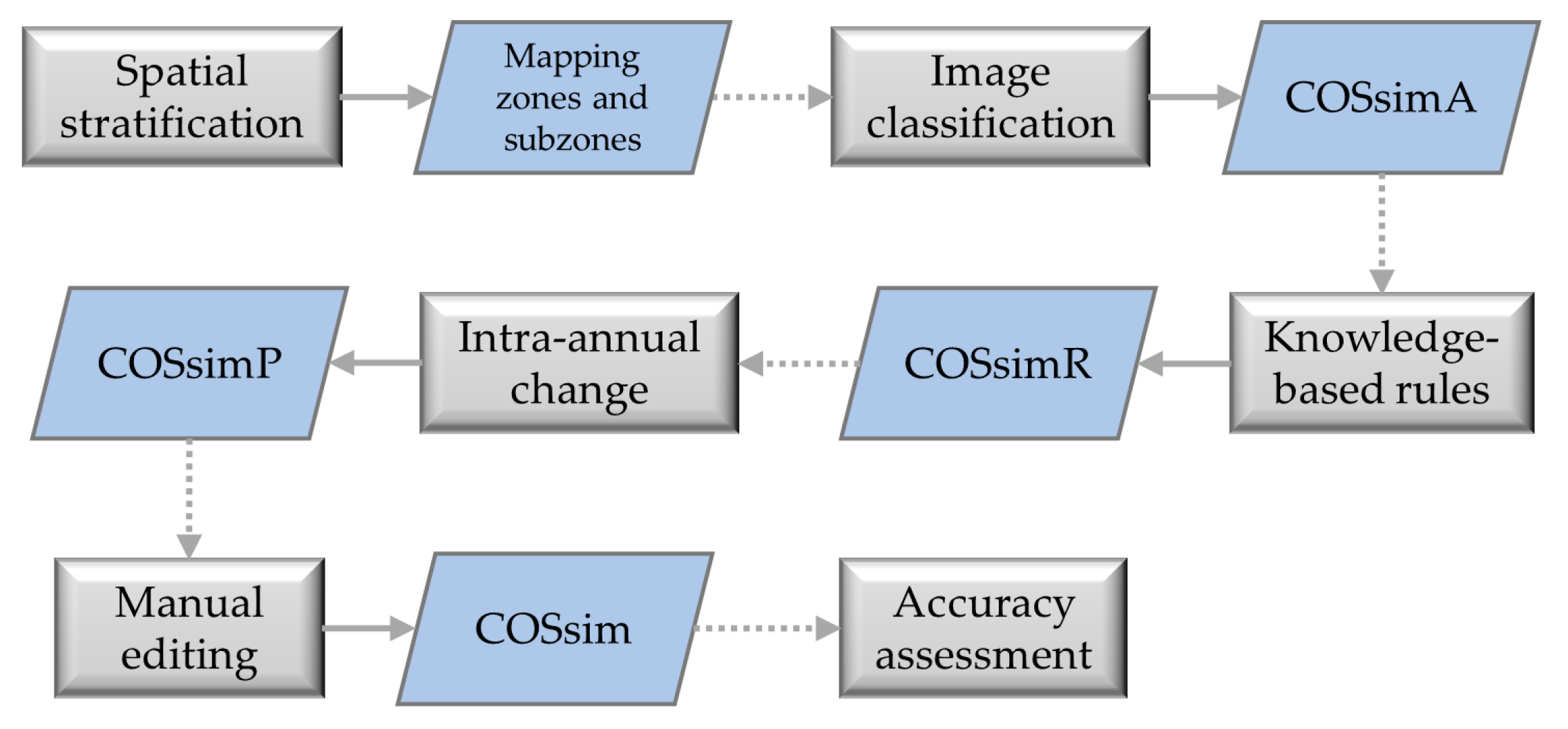
Figure 2 shows a general view of the methodology applied to the Portuguese mainland, which is summarised as follows:
Spatial stratification defined two hierarchical levels of spatial strata, hereafter called mapping zones and subzones. A total of 14 mapping zones were defined to deal with the landscape diversity of Portugal. The mapping zones included five subzones to deal with specific land dynamics.
Four stages were defined for data analysis and mapping. First, supervised classifications of Sentinel-2 data were performed. The map produced, hereafter called COSsimA, is analogous to the outcomes of traditional approaches that rely solely on image classification.
Knowledge on the Portuguese landscapes and their dynamics was used to fix misclassifications. This stage combined expert knowledge and auxiliary data in logic rules to produce an improved version of the map, COSsimR.
Next, a procedure was employed to detect and classify abrupt intra-annual changes in forest and shrubland (mostly fires and clear-cuts) that occurred during the 2018 agricultural year. Often, such changes went unnoticed through the previous stages because part or most of the spectral information of the Sentinel-2 times series represented land cover before change. However, the class resulting from a recent change was desired on the map. The output of this stage is called COSsimP.
Finally, the maps of all mapping zones were combined, and manual edition was allowed to refine local errors and seams between mapping zones, producing the final land cover map (COSsim).
A protocol was implemented to assess the accuracy of the final map, but also of preliminary maps of the various stages and strata.
4.2. Spatial Stratification
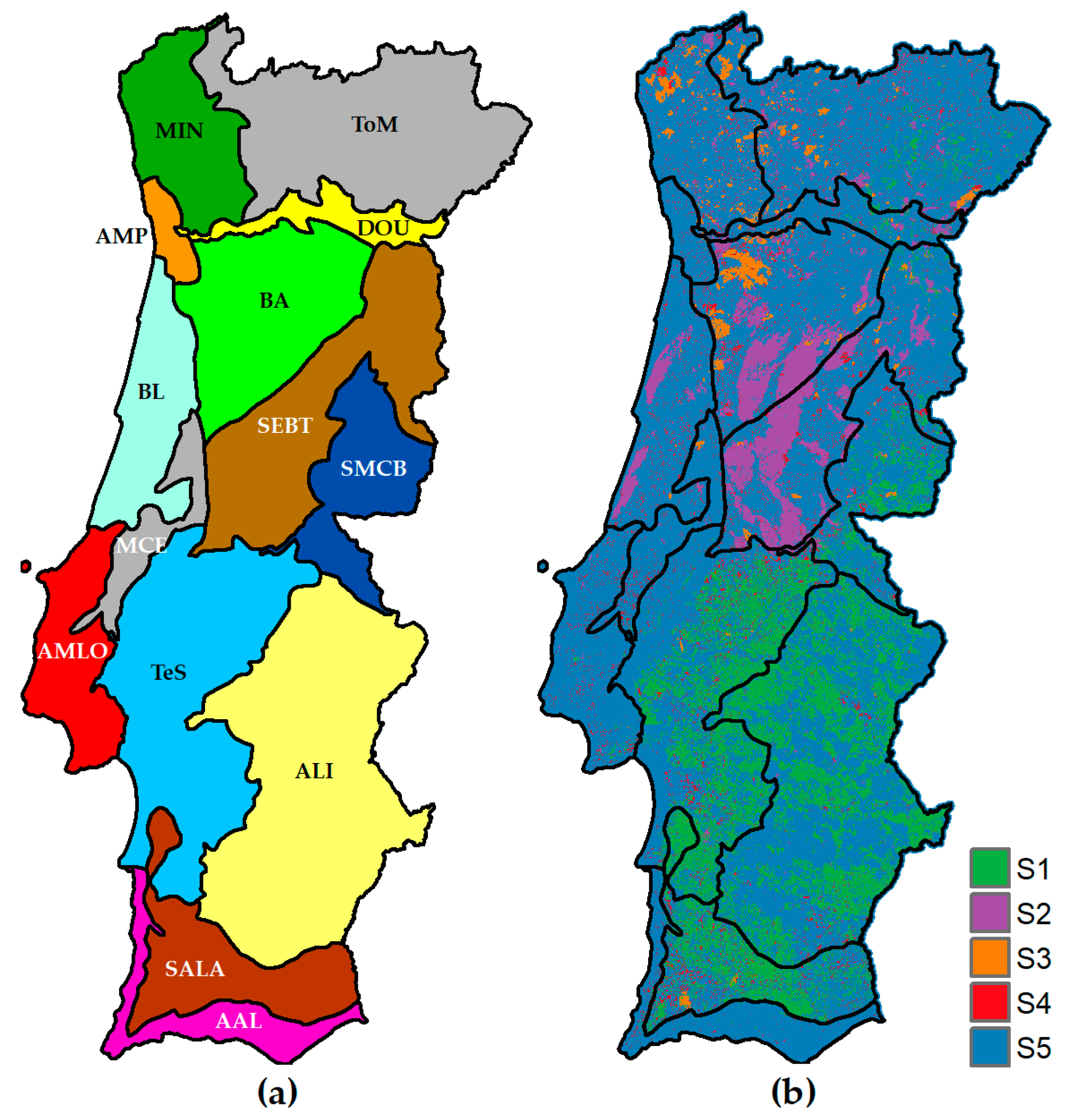
Mapping zones were defined following Cancela d’Abreu et al. [
43], who classified the Portuguese landscape in 128 landscape units based on a number of criteria, including land cover and land use. The original landscape units are very small in the context of image classification and thus were reinterpreted to suit a national image classification. The original landscape units were grouped into 14 larger units that divide the country into broad but distinct mapping zones (
Figure 3a).
The mapping zones were further divided into subzones (
Figure 3b) representing different characteristics and change dynamics of the territory. The subzones were used to implement specific procedures in map production while processing each mapping zone. Subzone 1 includes areas dominated by forest and agro-forestry systems of evergreen oaks known in Portugal as
montado. In
montado, tree density is highly variable in magnitude and spatial patterns, varying between rather dense wood stands, sparse, and isolated trees. Furthermore, a diversity of low vegetation grows underneath and between trees, including crops, pastures, and occasional patches of shrubs. The uniqueness of these areas poses problems in mapping that needed special treatment. Subzones 2 and 3 correspond to areas of forest and shrubland that burnt in 2017 and 2016, respectively, which imposed procedures to deal with vegetation recovery. Subzone 4 also relates to disturbance of forest and shrublands but caused by clear-cuts during the period 2015–2018. Subzone 5 is the remaining area, not included in previous subzones. For simplicity, the subzones are hereafter referred to as S1, S2, S3, S4, and S5.
4.3. Image Classification (COSsimA)
Image classification produced the first preliminary map, COSsimA, RF [
44] in R environment [
45] via the package randomForest [
46]. This map was obtained through the combination of two classifications. The first classification was general and included all classes (level 3) of the nomenclature defined (
Table 1). However, the classification suffered from large omission errors of evergreen oaks, making a large part of the country look treeless. These errors were particularly serious in South Portugal, where S1 subzones are large. In these subzones, the typical sparse and isolated distribution of oaks are largely associated with mixed pixels typically excluded from training samples, and classifiers have no means to learn that pattern. Furthermore, the diversity of low vegetation found underneath and between trees adds heterogeneity to the landscape, worsening classification errors. To address this problem, the second classification performed was dedicated to detecting tree crowns of evergreen oaks in S1 subzones. This classification used a more simplistic class nomenclature. The goal was to find the pixels that should be classified as evergreen oaks and superimpose them on the first classification. Details on both classifications are provided below.
4.3.1. General Classification
Sentinel-2 spectral data (i.e., composites, spectral indices, and metrics) and the DTM of Portugal were used as classification features. RF was trained separately in spatial strata, allowing classification to adapt to local conditions in two ways. First, the mapping zones were classified independently from each other and based on dedicated training data. Second, the classes effectively trained varied across subzones. That is, each subzone used a customised set of training data selected from those available for the mapping zone. This was possible because the training samples represented training classes instead of the final map classes. The purpose was to gain control over the spectral diversity of the map classes and use their various spectral traits differently. For example, training data representing regeneration of burnt shrublands could be collected for a given mapping zone but used only in subzones S2 or S3. This enabled the classifier to learn spectral patterns relevant for subzones where they mostly occur while avoiding commission errors to spread freely elsewhere.
Sample size varied as a function of the area of the mapping zones. Specifically, all training classes had the same number of training pixels in a given mapping zone, but this number varied across mapping zones, with a minimum of 1000 and a maximum of 6000 pixels per training class. The training pixels were selected randomly within limits of polygons, which were generated either automatically or manually (
Table 2) to represent the training classes. Polygons automatically generated resulted from the intersection of several auxiliary datasets (described in
Section 3.2), representing compatible land cover information [
47]. For example, polygons representing eucalyptus were shaped by intersecting the area of that class in COS and the area classified as broadleaves in DLT. The goal was to discard areas where different sources disagree on land cover classification to overcome inadequate characteristics of the datasets, such as large MMU. However, other issues remained. A typical case relates to the fact that COS is mostly a land use map and that can conflict with land cover (e.g., forest land temporarily without trees). Moreover, the 2015 versions of the HRL were used and could be outdated. Thus, additional filtering criteria such as a threshold of NDVI were needed to remove areas possibly mislabelled as forest or other vegetated cover.
Polygons manually generated were obtained through visual interpretation of the orthophoto maps and Sentinel-2 data. The decision of producing polygons manually to extract training pixels was made whenever the automatic procedure delivered poor results for classes that could impact considerably on the general quality of the map and there was no perspective of improvement in later stages. Problems in automatic training generation could have different causes. One common cause was error of the auxiliary datasets, resulting in mislabelled polygons. Since these errors commonly involved spectrally similar classes, mislabelling could enlarge classification errors. Shrublands were delimited manually to reduce confusion with forest. Furthermore, sometimes few and small polygons were generated automatically, thereby limiting the number of pixels available for training. Typical cases correspond to disagreements between broadleaves and conifers in different datasets. These situations forced manual delimiting for some tree species in a few mapping zones. Additionally, all polygons, either automatic or manual, were eroded with a negative buffer to avoid errors related to geometry and generalisation of the original sources.
4.3.2. Evergreen Oaks Classification
The second classification focused only on S1 subzones as the purpose was to detect tree crowns of evergreen oaks [
48]. Another set of training samples was collected to train the classification independently for each mapping zone. These samples represented classes expressing transition from treed to non-treed vegetation. The purpose was to perform gradient tree mapping [
49] by means of pure and mixed training pixels expressing gradual levels of abundance of four elements, namely oaks, shrubs, grass, and soil. However, each of the training pixels included only a maximum of two elements expressing gradient levels between oaks and one of the remaining three elements. The abundance of each element in the pixels was defined in four categories according to the order of abundance of oaks: 100%, 80%, 20%, and 0% of cover. A total of 12 classes were defined and approximately 50 pixels were manually collected per class in each mapping zone based on visual interpretation of the orthophoto maps and Sentinel-2 data. Spectral data of August 2018 were used to explore the spectral contrast between the evergreen oaks and the vegetation that dries during summer. The spectral bands of the monthly composite and the respective spectral indices were used as classification features in addition to the elevation extracted from the DTM of Portugal.
Due to the nature of the training samples, the classification output depicted a gradient of tree cover (100%, 80%, etc.). However, the goal was to identify the pixels which should be classified as evergreen oaks. As a general rule, all pixels with 20% or more crown cover were considered appropriate to represent evergreen oaks in COSsimA [
48]. All pixels considered as oak crowns were superimposed on the first classification. Thus, all pixels in S1 subzones were reclassified to evergreen oaks if classified as such in the second classification, thereby minimizing the initial omission error of the class. The pixels not classified as evergreen oaks maintained the class of the first and general classification.
4.4. Knowledge-Based Rules (COSsimR)
If-then-else rules that combined expert knowledge and auxiliary data were applied on COSsimA to produce COSsimR. The rationale was that disagreements between COSsimA and the auxiliary datasets could reveal problems in the former. Action was taken when the information mapped in the auxiliary datasets was more reliable, and pixels were relabelled to a more likely class set by the auxiliary dataset. The rules varied as a function of the mapping zones and subzones as related to different landscapes and dynamics. A general structure was defined to apply rules, which included three main blocks.
The first block used COS18 to relabel pixels that were very likely misclassified. For example, disagreements between some tree species in the map and COS18 were suspicious. Pixels linked to Maritime pine in COSsimA and Stone pine in COS18 were relabelled to the latter because confusion between conifers is common in satellite image classification, while COS benefits from reliable visual interpretation of orthophoto maps. All classes of the map were eligible to be reclassified in this block of rules.
The second block of rules used the HRL products. The various HRL used, which are dedicated to specific land cover types such as impervious surfaces in IMD, enabled some specific misclassifications to be relabelled. For example, commission errors of artificial land were somewhat abundant in some agricultural areas and relabelled to bare soil where no impervious surface was mapped in IMD. The HRL used were IMD, DLT, TCD, Grassland, and WAW.
The third and last block of rules used three different spectral–temporal NDVI metrics to distinguish between shrubland, natural grassland, and bare soil. The metrics used were the maximum and minimum annual NDVI, and the difference between the 25th and 75th quantiles. For example, a pixel labelled as bare soil and presenting high maximum NDVI could be relabelled as natural grassland, since bare soil should never reach a high annual NDVI value. These annual NDVI metrics were in some cases also used in the first and second blocks of rules as an additional condition to accept relabelling.
4.5. Intra-Annual Change (COSsimP)
Change detection was performed through the analysis of the NDVI time series. The method, based on [
50], calculated the variation of the NDVI within a moving time window for each instance of the time series. The variation was the difference between the NDVI after and before each instance considered. That is, the difference between the medians of the five instances after and before the central and moving instance. The largest decrease of NDVI along the time series was returned and assigned to the pixels. A threshold was then defined to identify pixels potentially associated with loss of vegetation. The threshold was set at −0.17 after visually analysing a set of random points drawn for this analysis. Change detection was applied only to pixels classified as forest trees or shrubland in COSsimR because they corresponded to potential cases of unnoticed intra-annual fires and clear-cuts that should be mapped. This was the only spatial constraint imposed to the analysis. That is, this stage did not follow the subzones, and the entire area of the mapping zones classified in COSsimR as forest trees or shrubland was analysed together.
The pixels flagged as associated with an abrupt decrease of NDVI were classified again. This time, only the composite of October 2018 was used for classification to ensure that all potential changes were captured even if occurring at the end of the period analysed. The training pixels used at the first stage to perform COSsimA were reused, but the training pixels with a large decrease of NDVI (below the threshold) were discarded. If-then-else rules were applied to introduce logic and realism to the changes and their classification. For example, pixels classified as forest trees in COSsimR could be reclassified as bare soil in COSsimP, or they could be reclassified as forest trees again. The latter happened when false changes were detected by the NDVI-based analysis. Changes between tree species from COSsimR to COSsimP were not allowed.
4.6. Manual Editing (Final Map)
All mapping zones were merged to produce the complete map of mainland Portugal. Final editing based on manual correction was implemented to remove persisting errors. Errors were found visually, and some guidance was provided by COS18. Although differences between the two maps are inevitable due to divergent mapping settings, suspicious differences covering a considerable area were revisited. Attention was also paid to the borders between the mapping zones. A few artefacts along the borders were found and mainly associated with classes prone to confusion, such as agriculture and natural grassland, resulting in the same patch, such as a crop field, being classified differently in the two sides of the border. When errors were found, polygons were manually delineated with two associated attributes, the wrong map class and the correct class. These polygons were used to relabel the wrong pixels.
4.7. Accuracy Assessment
A protocol to assess the accuracy of the maps was defined and included the three basic components of an accuracy assessment, namely sampling design, response design, and analysis [
51,
52]. The protocol was implemented in each mapping zone independently. Stratified random sampling collected the validation samples using the pixel as the sampling unit. COSsimA provided the sampling strata considering the nomenclature of 13 classes. The standard procedure was to collect 25 pixels per class.
The designed response was based on visual interpretation of the auxiliary datasets previously described (orthophoto maps, etc.) to decide on the reference class that each pixel represented on the ground. This procedure was performed considering a window of 3 × 3 pixels around the sampling units to provide context and minimise potential negative effects on classification caused by registration errors of Sentinel-2 images [
53,
54]. More than one reference class label per pixel was allowed to accommodate reference class ambiguity, for example when pixels were found in the transition zone between two land cover classes. Agreement was defined as a match between the map class and one of the reference labels [
52,
55].
Confusion matrices were produced with the validation samples to estimate the accuracy of the maps. The accuracy of the final map of Portugal was assessed based on a global confusion matrix produced from the combination of all validation samples.
All accuracy estimates calculated based on the confusion matrices faced the issue that the strata initially used to draw the validation samples were different from the maps assessed, hence violating the assumption of commonly used estimators that the sampling strata and the map assessed are the same. When it is not the case, the estimators of Stehman [
56] are recommended. These estimators calculate the proportion of area of each class in addition to the overall, user’s, and producer’s accuracies. Confidence intervals at the 95% confidence level are also calculated.
5. Results and Discussion
5.1. Map and Statistics
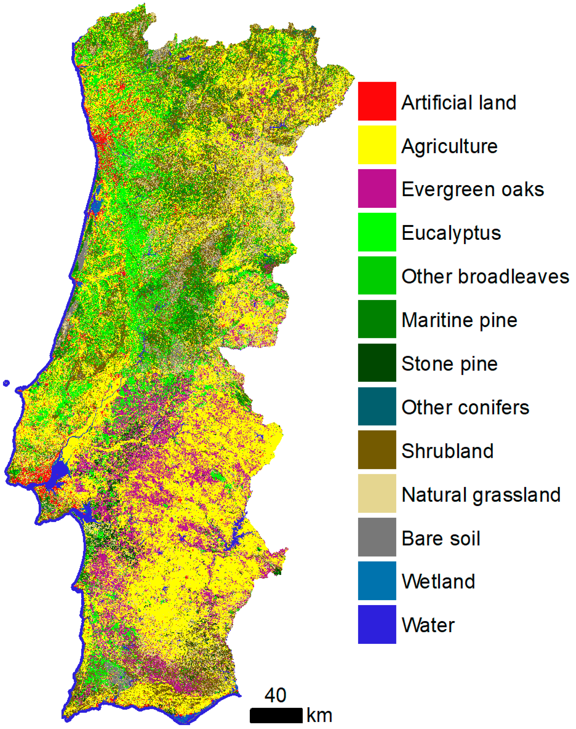
The land cover map produced for the reference year of 2018 is presented in
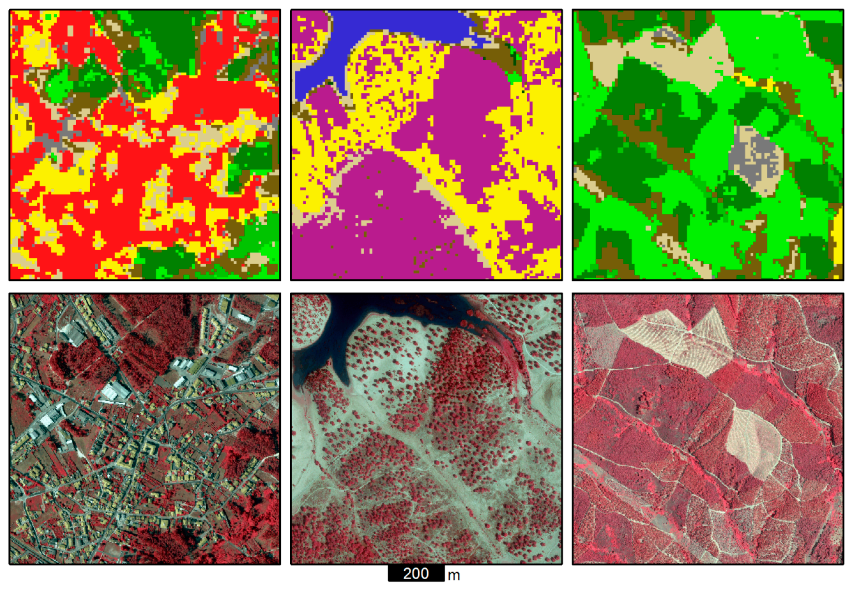
Figure 4. The main and general traits of the Portuguese land cover are apparent, such as the large forest area in the centre, evergreen oaks and agriculture mixed in agro-forestry systems in the south, and Lisbon and Porto metropolitan areas. A closer look at the map reveals the native spatial resolution of Sentinel-2 data, where different land cover classes intermingle (
Figure 5). In such cases, the map looks noisy, but at the same time it appears richer as small objects on the ground such as trees and buildings arise on the map. This provides a different view of the landscape when compared to traditional land cover maps of Portugal such as COS and CLC.
The global accuracy of the map is estimated at 81.3%, with a confidence interval of ±2.1%. The confusion matrix is presented in
Table 3. The classes mapped with higher accuracy are water, evergreen oaks, agriculture, and eucalyptus, all with accuracies > 86%, both the producer’s accuracy (PA) and user’s accuracy (UA). In some cases, accuracies are >90%, namely the PA of agriculture, evergreen oaks, and water. Water also exhibits >90% of UA. This means the omission and commission errors associated with these classes are relatively small and the observation of these classes on the ground is closely related to their appearance on the map. Other classes are mainly associated with one type of error, either omission or commission. For example, the omission error of wetlands is large (PA = 47%), but most of the wetlands mapped correspond to real observations on the ground (UA = 96%). Most problematic classes are other conifers and bare soil, with both accuracies < 67%.
Causes of misclassification can be numerous. Traditional spectral confusion between some classes is expected and indeed revealed in the confusion matrix, such as between shrubland and tree species, and artificial land and bare soil. A particularly large confusion is observed between natural grassland and agriculture because the former can be physically and seasonally similar to agricultural land, namely managed grassland and annual rainfed crops. Confusions can also be caused by factors other than obvious spectral similarity, such as the broad conceptual definitions of the classes. For example, natural grassland, in addition to being similar to agriculture, can accommodate a gradient of vegetation cover ranging from rather sparse vegetation to dense cover of tall herbaceous vegetation. The conceptual limits of the class are on the fringe of two other classes, bare soil and shrubland. Therefore, natural grassland is also confused with them.
For the less detailed thematic level 2, which aggregates the tree species in broadleaves and conifers (
Table 1), the overall accuracy is 82.6% (±2.1%). This represents an increase of 1.3% compared to the most detailed level 3. The increase is small because confusions among broadleaves and conifers represent a limited extent of the map. Considering the nomenclature of level 1 (6 classes), the overall accuracy rises to 89.7% (±1.8%), representing an increase of 8.4% as compared to level 3. In this case, as fewer classes are defined, more confusions are neutralised, for example between shrubland and natural grassland.
Users of the map should be aware of the misclassifications discussed above and the varying per-class accuracy. The value of the map may be larger for users interested in classes associated with larger accuracy, such as some tree species. For example, the map may be useful for applications related to wildfires as tree species represent different behaviour in fire spreading. On the other hand, users interested in wetlands may find the low PA of the class limiting.
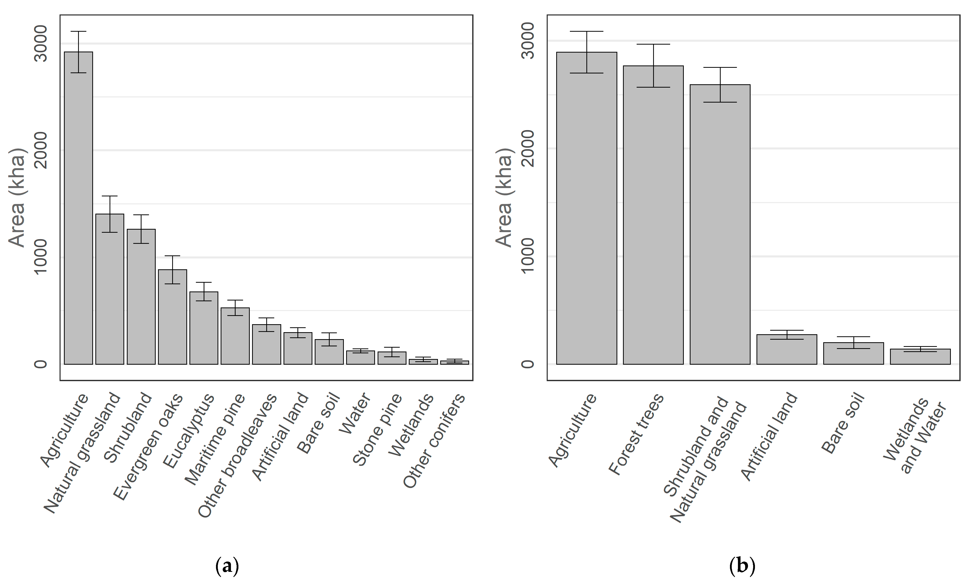
The accuracy assessment implemented provides estimates of the area occupied by the classes.
Figure 6 shows the area of each class and the respective 95% confidence intervals. The most abundant classes are agriculture, natural grassland, shrubland, and tree species. Estimates of area are also provided for the less detailed thematic level 1 to provide a more balanced view of the main land cover classes. Agriculture is followed by forest trees, and shrubland and natural grassland. Statistical uncertainty obscures which of these three classes occupies more area as their confidence intervals overlap.
These estimates provide new insights on land cover of mainland Portugal. For example, a large area of the country is occupied by shrubland and natural grassland. This may be surprising, especially for users familiar with other maps of Portugal, which traditionally show these vegetation types as less abundant. However, some issues should be noticed. First, it is expected that the spatial resolution is fine enough to capture small features of the landscape, such as forest clearings, often obscured in traditional maps such as COS and CLC due to their large MMU. Small MMU can favour the representation of classes associated with small patches. Additionally, COS and CLC include agro-forestry areas as a distinct class in their nomenclatures because of their MMU, but the new map with pixels of 10 m assigns the area occupied by agro-forestry areas to their constituents, such as forest trees and agriculture (
Figure 5). Then, maps such as COS enclose strong land use concepts in their class definitions and, for example, forestry areas temporarily without trees (e.g., due to clear-cuts) remain mapped as forest. In the new map, the situation is different and mapping momentaneous land cover is preferred, hence often showing shrubs, little, or no vegetation in forest patches cut or burnt. Indeed, the map represents the territory for the 2018 crop year starting from October 2017. Portugal suffered the tragic fires of June and October 2017, which together burned more than 500,000 ha in total (subzone S2 in
Figure 3b). The effects of those fires, and others from previous years, had a profound impact on forest and reduced the area occupied by trees. Fire scars are commonly mapped as shrubland, natural grassland, and bare soil. All these differences impact on the statistics potentially derived from the map. Therefore, caution must be taken while comparing the new map with other maps such as COS and CLC.
5.2. Spatial Stratification
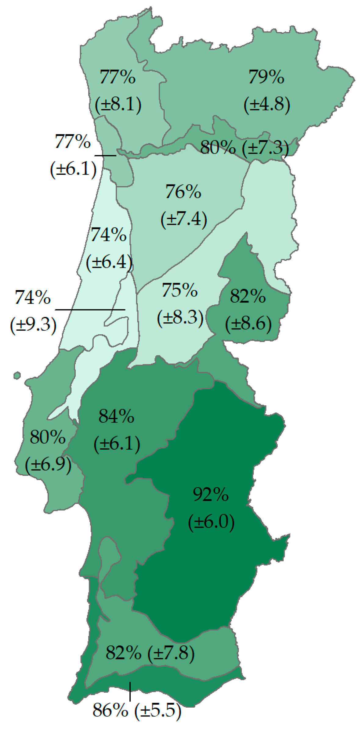
The definition of mapping zones and subzones allowed the implementation of tailored procedures, including customised training datasets and knowledge-based rules. The goal was to adapt mapping to local conditions and address specific problems. However, map accuracy is expected to vary across space in any case, and
Figure 7 shows the global accuracy achieved in each mapping zone. Larger accuracy values were attained in the south of Portugal, and the largest mapping zone, ALI, was mapped very accurately, with global accuracy possibly exceeding 90%. Mapping was less successful in other mapping zones in which the estimated global accuracy is <80%.
Possible causes for varying map accuracy may be related with the physical environment of Portugal. The mountainous topography and small land ownership of central and northern Portugal produce more fragmented landscapes, which complicates mapping. Additionally, larger precipitation and moderate temperatures may contribute to less evident seasonal variations for some types of vegetation, making analysis of Sentinel-2 time series less effective in some cases.
Other possible cause may be the occurrence and dynamics of land cover change events, such as fires. This relates to the subzones defined, and
Table 4 shows the global accuracy for the five subzones. Note that equivalent subzones from the different mapping zones were merged for this analysis because the validation samples are too small to assess the accuracy of each subzone alone. Even after merging, subzones S2, S3, and S4 all together represent a small proportion of the country (<11%), thus including few sampling units, which makes the confidence intervals of the estimates wide. However,
Table 4 shows that S2 subzones are associated with lower global accuracy, approximately 73%. These subzones, representing areas burnt in 2017 (i.e., shortly before the mapping reference year of 2018), encompass challenging cases for mapping due to varying scenarios of fire severity and potential vegetation recovery. S2 subzones, although relatively small for the size of the country (~5%), form an extremely large area if considered that it was burnt in a single year, and contributed for the modest results observed in central Portugal where they concentrate (
Figure 7), namely in mapping zones BL, SEBT, and SMCB.
Also associated with fires, but of 2016, S3 subzones present a global accuracy of ~83%. In these subzones, more time has elapsed since the vegetation burnt, and hence the trajectory of recovery was clearer. Clear-cuts since 2015 included in S4 subzones are a similar case, perhaps mapped with slight larger accuracy (83.4%).
The subzones occupying larger areas, S1 and S5, represent the most stable land cover in the country in recent years, but represent different cases. S5 subzones correspond to 73% of the country and were mapped with a global accuracy close to 80%, which largely contributes to the thematic accuracy of the final map (81.3%). These subzones were associated with no particular difficulty other than the heterogeneous landscape found in the country. Image classification and knowledge-based rules were implemented in S5 subzones with the broadest focus.
S1 subzones posed particular difficulties and required an additional image classification to map evergreen oaks (
Section 4.3.2). Preliminary tests revealed the effectiveness of the approach to mitigate omission errors, especially associated with low density and scattered distribution of trees [
48], resulting in the largest global accuracy of ~90%. A key aspect for the success of the classification was the spatial stratification based on COS18, which very accurately delimits the distribution of oak species, thereby avoiding confusion between tree species. As a result, the new land cover map presented here is the first map based on Sentinel-2 data that includes evergreen oaks as a distinct class.
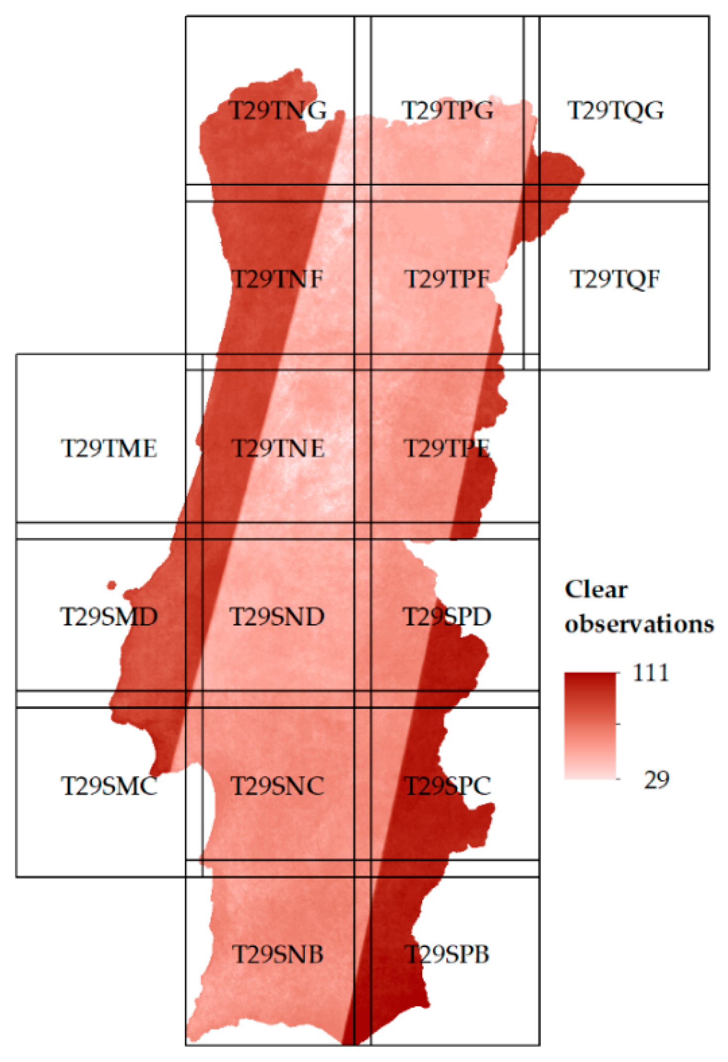
Beyond the spatial division of the territory related to the methodology, additional divisions were latent as a consequence of the Sentinel-2 data. They are divided in tiles and offer a large range of clear-sky observations provoked by the satellite orbits (
Figure 1). Therefore, artifacts could emerge between the borders of all these divisions. Manual editing of the map corrected a few border effects between mapping zones, but not between subzones, possibly because subzones share training data and are included in similar landscapes. Furthermore, no special attention was given to the borders along Sentinel-2 tiles and orbits as no artefacts were found to be particularly associated with them. This is possibly due to atmospheric correction [
27] and the use of median composites [
57]. The latter produced seamless classification features for all of the territory and attenuated all the differences in data availability that could impact on image classification and post-classification analysis.
5.3. Multi-Stage Approach
The land cover map of Portugal was produced through a series of stages, from which preliminary maps (COSsimA, R, and P) were produced along the way. Replicating the accuracy assessment (with the same validation samples) for COSsimA, resulting from image classification, reveals an overall accuracy of 70.2% (±2.3%). The difference between COSsimA and the final map is 13.3%, confirming the added value of our stepwise approach to improve the quality of the map. Several reasons can explain the errors in COSsimA, and one possibility is the quality of training. Manual training was used to tackle main problematic classes, but some classes mapped with low accuracy remained automatically trained. Varying quality of automatic training data is expected as procedures for their generation varied, depending on auxiliary datasets with different characteristics, including thematic detail, per-class accuracy, and date. For example, HRL of 2015 were used, which can show disagreements between 2018 due to recent land cover change. Disagreements between the auxiliary datasets resulted in excluding a few areas from the automatic training, potentially impacting on classification. Alternative generation of training data can be considered to improve their quality, such as refining the filtering criteria used and adding more auxiliary data [
58]. Other reasons limiting classification accuracy may include the length of the time series (one year), classification features, classification method, and so forth.
In any case, previous work suggests an inherent difficulty to classify land cover in south Europe [
9,
19,
20]. These examples correspond to global and continental land cover maps based on classification analysis not developed in detail for specific countries. Therefore, the accuracy of the maps is mainly subject to the ability of the supervised classification and main analysis employed to achieve the final thematic accuracy. However, when classification accuracy is modest, additional analysis gains relevance in inferring land cover. Therefore, COSsimA was subsequently improved throughout post-classification stages.
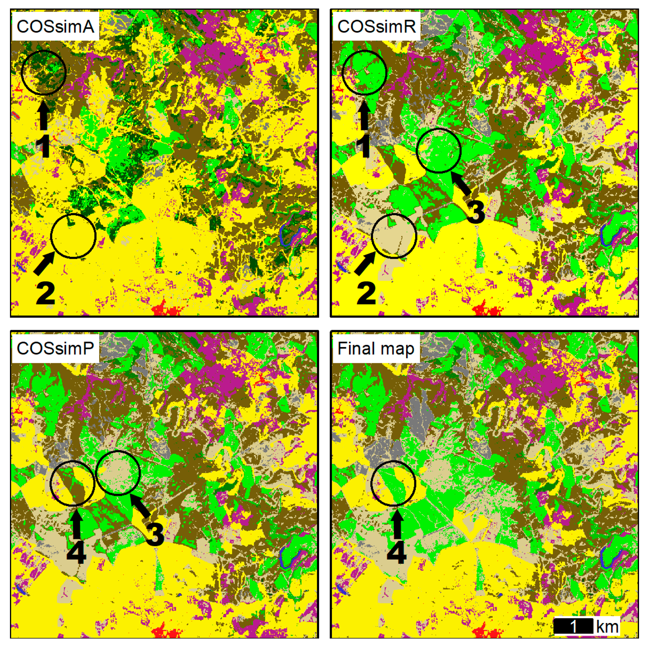
Figure 8 shows an area of particular complexity, where a number of improvements were introduced during map production. Zones 1 and 2 (flagged with circles in
Figure 8) point to areas improved by knowledge-based rules. In zone 1, there was confusion between shrubland, conifers, and broadleaves, and zone 2 highlights natural grassland previously misclassified as agriculture. Knowledge-based rules were the main responsible stage for improving the map, and alone modified 28.7% of the pixels to produce COSsimR, and the overall accuracy increased by approximately 13.3%. That is, COSsimR already presents the estimated overall accuracy of the final map.
The subsequent stages together (intra-annual change and manual editing) modified only 0.5% of the area as they focused on localised refinements. Therefore, these stages had no impact in terms of thematic accuracy estimates. However, the refinements can be noticed. For example, zone 3 in
Figure 8 was detected as corresponding to a clear-cut of eucalyptus. Since the clear-cut was observed at the end of the time series (August and September 2018), most of the spectral information was associated with eucalyptus and thus classified as such, until COSsimP reveals its removal. As another example, zone 4 was misclassified as natural grassland and shrub throughout the mapping stages of analysis, and finally identified manually as eucalyptus. The difficulty of identifying this patch of eucalyptus is explained by low tree density.
The two first stages, image classification and knowledge-based rules, were the most important. The link between the two stages is strong because knowledge-based rules are shaped according to the problems received from the precedent stage. While this was designed to face the insufficient quality provided by a more traditional image classification and allowed the quality of the map to largely increase, there are some downsides. For example, defining rules can be time-consuming and too dependent on auxiliary data. However, alternative ways of implementing the multi-stage approach can attenuate these issues. For example, defining rules can move towards probabilistic or modelling approaches [
59].
Adding mapping stages of analysis is a choice allowed by the methodology and it offers new opportunities to improve mapping. For example, including intra-annual change, such as clear-cuts observed very close to the end of the time series, was more of a desire than a necessity. It would also be acceptable to map land cover before change as associated with most of the year analysed. However, mapping recent changes in forest and shrublands ensured that the status of vegetation represents a specific and known timestamp (end of the time series), which makes it clearer to the end-user what the map represents. The methodology is flexible to accommodate additional stages as needed and desired to tackle specific problems or divide complex mapping tasks in several parts.


 ,
, 
