Article

Manifestation of Spiral Structures under the Action of Upper Ocean Currents

1
Institute of Applied Physics of the Russian Academy of Sciences, 46 Uljanova St., 603950 Nizhny Novgorod, Russia
2
Faculty of Informatics, Mathematics and Computer Science, National Research University Higher School of Economics, 25/12 Bolshaya Pecherskaya Ulitsa, 603155 Nizhny Novgorod, Russia
*
Author to whom correspondence should be addressed.
Remote Sens. 2022, 14(8), 1871; https://doi.org/10.3390/rs14081871
Submission received: 9 March 2022 / Revised: 6 April 2022 / Accepted: 12 April 2022 / Published: 13 April 2022
(This article belongs to the Special Issue Remote Sensing of the Sea Surface and the Upper Ocean)

Abstract

:
The traditional approach to the interpretation of spirals observed in radar, optical and radiometric panoramas of a sea surface is based on equating the outer spiral scale with the scale of a manifesting eddy, but the validity of this approach has been poorly studied. Using the maximum cross-correlation (MCC) method for multispectral satellite images containing a spiral structure, we found a significant discrepancy between the structures of horizontal velocity fields and the geometrical characteristics of spiral structures in each band. Each velocity field demonstrated a pair of points of zero velocity with a km-scale difference between their positions in different bands. In order to describe the observed features, an analytical description of the upper-ocean current composed of a spiral eddy and of a homogeneous drift (related, in particular, to wind forcing) is proposed. This simple model states that the spiral characteristics and the position of the spiral center depend on a drift current even when the genuine characteristics of the marine eddy are fixed. The studied example shows that the diameter of an eddy core may significantly (2–3 times) differ from the outer scale of the spiral, which demonstrates the incorrectness of the traditional approach of spiral structures interpretation.

Graphical Abstract

1. Introduction

The ability of inhomogeneous currents, in particular, vortex currents, to redistribute suspended matter, ice floes, surfactants and heated water masses leads to the manifestation of marine eddies in radar, optical and radiometric high-resolution panoramas of a sea surface [1,2]. Recent investigations revealed an important role of marine eddies in aspects of ocean global mixing [3], local mixing affecting biological processes, phyto- and zooplankton distribution [4,5,6], global heat and flux exchange [7,8], vertical mixing of the ocean [9,10], estimation of shelf anthropogenic load [11,12], etc.
The traditional approach to the interpretation of these spiral structures in satellite images of the ocean upper layer is based on direct equating the outer spiral scale with the scale of an eddy. For example, in [13,14,15,16] the analysis of eddies’ characteristics in a fixed region (rotation directions, distribution of eddies’ sizes, ratios of the lengths of eddies’ axes) is based on the interpretation of heterogeneously distributed surfactant films or ice floes forming spiral structures in radar panoramas of a sea surface. In this case, the eddy diameter is determined as the mean length of the two quasi-perpendicular sections across the spiral center, ending at the most distant spiraling line [16]. Moreover, the eddy rotation direction is determined in correspondence to the direction of the spiral swirl with the assumption of its convergence [17,18,19]. This approach is extended to the interpretation of spiral structures manifestation in different ranges of the electromagnetic spectrum and appears to be the prevailing method, if not the only one, in the literature. Despite a widespread application of this approach, the relation between a field of currents in the upper ocean layer and the geometrical characteristics of manifesting spirals is poorly studied. The remarkable facts are that the variation of the observed spirals’ diameters may achieve the order of magnitude [14,15] and that altimetry data statistics may demonstrate significantly distinct distribution of eddies’ sizes in a fixed water area (for example, [16]).
Remote sensing methods are applied to retrieve the upper-layer currents along a large water area without conducting in situ measurements. The application of onshore HF radars provides the characteristics of the current field of the upper layer, about 0.5 m thick, which is strongly affected by wind [20]. It should also be noted that the eddies reaching the shelf are already being affected by the seabed topography. The most common method of measuring marine currents with scales of tens and hundreds of km is satellite altimetry [17,18,21], which is characterized by the high accuracy of the obtained dynamic topography (up to 1–2 cm, according to [19]). The velocities of subsurface jet-like flows, oceanic fronts and mesoscale eddies are retrieved on the grounds of geostrophic approximation [22]. The accuracy of marine currents determination may achieve the order of cm/s on the scales of tens of km [23,24], but the efficiency of altimetry methods is geographically limited, since the geostrophic assumption is invalid in the equatorial band [25]. The retrieval of the characteristics of mesoscale eddies at polar latitudes is even less available, since the Rossby radii can be comparable or less than the resolution of the modern altimetry data [26,27,28].
Another way of retrieving upper ocean currents is based on matching sequential satellite (or aircraft-based) optical or radar sea panoramas. The analyses of shift of brightness irregularities between the frames provides the horizontal velocity field of upper ocean currents. In the literature, the most applied methods for such analyses are the Maximum Cross-Correlation method (MCC) (see [29,30,31,32,33,34,35,36] and the mentioned references) and the optical flow method [37,38,39,40]. The retrieval of currents using these methods may be performed through the analyses of ice drift [33], brightness temperature or its horizontal gradient distribution [29,30,37,41], visible upper layer irregularities such as surfactant slicks in the radar images [42,43,44], or phytoplankton patterns [39,45].
The MCC algorithm is a block-matching method that determines the similarity between two sequential image pairs based on cross-correlation coefficients. Justified by the apparatus of functional analysis, the optical flow method initially stemmed from the computer vision field. Each pixel of the image is characterized by brightness or color, being unalterable in sequential images. The velocity of each element is determined by the local displacement of each pixel considering that the velocities of nearby pixels are similar. The optical flow method is considered to be more reliable and to give higher spatial resolution than the MCC technique [40], especially for displacements of the order of 1 pixel or less. However, for greater shifts of elements between the frames, the two methods are in good agreement [46,47,48]. The preliminary estimation of an element’s displacements in the further discussed case allowed us to conclude that the MCC method characterized by easier calculations is appropriate for the processing.
The correctness of the horizontal velocity field retrieval using the MCC method is determined by the time interval between the consecutive observations of the studied area by satellites or airborne equipment [49,50]; in recent decades, the attainable time delay was significantly reduced from several hours [29] to the order of minutes [43].
This paper is devoted to the investigation of the relation between the horizontal structure of upper-ocean eddy currents and their tendency of form spirals, as well as to the development of an elementary analytical model describing these currents. The novelty of this investigation is the use of the MCC method for different bands of multispectral satellite images. Fine velocity fields, describing the inner structure of eddy-related currents, demonstrate the new peculiarities, and their analytical description is elaborated. The application of the obtained results to the retrieval of the genuine characteristics of marine eddies is discussed.

2. Materials and Methods

In order to obtain the characteristics of the velocity fields associated with marine eddies, the search of sequential high-resolution images of a sea surface with small time delay, low cloud coverage (<10%) and manifestation of spiral structures was performed. Overlapping of multispectral images from the satellites Landsat-8 OLI and Sentinel 2A MSI taken at small time intervals appeared to regularly occurr over the Baltic Sea; in particular, such a configuration was found on 25 July 2018 for the Gotland Basin (Figure 1), with the time of imaging being 9:47:50UTC and 10:04:30UTC respectively. For the bands used in the study, the spatial resolution of Sentinel 2A Multispectral Instrument (MSI) imaging was 10 m, and that of Landsat-8 Operational Land Imager (OLI) was 30 m; in order to process the images with the MCC method, the Sentinel image was resampled to the 30 m resolution by evaluating the mean brightness of groups of pixels.
The archived data of wind velocity in the observed region [51] demonstrated that a few days before the snapshots were taken, the wind velocity was stable, of about 1–2 m/s, and 6 h before it increased up to 3–4 m/s, had a north-east direction (the wind direction is shown in Figure 2) and remained stable during the observational period.
The Baltic Sea is characterized by fragmentation into separate basins with significantly different depths, salinity values, heating regimes and regimes of water exchange with the surrounding basins. In the summer months, the optical images of the Baltic Sea show heterogeneously distributed areas with increased turbidity and phytoplankton concentration [52].
The MCC technique was utilized to retrieve the horizontal current velocity field. Spiral bands observed due to increased phytoplankton concentration were used as features whose displacements were estimated in subsequent satellite optical images with dimensions of 26 × 45 km. To implement the MCC method, sub-images with sizes of 64 × 64 pixels2 (1920 × 1920 m2) were extracted from the initial images so that the centers of neighboring sub-images were displaced by 32 pixels in both directions (E–W, S–N). This 50% overlapping was performed to obtain additional information about the displacements at the boundaries and angles of each sub-image. The size of the sub-images and the overlapping coefficient determined the spatial resolution of the retrieved current velocity field. The velocity of each element was determined by finding the location of the maximum in the cross-correlation matrix obtained by comparing the subsequent sub-images (see [53]). The images used for the processing are shown in Figure 2 (images of Sentinel 2A MSI). An ensemble of Landsat-8 OLI images is not shown, since the difference between each pair of consequent images was not visually pronounced.
The size of a mesh element was determined to meet the requirements of the investigation of small-scale processes and of the presence of unique irregularities in each element. Note that the algorithm was focused on the determination of the maximum cross-correlation in the limited area, so that the maximum displacement corresponded to the element size. Considering the maximum horizontal velocity of 50 cm/s and the time delay of approximately 17 min, we estimated a maximum displacement (corresponding to the minimum element size) of about 500 m. Generally, the MCC technique has limitations for the correct velocity field retrieval associated with the displacement of a smooth band along itself [44], but the described spiral bands in Figure 2 are characterized by torn borders with a plenty of small-scale features (compared to the size of the mesh element), which allowed us to consider this error to be insignificant. It can be observed in Figure 2 that the concentration of irregularities significantly varies between the images of different bands and locally in each image. In order to minimize possible errors and to provide a smooth velocity field along the whole frame, the element size was finally chosen to be of the order of 2 km.
An example of the cross-correlation function typical for a 1D displacement is shown in Figure 3. Predominantly, the high amount of brightness irregularities ensured the substantially pronounced maximum of the cross-correlation function. The velocity in the mesh element was considered to be determined if the cross-correlation coefficient exceeded 0.5. In order to obtain more “specific” velocity values during the processing, a 3-point Gaussian subpixel estimation in the vicinity of a maximum value was performed for both directions of the displacement. Since the spatial discretization of the cross-correlation function is equal to the pixel size, the final velocity error related to the pixel size can be expressed as d V p s = 0 . 5 pixel size / time delay = 1.5 cm / s [54]. The absolute geolocation error occurring due to the displacement of the land position in images obtained by different sensors [42] was 0.7 cm/s for the west-east velocity component (here and after denoted as Vx) and 0.3 cm/s for the south-north component (Vy). This geolocation error was a systematic one, directed to north-east and remained the same in all bands.
In this study, the brightness irregularities present in the images were considered as passive markers, and the error associated with a possible active motion of phytoplankton was considered to be negligible, since this motion is mostly vertical and is characterized by velocities of the order of 10−3–10−2 cm/s [55].
The obtained horizontal velocity field for the green band is shown in Figure 4a. The first feature observed in the obtained velocity field is the presence of a pair of zero-velocity points: the first appears as a stable focus attracting spiraling streamlines in its vicinity, the second one resembles a saddle, attracting streamlines along one direction and repelling them along another. The velocity fields in the different bands demonstrated a qualitatively similar behavior.
Generally, the correctness of the application of the MCC method to velocity field retrieval is limited by the scale of the vertical displacement of water elements, which takes place between consecutive snapshots. If this displacement is small, one can observe the same water pattern in both images. To characterize the values of the vertical velocities, a divergence map is shown in Figure 4b for the green band. The divergence at each point with coordinates (i, j) was determined as follows:
d i v V 2 D ( i , j ) = V x ( i + 1 , j ) V x ( i 1 , j ) 2 d x + V y ( i , j + 1 ) V y ( i , j 1 ) 2 d y
where dx = dy = 960 m was a mesh step. The variation of the divergence maps in different bands was insufficient. According to the maximal value of divergence of 6 × 10⁻⁵ 1/s and the assumption of zero vertical velocity at the surface, the vertical displacement can be estimated as Δ z = V z Δ t 6 × 10 5 s 1 z × 1000   s 6 × 10 2 z , where Δt is the time interval between the images, z is the depth of the lower layer boundary. The small order of the out-of-plane displacement was sufficient to conclude that the application of the MCC method was correct in the described case ([56] and references herein). Another argument in favor of this conclusion is based on the high values of the cross-correlation coefficients: 0.83 ± 0.03 in the blue, green and red bands, decreasing to 0.65 in the NIR band.
These considerations are compliant with the typical time scales of processes affecting the sea surface state in the observed region. The timespan of submesoscale eddies is of the order of several weeks (for example, [57]), and the timescales of the upward supply of matter to the surface by submesoscale eddies is of the order of days [58]. The time scale of wind-induced upper ocean current modification is at least of the order of several hours [59]. No evidence of internal waves is present in the images; the appearance of ship wakes is insignificant on the observed scale. In this case, a sharp change of the surface conditions in 17 min is hardly possible.
In Figure 4a, a visual difference between the orientation of the spiral structure fragment and the velocity direction at each point is observed, especially in the western part of the image. The map of the vertical component of relative vorticity (Figure 4c) characterizing the vortex motion in the horizontal plane was determined at each point with coordinates (i, j) according to
r o t V 2 D ( i , j ) = V y ( i , j + 1 ) V y ( i , j 1 ) 2 d x V x ( i + 1 , j ) V x ( i 1 , j ) 2 d y
It showed that the focus-like point was significantly displaced from the center of the maximum vorticity area. In order to describe the observed features of the velocity fields and to explain this discrepancy, a simple analytical description is proposed.

3. Analytical Description

Let us describe analytically the structure of a velocity field composed of an axisymmetric eddy and of a homogeneous drift component [60]. The horizontal streamline is described in a polar coordinate system (r; θ) whose pole is collocated in an eddy center; the eddy tangential component is denoted as Vθ, the radial component directed outward the center is Vr. The streamline equation considering a homogeneous drift component with modulus W and direction Ψ can be expressed as [61]:
d r V r + W cos ψ θ = r d θ V θ + W sin ψ θ = d t
where W cos ψ θ is the projection of the drift component on the radial direction, and W sin ψ θ is on the tangential direction. The equilibrium points of the system of differential equations obtained from (3) are the points of zero velocity. Their coordinates (r*, θ*) are expressed as
V r 2 ( r * ) + V θ 2 ( r * ) = W 2 tan ( ψ θ * ) = V θ ( r * ) V r ( r * )
Referring to the literature regarding field measurements of currents inside marine eddies [62,63,64] and commonly used models for their description [65,66,67], it can be concluded that for an individual eddy, the function V ( r ) = V r 2 ( r ) + V θ 2 ( r ) demonstrates a gradual growth near the center, achieving the maximum value at distance R (which is commonly denoted as an eddy core) and then decreasing as the distance from the center increases.
The system (4) provides the conditions for specifying the positions of points where the velocity related to the vortex motion is balanced with the vector of a drift current. Depending on the relation between Vmax = V(R) and the drift velocity, the first equation of (4) may have 0 to 2 roots (Figure 5).
Let us now define the qualitative behavior of the streamlines in the case of two existing roots (W < Vmax). The eigenvalues of the matrix of the linearized system (4) in the vicinity of the equilibrium points are determined by the equation
λ 2 λ V r ( r * ) r * + V r r r * + V r ( r * ) r * V r r r * + V θ ( r * ) r * V θ r r * = 0
Thus, the character of the equilibrium point ( r * , θ * ) is determined by the coefficients:
b = V r ( r * ) r * + V r r r *   and   c = V r ( r * ) r * V r r r * + V θ ( r * ) r * V θ r r * = 1 2 r * ( V 2 ) r r *
In the polar coordinate system for the case of an axisymmetric eddy, −b coincides with the horizontal velocity field divergence, which is preserved when a homogeneous drift component is added:
b = V r *
The first equilibrium point, located on the increasing interval of the function V(r), gives c > 0. Further analysis reveals the following cases:
( a )   b 2 > 4 c ,   or   V r ( r * ) r * V r r r * 1 > 2 V θ ( r * ) r * V θ r r * 1 the   point   is   a   node .
( b )   b 2 < 4 c ,   or   V r ( r * ) r * V r r r * 1 < 2 V θ ( r * ) r * V θ r r * 1 the   point   is   a   focus .
The stability of the first point is determined by the sign of the horizontal velocity field divergence in the vicinity of this point. Real eddies, as field experiments [63,68] demonstrate, are characterized by a complex behavior of the radial velocity component. So, in some cases, with an integrally divergent eddy, the first equilibrium point may be stable, which corresponds to the converging spiral. Moreover, for a stationary current field, this point is observed in satellite images as a spiral center. In the case of a small radial velocity, according to the second equation of (4), the first equilibrium point is shifted in the direction close to crosswind and, according to Figure 5, this shift can achieve values of the order of R.
The second equilibrium point is characterized by the decreasing interval of V(r), which leads to c < 0. In this case, the eigenvalues of (5) are real and of opposite signs, thus the point is a saddle. An increase of a drift component leads to the merging of points (W = Vmax) into a saddle node and its further disappearance.
Figure 6 qualitatively demonstrates the difference between the initial velocity field of a marine eddy and the field consisting of an eddy and an additional homogeneous current. The equilibrium points are depicted as red and green dots (a focus and a saddle, respectively). In the first case, a saddle is infinitely distant from the eddy core (see, Figure 5 with W = 0), but an increase of the drift current absolute value leads to the approaching of the saddle point to the focus point. In the case of a relatively small homogeneous current, the presence of the saddle point constrains the “capturing properties” of the convergent eddy, i.e., limits the area of streamlines involved in the formation of spiral structures.

4. Discussion

The described analytical approach based on a simple model provides some important conclusions regarding the horizontal dynamics of the upper layer which is affected by marine eddies and homogeneous (on the scale of eddy) horizontal drift currents:
(1)
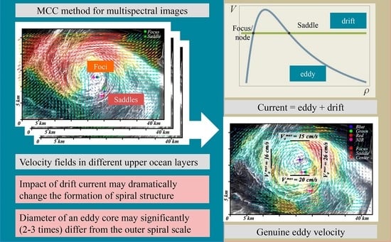
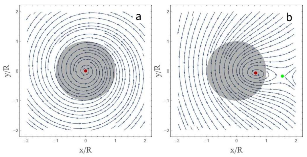
the geometry of the resulting current streamlines qualitatively differs from the genuine structure of marine eddies;
(2)
the velocity field may demonstrate the presence of a second equilibrium point, i.e., the saddle;
(3)
the position of the focus/node (which corresponds to the spiral center) depends on the drift current and may be significantly shifted from the eddy center—up to the scale of the eddy core.
The features that were predicted by this simple approach, such as the presence of a pair of equilibrium points (a focus/node and a saddle) in the structure of subsurface currents, were observed in the velocity fields obtained using the MCC method (green band—Figure 4a). The four obtained velocity fields demonstrated a qualitatively similar behavior, but the detailed analysis revealed that the positions of the zero-velocity points varied in different bands. Figure 7 demonstrates their positions in the region shown by a black square in Figure 4a. The character distances between the foci in different bands were the following: NIR/red—150 m, green/blue—390 m, green/NIR—1380 m. The exact positions of the points with zero velocity, shown in Figure 7, were determined automatically based on a linear interpolation of the velocity field in the vicinity of their approximate position. It should also be noted that, since the positions of the points of zero velocity were determined based on the velocity field, the velocity error determined the spatial error of these points’ positions. The region with the possible presence of a zero-velocity point is defined as the region where the velocity does not exceed the error values. As far as the geolocation error in different bands remains the same, the relative positions error is determined only by the stochastic error (dVps = 1.5 cm/s).
When indicating the distinction between the positions of the points of zero velocity in different bands, we should also estimate how the geometrical features of satellite imaging may affect the observation of a point with fixed horizontal coordinates but located at different depths. According to Figure 1, Sentinel 2A MSI observed the studied fragment in almost nadir direction—in this case, the geometrical optical error was negligible; the Landsat-8 OLI altitude was 705 km, the incidence angle of its observation in the studied area was about 7°. The obtained geometrical optical error was approximately one-third of the layer depth, which was of the order of meters. It can be concluded that the obtained discrepancy between the positions of the points of zero velocity in different bands exceeded all possible errors.
A result of the analytical description is that the positions of equilibrium points related to the given marine eddy depended on the additional drift current. The mean velocities over the entire studied area in all bands are shown in Table 1. An additional analysis revealed that these mean velocities can characterize a homogeneous large-scale current in the study area. With a constant mesh step, the averaging region was expanded by adding 5-, 10-, 15-, 20-, 25-km-thick frames at each side of the studied area. The analysis revealed that the variations of the mean velocity values did not exceed 5% of the initial values in the cases of 5–20-km-thick frames and increased up to 10–15% for a further expansion.
According to the analytical description, the genuine velocity field of a marine eddy can be retrieved by subtracting the homogeneous components. The horizontal velocity fields obtained after the subtraction of the mean velocities and the positions of the zero-velocity points are shown in Figure 8, which demonstrates a single center for all bands—the distance between corresponding points does not exceed 200 m, which is an order less than the mesh step and the spatial error of point position.
Let us discuss now why the original velocity fields observed in different bands may be distinct. It is known that ocean eddies are characterized by a three-dimensional structure which leads to a vertical water redistribution resulting in irregularities in temperature, salinity [69,70] and phytoplankton concentration [71,72]. The attenuation of light in water significantly depends on the radiation wavelength. Since phytoplankton is distributed vertically in the upper layer [73], using sea panoramas at different optical bands, we may retrieve horizontal velocity fields in layers of different thicknesses. Table 1 describes the bands that were used for the MCC processing. For the Baltic Sea waters, significantly affected by seasonal eutrophication, variations of the downward attenuation coefficients, introduced to characterize the spectral characteristics of the downward irradiance, are well studied for wavelengths in the optical range [74,75,76]. The depths of the observed layers can be estimated using the inverse attenuation coefficients from [74] with the assumption of a vertically uniform distribution of phytoplankton in the mixed upper layer. The estimated depths vary from the order of centimeters (NIR) to 3–4 m (Green band); the different channels present different but overlapping layers.
Since these bands correspond to layers of different thicknesses, we may assume that the variations of the mean velocities occurred due to the depth-dependent upper ocean current. There is a source of current depth dependency associated with wind forcing. The simple estimation of the wind-induced surface current as 3% of the moderate wind velocity gives approximately 10 cm/s, which is lower than the obtained values of mean horizontal velocities described in Table 1, which implies the additional effect of a large-scale current of another origin.
The typical time spans and vertical structure of a sub mesoscale vortex motion in the ocean may significantly differ from the corresponding characteristics of a homogeneous current, especially a wind-induced one. This may lead to the observed effect of the discrepancy between the geometrical characteristics of spiral arms and the original velocity fields. We assumed that in the described case, the spiral was formed in the conditions of a weak drift current which significantly increased several hours before satellite imaging, according to the previously described wind data. According to the typical scales and velocities, the time of spiral formation could be estimated as 40–60 h, and the sharp wind change was not able to promptly redistribute phytoplankton in compliance with the new velocity field [77]. It can also be interpreted as the effect of the memory of the spiral structure formation. The geometry of the retrieved genuine eddy current closely matched the geometrical features of a spiral structure.
In general, it is possible that the spiral formation proceeds in the presence of a strong drift current. Thus, despite the presence of a marine eddy, this drift may prevent the spiral formation or may restrain the scale of the spiral structure due to the appearance of a saddle point. This effect may cause a significant misinterpretation of the quantity and scales of eddies, even in the presence of many irregularities such as surfactants, ice floes or phytoplankton in the upper layer. Further investigation of similar cases of retrieved velocity components and the search for the patterns of the spiral structure is a perspective problem whose solution would be applicable for the development of accurate satellite data interpretation methods.
Finally, Figure 8 demonstrates the scale of an eddy core defined as the area of increased vorticity and maximal tangential velocities of eddy motion in each transect. It can be seen that the diameter of the eddy core was 2–3 times smaller than the outer scale of the spiral; this case clearly illustrates the incorrectness of a common approach based on direct equating the spiral scale with the eddy scale. On the contrary, the described technique, based on the MCC method and its interpretation, enable to separate the eddy velocity components and to estimate their genuine characteristics with high accuracy.
The conclusion that the location of the rotation center may depend on the value of a large-scale non-vortex current of any origin appears to be confusing, especially for depth-dependent homogeneous currents. Despite the consecutive analyses of the features observed in the velocity fields through the use of the MCC method for multispectral images, the described effect is required to be confirmed statistically and by in situ measurements.
The statistical confirmation of the described effects by using the correlational methods of remote sensing data processing is limited by numerous reasons:
(1)
the manifestation of marine eddies due to algae bloom is a seasonal effect;
(2)
the study of regions with an extensive phytoplankton blooming is required;
(3)
focus on deep-sea eddies not affected by ocean bathymetry is required;
(4)
high-resolution images are required to observe small-scale inner structure of the upper-ocean velocity field;
(5)
according to our estimations, in order to observe the described features and to adequately apply the MCC method, the time intervals between the images should not exceed the order of 0.5–1 h; these coupled observations are quite rare;
(6)
even if the described conditions are fulfilled, the cloud coverage should be low in order not to affect the results of ocean surface observations.
Despite the discussed challenges, an increasing amount of available high-resolution satellite data provides the perspective of collecting evidence of the described effects.
Further confirmation can be obtained by in situ measurements and their combination with satellite data. The most common instruments for measuring currents in real sea conditions are submerged or floated Lagrangian buoys and current profilers (Acoustic Doppler Current Profiler, for example). The most well-known international project of the ocean dynamics investigation with buoys is the “Argo” project [78], which is focused on studying the large-scale processes. The distribution of “Argo” buoys is significantly inhomogeneous, which imposes restrictions on the investigation of local processes in numerous regions with sparse coverage [79]. However, other types of buoys used for the investigation of local water dynamics are also described in the literature (for example, [80,81]). The direct measurements of eddy currents may be performed with a net of stationary current profilers installed in water areas with a well-developed infrastructure or by using onboard measurements of currents along several transects.
There are two general ways of satellite data validation using in situ measurements. The first one implies measurements of ADCP and conductivity-temperature-depth (CTD) Sonde with an optical algae probe combined with several satellites overpasses in order to implement the MCC technique. The more possible way is based on field measurements of a shallow ADCP combined with a single satellite image. In this case, ADCP can be used not only to obtain the velocity field but also to measure acoustic backscattered signal intensity, which increases when the concentration of phytoplankton increases. This allows extracting the regions with an increased phytoplankton concentration, which correspond to the spiral arms in field conditions.
Such experiments are difficult to conduct due to their complexity and the irregularity of eddies’ appearance, but the opportunities of using real-time satellite data, which are being extended in recent years, may help to promote such investigations and to demonstrate the described effects with field measurements.
The most effective approach to the development of oceanographic investigations is to combine the results of field observations, analytical description and numerical simulations [82], particularly, based on big data and machine learning techniques.

5. Conclusions

The MCC method was used to process a pair of multispectral satellite images of spiral structures in different bands (blue to NIR) with a small-time interval between them (of about 17 min) in order to simultaneously investigate the fine structure of velocity fields in the upper layers. The obtained horizontal velocity fields were qualitatively similar and demonstrated the presence of peculiarities appearing as a stable focus and a saddle for all bands, but the distances between similar points of zero velocity in different bands reached values of the order of 1–2 km. In order to explain this discrepancy, a simple analytical model, which described the upper-layer velocity field composed of an axisymmetric spiral eddy and a homogeneous drift current, was proposed. For an eddy whose horizontal velocity was characterized by growth inside the eddy core and a decrease outside of it, it was shown that a resulting current can lead to the appearance of two equilibrium points. For the stationary velocity fields, the first point—a focus or a node—appears as a spiral center. The second equilibrium point localized outside of an eddy core was a saddle. This simple model described the zero-velocity points observed in the retrieved velocity fields and the difference between their positions in different bands through the depth dependency of the mean upper-layer current. Since the time of spiral formation significantly exceeded the timescale of wind drift development, this approach also explained the significant discrepancy between the characteristics of the velocity field and the geometry of the spiral structure observed in the studied case. The subtraction of the corresponding mean drift components from the entire velocity fields led to the merging of the stable foci into a joint center. It was shown that the diameter of an eddy core can be 2–3 times smaller than the outer scale of the spiral. The observed case demonstrated the incorrectness of the approach based on direct equating the outer spiral scale with the scale of an eddy.

Author Contributions

Conceptualization, O.S.; Data curation, O.D.; Investigation, O.S., O.D., T.T. and I.K.; Writing—original draft, O.S.; writing—review and editing, O.S., O.D., T.T. and I.K. All authors have read and agreed to the published version of the manuscript.

Funding

This research was funded by the Russian Science Foundation (Project RSF 18-77-10066, https://rscf.ru/project/18-77-10066/ (accessed on 29 December 2021)).

Data Availability Statement

Sentinel-2 MSI data can be found at https://scihub.copernicus.eu/, Landsat-8 OLI data—at https://glovis.usgs.gov, ECMWF Reanalysis v5 (ERA5) data are available at https://www.ecmwf.int (all accessed on 29 December 2021).

Acknowledgments

The authors are grateful to Olga Lavrova for her help with satellite data clarification and to anonymous reviewers for their valuable comments.

Conflicts of Interest

The authors declare no conflict of interest.

References

  1. Eldevik, T.; Dysthe, K.B. Spiral eddies. J. Phys. Oceanogr. 2002, 32, 851–869. [Google Scholar] [CrossRef]
  2. Munk, W.; Armi, L.; Fischer, K.; Zachariasen, F. Spirals on the sea. Proc. R. Soc. Lond. Ser. A Math. Phys. Eng. Sci. 2000, 456, 1217–1280. [Google Scholar] [CrossRef]
  3. Groeskamp, S.; LaCasce, J.H.; McDougall, T.J.; Rogé, M. Full-depth global estimates of ocean mesoscale eddy mixing from observations and theory. Geophys. Res. Lett. 2020, 47, e2020GL089425. [Google Scholar] [CrossRef]
  4. McGillicuddy, D.J., Jr.; Johnson, R.; Siegel, D.A.; Michaels, A.F.; Bates, N.R.; Knap, A.H. Mesoscale variations of biogeochemical properties in the Sargasso Sea. J. Geophys. Res. Ocean. 1999, 104, 13381–13394. [Google Scholar] [CrossRef] [Green Version]
  5. Zhao, D.; Xu, Y.; Zhang, X.; Huang, C. Global chlorophyll distribution induced by mesoscale eddies. Remote Sens. Environ. 2021, 254, 112245. [Google Scholar] [CrossRef]
  6. Wang, Y.; Zhang, H.-R.; Chai, F.; Yuan, Y. Impact of mesoscale eddies on chlorophyll variability off the coast of Chile. PLoS ONE 2018, 13, e0203598. [Google Scholar] [CrossRef]
  7. Griffies, S.M.; Winton, M.; Anderson, W.G.; Benson, R.; Delworth, T.L.; Dufour, C.O.; Dunne, J.P.; Goddard, P.; Morrison, A.K.; Rosati, A.; et al. Impacts on ocean heat from transient mesoscale eddies in a hierarchy of climate models. J. Clim. 2015, 28, 952–977. [Google Scholar] [CrossRef]
  8. Shan, X.; Jing, Z.; Gan, B.; Wu, L.; Chang, P.; Ma, X.; Wang, S.; Chen, Z.; Yang, H. Surface heat flux induced by mesoscale eddies cools the Kuroshio-Oyashio Extension region. Geophys. Res. Lett. 2020, 47, e2019GL086050. [Google Scholar] [CrossRef]
  9. Klein, P.; Lapeyre, G. The oceanic vertical pump induced by mesoscale and submesoscale turbulence. Annu. Rev. Mar. Sci. 2009, 1, 351–375. [Google Scholar] [CrossRef] [Green Version]
  10. Zhang, Z.; Qiu, B. Surface Chlorophyll Enhancement in Mesoscale Eddies by Submesoscale Spiral Bands. Geophys. Res. Lett. 2020, 47, e2020GL088820. [Google Scholar] [CrossRef]
  11. Guerrero, L.; Sheinbaum, J.; Mariño-Tapia, I.; González-Rejón, J.J.; Pérez-Brunius, P. Influence of mesoscale eddies on cross-shelf exchange in the western Gulf of Mexico. Cont. Shelf Res. 2020, 209, 104243. [Google Scholar] [CrossRef]
  12. Zatsepin, A.G.; Baranov, V.I.; Kondrashov, A.A.; Korzh, A.O.; Kremenetskiy, V.V.; Ostrovskii, A.G.; Soloviev, D.M. Submesoscale eddies at the Caucasus Black Sea shelf and the mechanisms of their generation. Oceanology 2011, 51, 554–567. [Google Scholar] [CrossRef]
  13. DiGiacomo, P.M.; Holt, B. Satellite observations of small coastal ocean eddies in the Southern California Bight. J. Geophys. Res. Ocean. 2001, 106, 22521–22543. [Google Scholar] [CrossRef]
  14. Ivanov, A.Y.; Ginzburg, A.I. Oceanic eddies in synthetic aperture radar images. J. Earth Syst. Sci. 2002, 111, 281. [Google Scholar] [CrossRef] [Green Version]
  15. Stuhlmacher, A.; Gade, M. Statistical analyses of eddies in the Western Mediterranean Sea based on Synthetic Aperture Radar imagery. Remote Sens. Environ. 2020, 250, 112023. [Google Scholar] [CrossRef]
  16. Bashmachnikov, I.L.; Kozlov, I.E.; Petrenko, L.A.; Glok, N.I.; Wekerle, C. Eddies in the North Greenland Sea and Fram Strait from satellite altimetry, SAR and high-resolution model data. J. Geophys. Res. Ocean. 2020, 125, e2019JC015832. [Google Scholar] [CrossRef]
  17. Chen, G.; Han, G.; Yang, X. On the intrinsic shape of oceanic eddies derived from satellite altimetry. Remote Sens. Environ. 2019, 228, 75–89. [Google Scholar] [CrossRef]
  18. Early, J.J.; Samelson, R.M.; Chelton, D.B. The evolution and propagation of quasigeostrophic ocean eddies. J. Phys. Oceanogr. 2011, 41, 1535–1555. [Google Scholar] [CrossRef]
  19. Fu, L.L.; Le Traon, P.Y. Satellite altimetry and ocean dynamics. C. R. Geosci. 2006, 338, 1063–1076. [Google Scholar] [CrossRef] [Green Version]
  20. Chapman, R.D.; Shay, L.K.; Graber, H.C.; Edson, J.B.; Karachintsev, A.; Trump, C.L.; Ross, D.B. On the accuracy of HF radar surface current measurements: Intercomparisons with ship-based sensors. J. Geophys. Res. Ocean. 1997, 102, 18737–18748. [Google Scholar] [CrossRef]
  21. Chelton, D.B.; Schlax, M.G.; Samelson, R.M. Global observations of nonlinear mesoscale eddies. Prog. Oceanogr. 2011, 91, 167–216. [Google Scholar] [CrossRef]
  22. Kubryakov, A.A.; Stanichny, S.V.; Zatsepin, A.G.; Kremenetskiy, V.V. Long-term variations of the Black Sea dynamics and their impact on the marine ecosystem. J. Mar. Syst. 2016, 163, 80–94. [Google Scholar] [CrossRef]
  23. Lebedev, S.A.; Kostianoy, A.G. Satellite Altimetry of the Caspian Sea; Sea: Moscow, Russia, 2005; p. 366. [Google Scholar]
  24. Raj, R.P.; Johannessen, J.A.; Eldevik, T.; Nilsen, J.Ø.; Halo, I. Quantifying mesoscale eddies in the Lofoten Basin. J. Geophys. Res. Ocean. 2016, 121, 4503–4521. [Google Scholar] [CrossRef]
  25. Rio, M.H.; Santoleri, R. Improved global surface currents from the merging of altimetry and sea surface temperature data. Remote Sens. Environ. 2018, 216, 770–785. [Google Scholar] [CrossRef]
  26. Kurkin, A.; Kurkina, O.; Rybin, A.; Talipova, T. Comparative analysis of the first baroclinic Rossby radius in the Baltic, Black, Okhotsk, and Mediterranean seas. Russ. J. Earth Sci. 2020, 20, ES4008. [Google Scholar] [CrossRef]
  27. Müller, F.L.; Wekerle, C.; Dettmering, D.; Passaro, M.; Bosch, W.; Seitz, F. Dynamic ocean topography of the northern Nordic seas: A comparison between satellite altimetry and ocean modeling. Cryosphere 2019, 13, 611–626. [Google Scholar] [CrossRef] [Green Version]
  28. Volkov, D.L.; Pujol, M.I. Quality assessment of a satellite altimetry data product in the Nordic, Barents, and Kara seas. J. Geophys. Res. Ocean. 2012, 117, C03025. [Google Scholar] [CrossRef] [Green Version]
  29. Emery, W.J.; Thomas, A.; Collins, M.; Crawford, W.R.; Mackas, D. An objective method for computing advective surface velocities from sequential infrared satellite images. J. Geophys. Res. Ocean. 1986, 91, 12865–12878. [Google Scholar] [CrossRef] [Green Version]
  30. Emery, W.; Fowler, C.; Clayson, C. Satellite-image-derived Gulf Stream currents compared with numerical model results. J. Atmos. Ocean. Technol. 1992, 9, 286–304. [Google Scholar] [CrossRef] [Green Version]
  31. Dransfeld, S.; Larnicol, G.; Le Traon, P.Y. The potential of the maximum cross-correlation technique to estimate surface currents from thermal AVHRR global area coverage data. IEEE Geosci. Remote Sens. Lett. 2006, 3, 508–511. [Google Scholar] [CrossRef]
  32. Gade, M.; Seppke, B.; Dreschler-Fischer, L. Mesoscale surface current fields in the Baltic Sea derived from multi-sensor satellite data. Int. J. Remote Sens. 2012, 33, 3122–3146. [Google Scholar] [CrossRef]
  33. Kozlov, I.E.; Plotnikov, E.V.; Manucharyan, G.E. Brief Communication: Mesoscale and submesoscale dynamics in the marginal ice zone from sequential synthetic aperture radar observations. Cryosphere 2020, 14, 2941–2947. [Google Scholar] [CrossRef]
  34. Marmorino, G.O.; Smith, G.B.; North, R.P.; Baschek, B. Application of airborne infrared remote sensing to the study of ocean submesoscale eddies. Front. Mech. Eng. 2018, 4, 10. [Google Scholar] [CrossRef]
  35. Notarstefano, G.; Poulain, P.M.; Mauri, E. Estimation of surface currents in the Adriatic Sea from sequential infrared satellite images. J. Atmos. Ocean. Technol. 2008, 25, 271–285. [Google Scholar] [CrossRef]
  36. Castellanos, P.; Pelegrí, J.L.; Baldwin, D.; Emery, W.J.; Hernández-Guerra, A. Winter and spring surface velocity fields in the Cape Blanc region as deduced with the maximum cross-correlation technique. Int. J. Remote Sens. 2013, 34, 3587–3606. [Google Scholar] [CrossRef]
  37. Chen, W. Nonlinear inverse model for velocity estimation from an image sequence. J. Geophys. Res. Ocean. 2011, 116, C06015. [Google Scholar] [CrossRef] [Green Version]
  38. Osadchiev, A.; Sedakov, R. Spreading dynamics of small river plumes off the northeastern coast of the Black Sea observed by Landsat 8 and Sentinel-2. Remote Sens. Environ. 2019, 221, 522–533. [Google Scholar] [CrossRef]
  39. Aleskerova, A.; Kubryakov, A.; Stanichny, S.; Medvedeva, A.; Plotnikov, E.; Mizyuk, A.; Verzhevskaia, L. Characteristics of topographic submesoscale eddies off the Crimea coast from high-resolution satellite optical measurements. Ocean Dyn. 2021, 71, 655–677. [Google Scholar] [CrossRef]
  40. Sun, H.; Song, Q.; Shao, R.; Schlicke, T. Estimation of sea surface currents based on ocean colour remote-sensing image analysis. Int. J. Remote Sens. 2016, 37, 5105–5121. [Google Scholar] [CrossRef]
  41. Bowen, M.M.; Emery, W.J.; Wilkin, J.L.; Tildesley, P.C.; Barton, I.J.; Knewtson, R. Extracting multiyear surface currents from sequential thermal imagery using the maximum cross-correlation technique. J. Atmos. Ocean. Technol. 2002, 19, 1665–1676. [Google Scholar] [CrossRef] [Green Version]
  42. Qazi, W.A.; Emery, W.J.; Fox-Kemper, B. Computing ocean surface currents over the coastal California current system using 30-min-lag sequential SAR images. IEEE Trans. Geosci. Remote Sens. 2014, 52, 7559–7580. [Google Scholar] [CrossRef]
  43. Marmorino, G.O.; Holt, B.; Molemaker, M.J.; DiGiacomo, P.M.; Sletten, M.A. Airborne synthetic aperture radar observations of “spiral eddy” slick patterns in the Southern California Bight. J. Geophys. Res. Ocean. 2010, 115, C05010. [Google Scholar] [CrossRef] [Green Version]
  44. Danilicheva, O.A.; Ermakov, S.A.; Kapustin, I.A. Retrieval of surface currents from sequential satellite radar images. Sovrem. Probl. Distantsionnogo Zondirovaniya Zemli Iz Kosm. 2020, 17, 93–96. [Google Scholar] [CrossRef]
  45. Marmorino, G.; Chen, W. Use of WorldView-2 along-track stereo imagery to probe a Baltic Sea algal spiral. Remote Sens. 2019, 11, 865. [Google Scholar] [CrossRef] [Green Version]
  46. Delandmeter, P.; Lambrechts, J.; Marmorino, G.O.; Legat, V.; Wolanski, E.; Remacle, J.-F.; Chen, W.; Deleersnijder, E. Submesoscale tidal eddies in the wake of coral islands and reefs: Satellite data and numerical modelling. Ocean Dyn. 2017, 67, 897–913. [Google Scholar] [CrossRef]
  47. Liu, T.; Merat, A.; Makhmalbaf, M.; Fajardo, C.; Merati, P. Comparison between optical flow and cross-correlation methods for extraction of velocity fields from particle images. Exp. Fluids 2015, 56, 166. [Google Scholar] [CrossRef]
  48. Yang, Z.; Johnson, M. Hybrid particle image velocimetry with the combination of cross-correlation and optical flow method. J. Vis. 2017, 20, 625–638. [Google Scholar] [CrossRef] [Green Version]
  49. Crocker, R.I.; Matthews, D.K.; Emery, W.J.; Baldwin, D.G. Computing coastal ocean surface currents from infrared and ocean color satellite imagery. IEEE Trans. Geosci. Remote Sens. 2007, 45, 435–447. [Google Scholar] [CrossRef]
  50. Doronzo, B.; Taddei, S.; Brandini, C.; Fattorini, M. Extensive analysis of potentialities and limitations of a maximum cross-correlation technique for surface circulation by using realistic ocean model simulations. Ocean Dyn. 2015, 65, 1183–1198. [Google Scholar] [CrossRef]
  51. ECMWF Reanalysis v5 (ERA5). Available online: https://www.ecmwf.int/en/forecasts/dataset/ecmwf-reanalysis-v5 (accessed on 29 December 2021).
  52. Kratzer, S.; Håkansson, B.; Sahlin, C. Assessing Secchi and photic zone depth in the Baltic Sea from satellite data. Ambio 2003, 32, 577–585. [Google Scholar] [CrossRef]
  53. Danilicheva, O.A.; Ermakov, S.A.; Kapustin, I.A.; Lavrova, O.Y. Characterization of surface currents from subsequent satellite images of organic slicks on the sea surface. In Proceedings SPIE Remote Sensing of the Ocean, Sea Ice, Coastal Waters, and Large Water Regions; International Society for Optics and Photonics: Bellingham, WA, USA, 2019; Volume 11150, p. 111501R. [Google Scholar] [CrossRef]
  54. Huang, H.; Dabiri, D.; Gharib, M. On errors of digital particle image velocimetry. Meas. Sci. Technol. 1997, 8, 1427. [Google Scholar] [CrossRef] [Green Version]
  55. Wirtz, K.; Smith, S.L. Vertical migration by bulk phytoplankton sustains biodiversity and nutrient input to the surface ocean. Sci. Rep. 2020, 10, 1142. [Google Scholar] [CrossRef] [PubMed] [Green Version]
  56. Nobach, H.; Bodenschatz, E. Limitations of accuracy in PIV due to individual variations of particle image intensities. Exp. Fluids 2009, 47, 27–38. [Google Scholar] [CrossRef] [Green Version]
  57. Mullaney, T.J.; Suthers, I.M. Entrainment and retention of the coastal larval fish assemblage by a short-lived, submesoscale, frontal eddy of the East Australian Current. Limnol. Oceanogr. 2013, 58, 1546–1556. [Google Scholar] [CrossRef] [Green Version]
  58. Lévy, M.; Ferrari, R.; Franks, P.J.; Martin, A.P.; Rivière, P. Bringing physics to life at the submesoscale. Geophys. Res. Lett. 2012, 39, L14602. [Google Scholar] [CrossRef] [Green Version]
  59. Davies, A.; Kwong, S.; Flather, R. The wind induced circulation and the interaction of wind forced and tidally driven currents on the European Shelf. Estuar. Coast. Shelf Sci. 2001, 53, 493–521. [Google Scholar] [CrossRef]
  60. Shomina, O.V.; Tarasova, T.V.; Danilicheva, O.A.; Kapustin, I.A. Manifestation of sub mesoscale marine eddies in the structure of surface slick bands. In Proceedings SPIE Remote Sensing of the Ocean, Sea Ice, Coastal Waters, and Large Water Regions; International Society for Optics and Photonics: Bellingham, WA, USA, 2020; Volume 11529, p. 115290H. [Google Scholar] [CrossRef]
  61. Landau, L.D.; Lifshitz, E.M. Vol. VI: Hydrodynamics. Theoretical Physics, 4th ed.; M. Science: Moscow, Russia, 1986; p. 736. [Google Scholar]
  62. Budéus, G.; Cisewski, B.; Ronski, S.; Dietrich, D.; Weitere, M. Structure and effects of a long lived vortex in the Greenland Sea. Geophys. Res. Lett. 2004. [Google Scholar] [CrossRef]
  63. Nencioli, F.; Kuwahara, V.S.; Dickey, T.D.; Rii, Y.M.; Bidigare, R.R. Physical dynamics and biological implications of a mesoscale eddy in the lee of Hawai’i: Cyclone Opal observations during E-Flux III. Deep. Sea Res. Part II Top. Stud. Oceanogr. 2008, 55, 1252–1274. [Google Scholar] [CrossRef]
  64. Hu, Z.Y.; Petrenko, A.A.; Doglioli, A.M.; Dekeyser, I. Study of a mesoscale anticyclonic eddy in the western part of the Gulf of Lion. J. Mar. Syst. 2011, 88, 3–11. [Google Scholar] [CrossRef]
  65. Baker, C.J.; Sterling, M. Modelling wind fields and debris flight in tornadoes. J. Wind Eng. Ind. Aerodyn. 2017, 168, 312–321. [Google Scholar] [CrossRef]
  66. Burgers, J.M. A mathematical model illustrating the theory of turbulence. Adv. Appl. Mech. 1948, 1, 171–199. [Google Scholar] [CrossRef]
  67. Vatistas, G.H.; Kozel, V.; Mih, W.C. A simpler model for concentrated vortices. Exp. Fluids 1991, 11, 73–76. [Google Scholar] [CrossRef]
  68. Kuwahara, V.S.; Nencioli, F.; Dickey, T.D.; Rii, Y.M.; Bidigare, R.R. Physical dynamics and biological implications of Cyclone Noah in the lee of Hawai’i during E-Flux I. Deep. Sea Res. Part II Top. Stud. Oceanogr. 2008, 55, 1231–1251. [Google Scholar] [CrossRef]
  69. de Souza, R.B.; Mata, M.M.; Garcia, C.A.; Kampel, M.; Oliveira, E.N.; Lorenzzetti, J.A. Multi-sensor satellite and in situ measurements of a warm core ocean eddy south of the Brazil–Malvinas Confluence region. Remote Sens. Environ. 2006, 100, 52–66. [Google Scholar] [CrossRef] [Green Version]
  70. Arístegui, J.; Tett, P.; Hernández-Guerra, A.; Basterretxea, G.; Montero, M.F.; Wild, K.; Sangrá, P.; Hernández-León, S.; Canton, M.; García-Braun, J. The influence of island-generated eddies on chlorophyll distribution: A study of mesoscale variation around Gran Canaria. Deep Sea Res. Part I Oceanogr. Res. Pap. 1997, 44, 71–96. [Google Scholar] [CrossRef]
  71. Salihoǧlu, İ.; Saydam, C.; Baştürk, Ö.; Yilmaz, K.; Göçmen, D.; Hatipoǧlu, E.; Yilmaz, A. Transport and distribution of nutrients and chlorophyll-a by mesoscale eddies in the northeastern Mediterranean. Mar. Chem. 1990, 29, 375–390. [Google Scholar] [CrossRef]
  72. Dufois, F.; Hardman-Mountford, N.J.; Fernandes, M.; Wojtasiewicz, B.; Shenoy, D.; Slawinski, D.; Gauns, M.; Greenwood, J.; Toresen, R. Observational insights into chlorophyll distributions of subtropical South Indian Ocean eddies. Geophys. Res. Lett. 2017, 44, 3255–3264. [Google Scholar] [CrossRef] [Green Version]
  73. Hajdu, S.; Höglander, H.; Larsson, U. Phytoplankton vertical distributions and composition in Baltic Sea cyanobacterial blooms. Harmful Algae 2007, 6, 189–205. [Google Scholar] [CrossRef]
  74. Dera, J.; Wozniak, B. Solar radiation in the Baltic Sea. Oceanologia 2010, 52, 533–582. [Google Scholar] [CrossRef]
  75. Simis, S.G.; Ylöstalo, P.; Kallio, K.Y.; Spilling, K.; Kutser, T. Contrasting seasonality in optical-biogeochemical properties of the Baltic Sea. PLoS ONE 2017, 12, e0173357. [Google Scholar] [CrossRef] [PubMed]
  76. Wozniak, B.; Dera, J. Light Absorption in Sea Water; Springer: New York, NY, USA, 2007; Volume 33, p. 463. [Google Scholar]
  77. Leibovich, S. On the evolution of the system of wind drift currents and Langmuir circulations in the ocean. Part 1. Theory and averaged current. J. Fluid Mech. 1977, 79, 715–743. [Google Scholar] [CrossRef]
  78. Global Drifter Program. Available online: https://www.aoml.noaa.gov/phod/gdp/index.php (accessed on 29 December 2021).
  79. Roemmich, D.; Argo Steering Team. Argo: The challenge of continuing 10 years of progress. Oceanography 2009, 22, 46–55. [Google Scholar] [CrossRef]
  80. de Souza, R.B.; Robinson, I.S. Lagrangian and satellite observations of the Brazilian Coastal Current. Cont. Shelf Res. 2004, 24, 241–262. [Google Scholar] [CrossRef]
  81. Krayushkin, E.; Lavrova, O.; Strochkov, A. Application of GPS/GSM Lagrangian mini-drifters for coastal ocean dynamics analysis. Russ. J. Earth Sci. 2019, 19, ES1001. [Google Scholar] [CrossRef] [Green Version]
  82. Sonnewald, M.; Lguensat, R.; Jones, D.C.; Dueben, P.; Brajard, J.; Balaji, V. Bridging observations, theory and numerical simulation of the ocean using machine learning. Environ. Res. Lett. 2021, 16, 073008. [Google Scholar] [CrossRef]
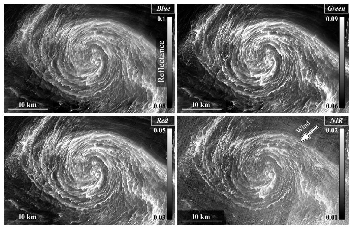
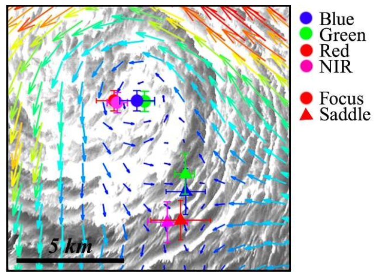
Figure 1. Map of satellite imaging of the Baltic Sea on 25 July 2018; blue area: Landsat-8 OLI, green area: Sentinel 2A MSI. The fragments show the scenes in the green band.
Remotesensing 14 01871 g001
Figure 2. The studied fragment of the Sentinel 2A MSI scene in different bands. An arrow shows the wind direction.
Remotesensing 14 01871 g002
Figure 3. An example of the 1D cross-correlation coefficient.
Remotesensing 14 01871 g003
Figure 4. Horizontal velocity field obtained using the MCC method (a), map of divergence (b) and vorticity (c), all for green band. The images depict the positions of zero-velocity points, see the legend.
Remotesensing 14 01871 g004aRemotesensing 14 01871 g004b
Figure 5. Graphical solution of the first equation of system (4).
Remotesensing 14 01871 g005
Figure 6. Horizontal streamlines scheme of the velocity field of a convergent eddy (a) and of the velocity field consisting of an eddy and a homogeneous drift current directed opposite to the y-direction (b). Grey area, the eddy core; the red and greed dots depict the positions of a focus and a saddle.
Remotesensing 14 01871 g006
Figure 7. Positions of the points of zero velocity in different bands.
Remotesensing 14 01871 g007
Figure 8. Velocity field after the subtraction of the mean drift component (green band); the scales of eddy core boundaries with corresponding maximal tangential velocities are indicated by black lines.
Remotesensing 14 01871 g008
Table 1. Wavelengths of the studied bands and corresponding mean horizontal velocities.
BandWavelength (Landsat-8 OLI), nmWavelength (Sentinel 2A MSI), nm<Vx>, cm/c<Vy>, cm/c
Blue0.45–0.5150.448–0.545−16.4−7.2
Green0.525–0.60.537–0.582−14.9−7
Red0.63–0.680.645–0.683−16.5−4.5
NIR0.845–0.8850.848–0.883−18.1−6.6
Publisher’s Note: MDPI stays neutral with regard to jurisdictional claims in published maps and institutional affiliations.

