A Method for Digital Terrain Reconstruction Using Longitudinal Control Lines and Sparse Measured Cross Sections

Abstract

Using longitudinal control lines and sparse measured cross sections with large spaces, a new method for quickly reconstructing digital terrains in natural riverways is presented. The longitudinal control lines in a natural riverway, mainly including the river boundaries, the thalweg, the dividing lines of floodplains and main channel, and the water edges, can be obtained by interpreting satellite images, remote sensing images or site surveys. Then, the longitudinal control lines are introduced into quadrilateral grid generation as auxiliary lines that can control longitudinal riverway trends and reflect transverse terrain changes. Then, by the equal cross-sectional area principle at the same water level, all measured cross sections are reasonably fitted. On the above basis, by virtue of the fitted cross-sectional data and the weighted distance method, the terrain interpolations along the longitudinal grid lines are conducted to obtain the elevation data of all grid nodes. Finally, according to the readable text formats of MIKE21 and SMS, the gridded digital terrain and connection information are output by computer programming to achieve good construction of the data exchange channels and fully exploit the special advantages of various software programs for digital terrain visualization and further utilization.

1. Introduction

In river numerical simulations, whether the elevation values at grid nodes can truthfully reflect the riverway terrain is very important, as it directly determines the reliability of numerical simulation results [1,2,3]. In the process of riverway terrain reconstruction, to guarantee the truth and reasonability of the reconstruction results, many types of river numerical software are required to provide a large amount of terrain data covering the simulation areas and uniformly distributed. Due to the long terrain measurement period and large investment, under most situations, the method of laying uniform measured points for the whole riverway is not used in practical surveys. Generally, only the cross-sectional terrain data with large spaces are measured [4]. If entirely relying on the interpolation functions of conventional software to construct a riverway mode, the terrain accuracy will be low, and the accuracy and credibility of the numerical simulation results will be difficult to ensure. Therefore, it is necessary to explore a terrain reconstruction method for the sparsely measured cross-sectional data.

In the early studies, many scholars were keen to develop new methods. For example, Lin et al. [5] proposed a method of automatically reconstructing three-dimensional objects by a series of cross sections. Hardy [6] proposed the radial basis function interpolation algorithm, which has been widely used in many fields such as terrain modeling and digital approximation, but as the number of sampled points increases, the solution speed of the radial basis function interpolation model greatly decreases. Targeting the deficiency of the radial basis function interpolation algorithm, some scholars presented the residual iteration method [7], quick multipolarization method [8] and partition of unity method [9], providing quick and accurate solutions for the radial basis function interpolation model from different aspects. Yokota et al. [10] conducted parallel processing of the radial basis function interpolation algorithm to improve the terrain reconstruction ability. Yang et al. [11] proposed a new method to achieve cross-sectional interpolation and evaluation deduction by curved surface interpolation technology. A weighted interpolation algorithm was presented by Wagner et al. [12] for reconstructing the cross-sectional profiles. Caviedes-Voullieme et al. [13] presented a new algorithm for generating missing information between the cross sections and the riverbed. Lebrenz and Bardossy [14] proposed a quantile kriging interpolation method, which needs to estimate variable distribution with time at the observed sites, as well as the marginal distribution in each predetermined time step. Due to the unremitting efforts of the above scholars, there are many terrain reconstruction methods. The proposal of a new method is obviously a breakthrough, but its calculational accuracy is also worthy of paying enough attention. Therefore, some scholars strictly compare the calculational accuracies of the existing terrain reconstruction methods. For instance, Weber [15] believed that the interpolation effects of the radial basis function algorithm and the inverse distance weighted method are basically the same. Kraus [16] thought that the interpolation effect of multilayer curved surface superposition is better than that of the binary higher-degree polynomial and spline functions. Zimmerman et al. [17] pointed out that, without consideration of the terrain type and sampling method, the interpolation effect of the kriging interpolation algorithm is better than that of the inverse distance weighted method. Gichamo et al. [18] found correcting the vertical bias of elevation points by a high-accuracy terrain model can considerably improve the cross-sectional obtainment. Andes et al. [19] thought that the rectilinear inverse distance weighting methodology is fairly feasible for cross-sectional interpolation. Determining the optimal algorithm is undoubtedly an effective means to improve the calculational accuracy, but a single method cannot meet all the needs of terrain reconstruction, because the calculational accuracy depends not only on the algorithm itself, but also on the geomorphic type and sampling density. Therefore, some scholars started to deeply discuss the effects of geomorphic type and sampling density on calculational accuracy. For example, based on regular discrete point data, by analyzing the influence of the geomorphic type, sampling density and interpolation algorithm on the regular grid digital terrain interpolation, Aguilar et al. [20] concluded that the effect of the geomorphic type on the digital terrain interpolation is largest, that of the sampling density is the second, and that of the interpolation algorithm is smallest. In addition, a few scholars focused on the application of terrain reconstruction result. For instance, Chen et al. [21] pointed out that the appropriate use of the interpolated cross sections can increase the precision of hydraulic river models. Florinsky et al. [22] analyzed the spatial distribution of soil properties by the regression analysis of topographic data. Applying elevation data and satellite remote sensing data, Sun et al. [23] established a riverway digital elevation model using a curved orthogonal grid and calculated the silt dash quantity of the riverway.

When the terrain data are relatively conventional, the measured point distribution is uniform and the sampling density is large, the calculational accuracies of many ready-made terrain reconstruction methods can meet the actual production requirements. However, for the terrain data in natural rivers, the situation is fairly different. The terrain changes of a natural riverway are neither isotropic nor completely anisotropic, but have very distinct transverse and longitudinal spatial tropisms. The spatial tropisms can be indirectly reflected by the longitudinal control lines such as the river boundaries, the thalweg, the dividing lines of floodplains and main channel, the water edges, etc. In other words, the longitudinal control lines have a function of controlling the longitudinal riverway trends and reflecting the transverse terrain changes. Nevertheless, this special function of the longitudinal control lines has not been paid enough attention by the engineering surveyors for a long time. In all previous studies, the spatial tropisms between an interpolated point and the adjacent elevation points have not been fully considered when constructing the interpolation weights. Especially in a natural riverway where the transverse and longitudinal terrain changes present obviously different spatial tropisms, if the spatial tropisms between an interpolated point and the adjacent elevation points are not considered, the terrain interpolation accuracy will inevitably be affected when constructing the river digital model. Furthermore, for a natural riverway, there are only sparse measured cross-sectional data in most situations, which often does not meet the calculational requirements of many ready-made terrain reconstruction methods, let alone guarantee the reliabilities of the calculated results. For the above stated reasons, a new method for quickly reconstructing riverway digital terrains using longitudinal control lines and sparse measured cross sections with large spaces is presented.

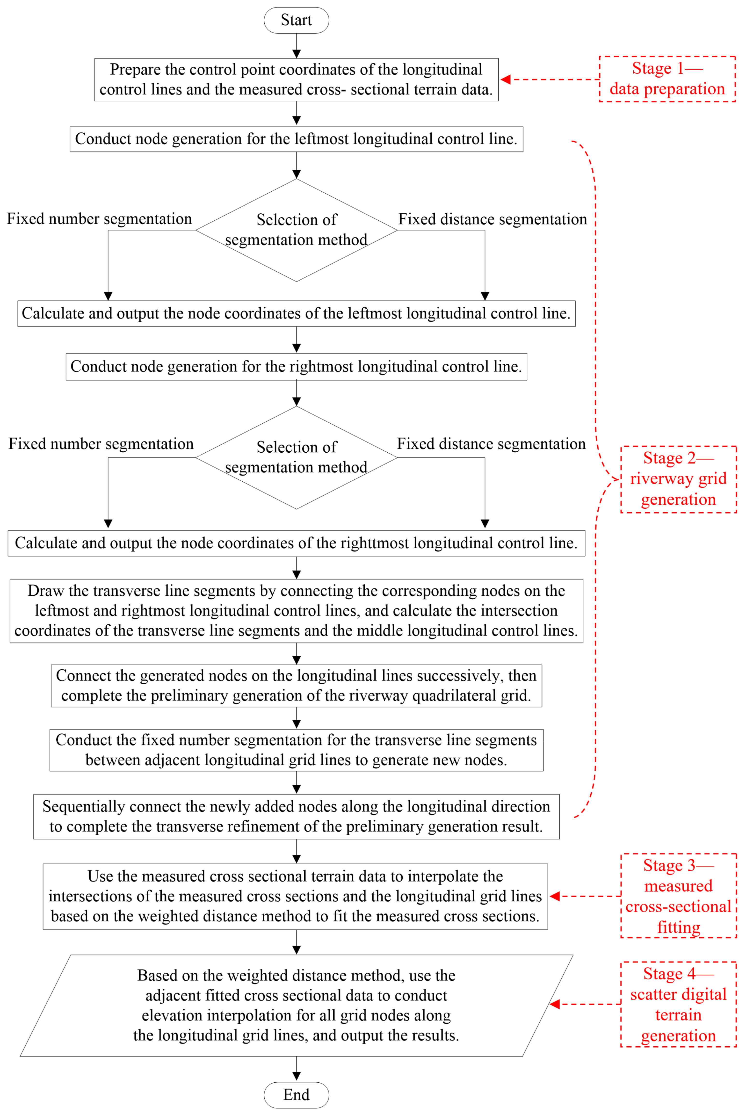
2. Digital Terrain Reconstruction Method

Digital terrain reconstruction for a natural riverway refers to utilizing a small number of sparse measured cross-sectional data to generate the dense scatter terrain data of the target riverway by an interpolation method. The method presented in this paper also belongs to this case, and its specific process can be roughly divided into four stages (in Figure 1).

Figure 1. Digital terrain reconstruction process.

Stage 1—data preparation: the plane coordinate data of the longitudinal control lines and the measured cross-sectional terrain data must be prepared first.

Stage 2—riverway grid generation: the longitudinal control lines are introduced into the process of quadrilateral grid generation so that the generated grid can be well adapted to the riverway boundary changes, controlling the longitudinal riverway trends and reflecting the transverse terrain changes.

Stage 3—measured cross-sectional fitting: the measured cross-sectional terrain data are used to interpolate the intersections of the measured cross sections and the longitudinal grid lines by the equal cross-sectional area principle at a same water level and weighted distance method to reasonably fit the measured cross sections.

Stage 4—scatter digital terrain generation: using the generalized cross-sectional data and the weighted distance method, the elevation interpolations of all grid nodes are conducted along longitudinal grid lines to generate the whole riverway digital terrain. The detailed digital terrain reconstruction process can be seen in following contents.

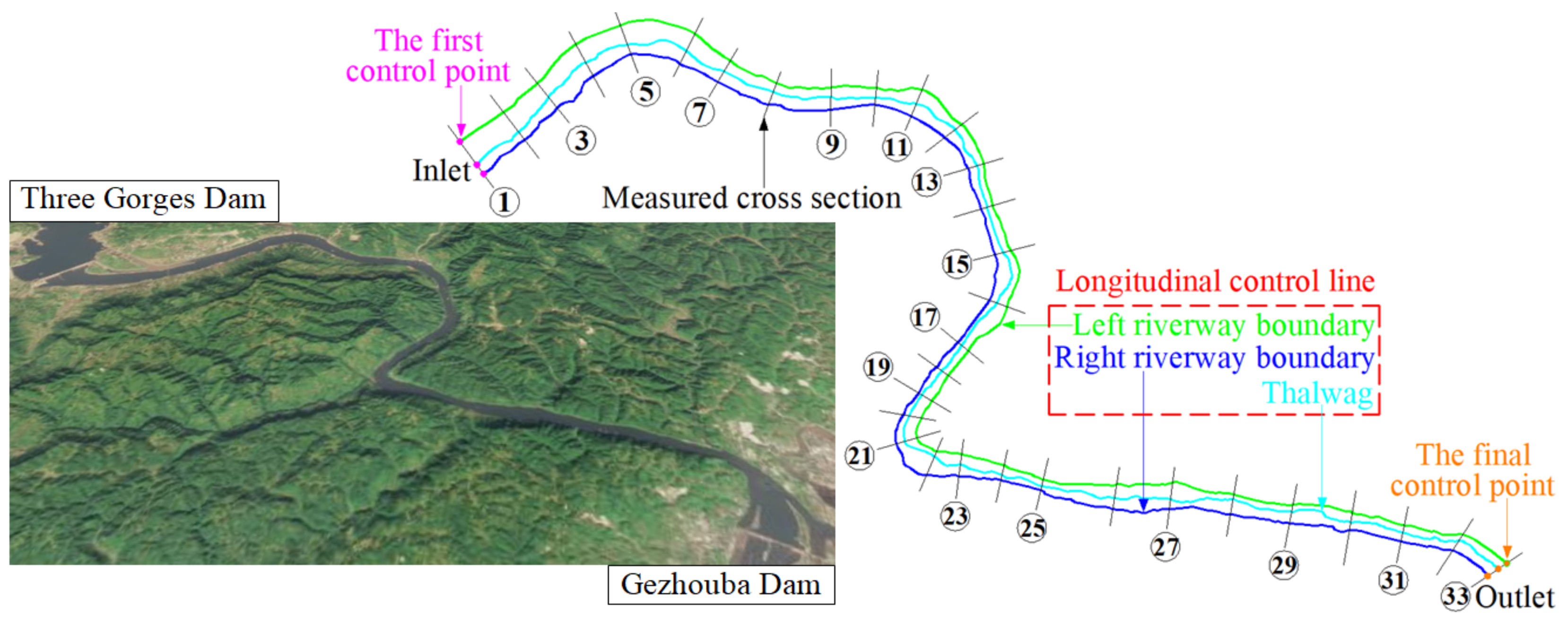
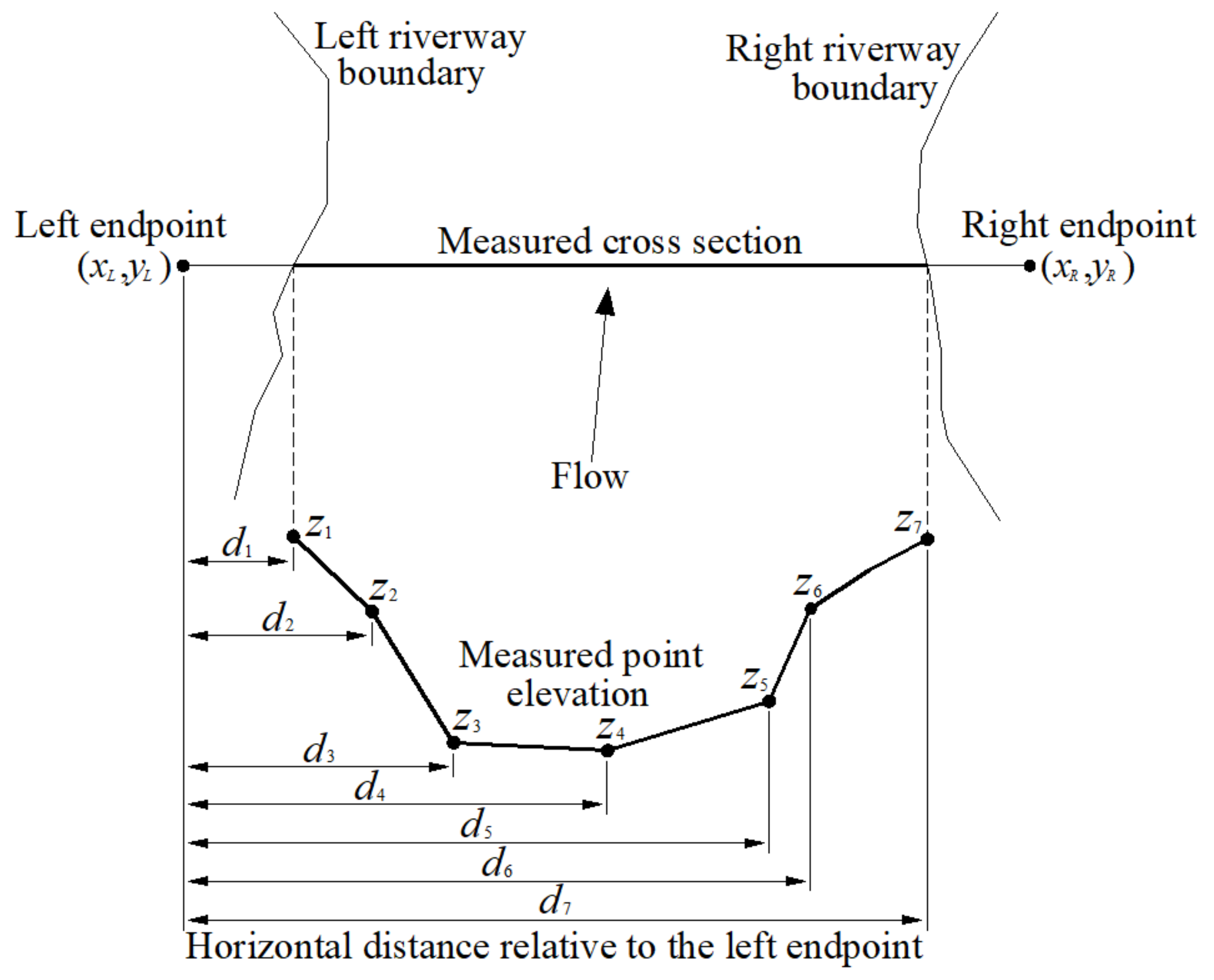
2.1. Data Preparation

Before the digital terrain reconstruction for a natural riverway, the plane coordinate data of the longitudinal control lines and the measured cross-sectional terrain data must be prepared first.

The longitudinal control line data are actually a series of sequential plane control points, which can determine the plane shapes of the longitudinal control lines and can be obtained by interpreting satellite images, remote sensing images or site surveys [24,25,26,27,28,29]. As shown in Figure 2, for any a longitudinal control line, the first control point and the final control point are the intersections of the inlet measured cross section, the outlet measured cross section and the longitudinal control line. If the effects of river control works, production dikes and other engineering boundaries need to be considered, the positional coordinates of the engineering boundaries should be provided. In addition, It should be pointed out that this method does not require the acquisition of too many longitudinal control lines, but generally speaking, the more the number of the used longitudinal control lines is, the more accurate the calculated result is.

Figure 2. Distributions of longitudinal control lines and measured cross sections (The exemplified riverway is located between the Three Gorges Dam and Gezhouba Dam in China and approximately 30 km in length. The distances between the adjacent sections are approximately 600~1100 m).

The measured cross-sectional terrain data mainly include the cross-sectional left and right endpoint coordinates (the left and right sides are defined according to the flow direction), the measured point elevations and the horizontal distances between the measured points and the corresponding left endpoint (in Figure 3).

Figure 3. Schematic sketch of the measured cross-sectional data.

In this paper, a natural riverway, which is located between the Three Gorges Dam and Gezhouba Dam in China and approximately 30 km in length (in Figure 2), is used to briefly describe the digital terrain reconstruction process. In the early stage, 33 sparse measured cross sections and 3 longitudinal control lines (the left riverway boundary, the right riverway boundary and the thalweg) of the exemplified riverway were obtained through peer collection, visual judgment of satellite images and field survey, therein the distances between the adjacent measured cross sections are approximately 600~1100 m.

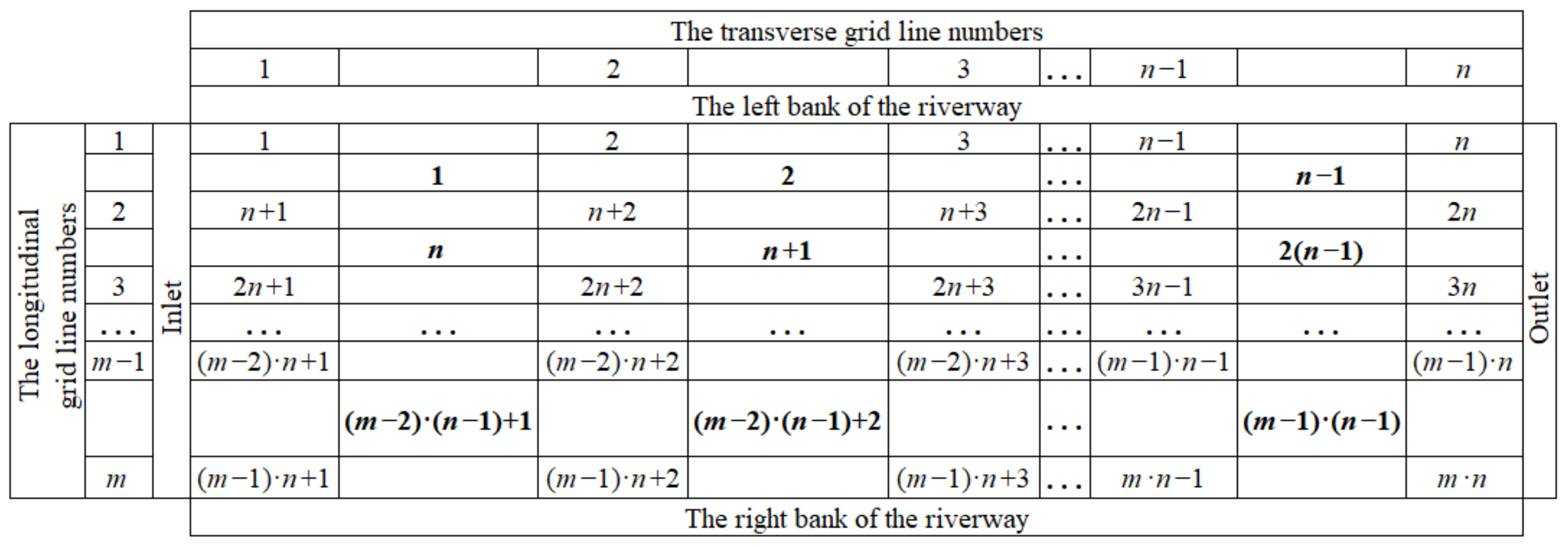
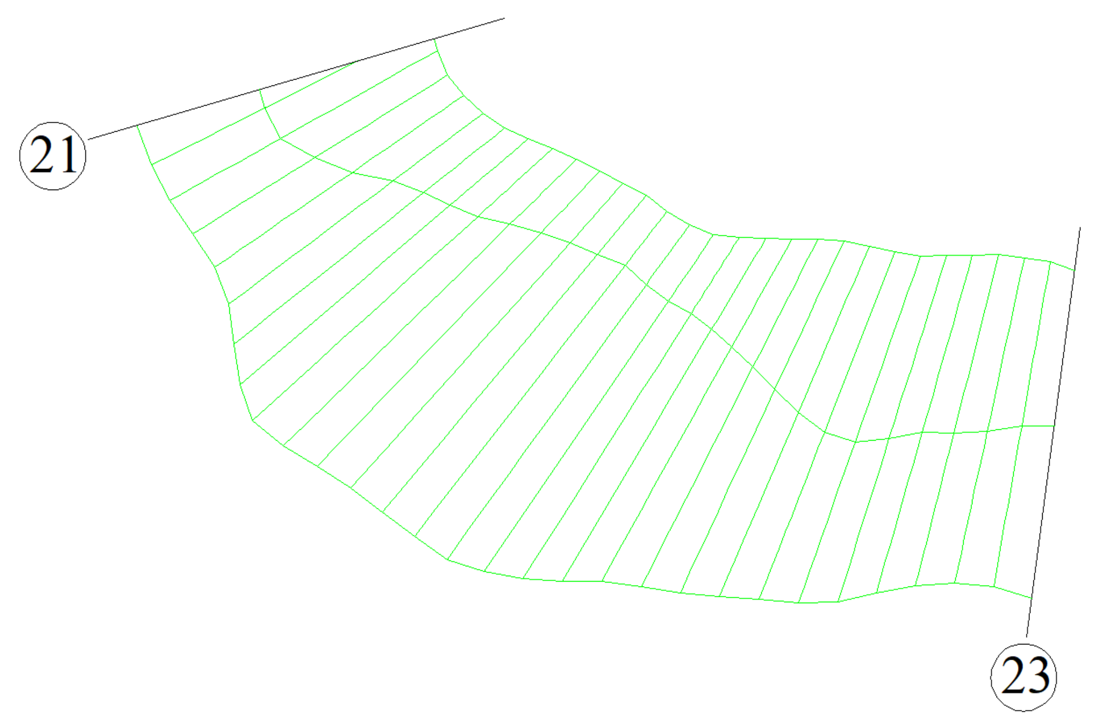
2.2. Riverway Grid Generation

In this paper, quadrilateral cells are used to conduct the grid generation for the target river reach. Riverway grid generation is an important process in the digital terrain reconstruction, and its specific process can be roughly divided into five steps.

Step 1—cumulative distance calculation for the riverway boundary control points.

Step 2—node generation for the left riverway boundary.

Step 3—node generation for the right riverway boundary.

Step 4—preliminary grid generation.

Step 5—transverse refinement for the preliminary grids.

2.2.1. Cumulative Distance Calculation for the Riverway Boundary Control Points

For generating riverway grids, the cumulative distances of the riverway boundary control points relative to the corresponding first control points should be firstly calculated. Assuming that the control point number of the left riverway boundary is $N_L$, if the cumulative distance of the first control point relative to itself is recorded as 0 and the serial number is 1, then the plane coordinates and cumulative distances of the control points on the left riverway boundary can be combined into $(x_L(i),y_L(i),L_L(i))$ where $i=1,2,3,\dots ,N_L$, therein $L_L(1)=0$. Similarly, assuming that the control point number of the right riverway boundary is $N_R$, then the plane coordinates and cumulative distances of the control points on the right riverway boundary can be combined into $(x_R(i),y_R(i),L_R(i))$ where $i=1,2,3,\dots ,N_R$, therein $L_R(1)=0$. Actually, for any a longitudinal control line, the cumulative distance of the final control point relative to the first control point is equal to the total length of the longitudinal control line, and the difference between two adjacent cumulative distances is the distance between the two corresponding control points.

2.2.2. Node Generation for the Left Riverway Boundary

After the cumulative distances of the boundary control points relative to the corresponding first control points are calculated and stored in the sequential data format, node generation could be conducted for the left riverway boundary. Here, the fixed number segmentation method or the fixed distance segmentation method may be selected.

Assuming the fixed number segmentation method is selected and $n_L$ is taken as the segmentation number, then the generation step size $s_L$ along the left river boundary is equal to $L_L(N_L)/n_L$, and finally $n_L+1$ nodes could be generated. According to the cumulative distances, the left riverway boundary is divided into $N_L-1$ cumulative distance intervals, namely $\left[L_L(1),L_L(2)\right]$, $\left[L_L(2),L_L(3)\right]$$,\dots ,$ $\left[L_L(N_L-1),L_L(N_L)\right]$. Then, taking the first control point as the starting point, the stepping distances $j·s_L (j=0,1,2,\dots ,n_L)$ along the left riverway boundary could be successively calculated. If a stepping distance $j·s_L$ falls in the cumulative distance interval $[L_L(k),L_L(k+1)]$, namely $L_L(k)\le j·s_L \le L_L(k+1)$, then the node coordinate $\left(x_{L,\mathrm{n}\mathrm{o}\mathrm{d}\mathrm{e}}(j+1),y_{L,\mathrm{n}\mathrm{o}\mathrm{d}\mathrm{e}}(j+1)\right)$ can be calculated according to Formulas (1) and (2).

$$x_{\xi ,\mathrm{n}\mathrm{o}\mathrm{d}\mathrm{e}}(j+1)=\frac{(j·s_{\xi }-L_{\xi }(k))·(x_{\xi }(k+1)-x_{\xi }(k))}{\sqrt{{(x_{\xi }(k+1)-x_{\xi }(k))}^2+{(y_{\xi }(k+1)-y_{\xi }(k))}^2}}+x_{\xi }(k)$$

(1)

$$y_{\xi ,\mathrm{n}\mathrm{o}\mathrm{d}\mathrm{e}}(j+1)=\frac{(j·s_{\xi }-L_{\xi }(k))·(y_{\xi }(k+1)-y_{\xi }(k))}{\sqrt{{(x_{\xi }(k+1)-x_{\xi }(k))}^2+{(y_{\xi }(k+1)-y_{\xi }(k))}^2}}+y_{\xi }(k)$$

(2)

where the subscript $\xi$ is equal to L or R; when $\xi =L$, the above formulas are used to calculate the node coordinates of the left river boundary; when $\xi =R$, the above formulas are used to calculate the node coordinates of the right river boundary.

Assuming the fixed distance segmentation method is selected and $L_{0,L}$ is taken as the segmentation distance, then the generation step size $s_L$ along the left river boundary is equal to $L_{0,L}$, but the generated node amount is relevant to the segmentation distance $L_{0,L}$. When the remainder of $L_L(N_L)/L_{0,L}$ is equal to 0, the fixed distance segmentation method is equivalent to the fixed number segmentation method whose segmentation number $n_L$ equals $L_L(N_L)/L_{0,L}$, and finally $L_L(N_L)/L_{0,L}+1$ nodes could be generated, and the node coordinates $(x_{L,\mathrm{n}\mathrm{o}\mathrm{d}\mathrm{e}}(j+1),y_{L,\mathrm{n}\mathrm{o}\mathrm{d}\mathrm{e}}(j+1))$ ($j=0,1,2,\dots ,L_L(N_L)/L_{0,L}$) can be successively calculated according to Formulas (1) and (2). When the remainder of $L_L(N_L)/L_{0,L}$ is not equal to 0, the segmentation number $n_L$ equals $[L_L(N_L)/L_{0,L}]+1$ where $[L_L(N_L)/L_{0,L}]$ represents that only the integral part of $L_L(N_L+1)/L_{0,L}$ is used, and finally $[L_L(N_L)/L_{0,L}]+2$ nodes could be generated. Therein, the first $[L_L(N_L)/L_{0,L}]+1$ node coordinates $(x_{L,\mathrm{n}\mathrm{o}\mathrm{d}\mathrm{e}}(j+1),y_{L,\mathrm{n}\mathrm{o}\mathrm{d}\mathrm{e}}(j+1))$ ($j=0,1,2,\dots ,[L_L(N_L)/L_{0,L}]$) can be successively calculated according to Formulas (1) and (2), and the final control point of the left riverway boundary is actually the final node.

2.2.3. Node Generation for the Right Riverway Boundary

The next step, node generation is conducted for the right riverway boundary. Here, the fixed number segmentation method or the fixed distance segmentation method may be selected. As the generated grid cells in the target river reach are quadrilateral, the segmentation number of the right riverway boundary must be equal to that of the left riverway boundary, namely $n_R=n_L$.

Assuming the fixed number segmentation method is selected and the segmentation number is $n_R$, then the generation step size $s_R$ along the right river boundary is equal to $L_R(N_R)/n_R$, and finally $n_R+1$ nodes could be generated. Here, the calculational method of the node coordinates likes the left river boundary when the fixed number segmentation method is selected. Only at this time, the subscript $\xi$ in Formulas (1) and (2) is equal to R.

Assuming the fixed distance segmentation method is selected, then the segmentation distance $L_{0,R}$ must be within $[L_R(N_R)/n_R, L_R(N_R)/(n_R-1)]$ to guarantee $n_R=n_L$, and the generation step size $s_R$ is equal to $L_{0,R}$, and finally $n_R+1$ nodes are generated. If $L_{0,R}=L_R(N_R)/n_R$, the calculational method of the node coordinates likes the left river boundary when the fixed distance segmentation method is selected and the remainder of $L_L(N_L)/L_{0,L}$ is equal to 0. If $L_R(N_R)/n_R<L_{0,R}<L_R(N_R)/(n_R-1)$, the calculational method of the node coordinates likes the left river boundary when the fixed distance segmentation method is selected and the remainder of $L_L(N_L)/L_{0,L}$ is not equal to 0.

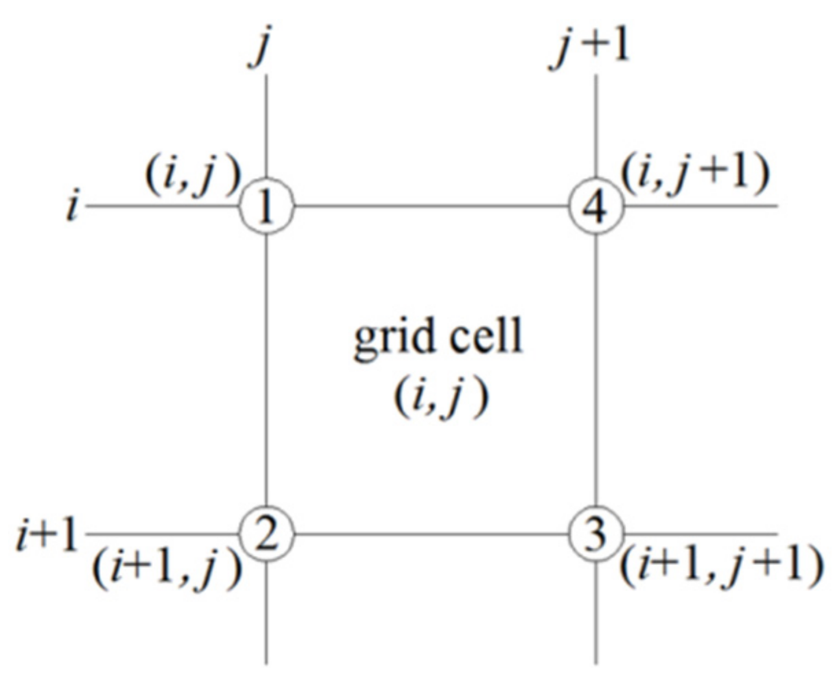
2.2.4. Preliminary Grid Generation

After the node generation of the riverway boundaries, the corresponding nodes on the left and right riverway boundaries are first connected along the transverse directions. Then, the intersection coordinates of the connected line segments and the thalweg are calculated to complete the node generation of the thalweg. Finally, the generated nodes are connected successively along the longitudinal direction. At this point, the preliminary quadrilateral grid generation in the target reach is completed. However, due to the small number of longitudinal control lines, the transverse spaces of the longitudinal grid lines are large (in Figure 4).

Figure 4. Preliminary generation result of quadrilateral grids (In the exemplified preliminary grid generation, the fixed number segmentation method is applied to the riverway boundaries).

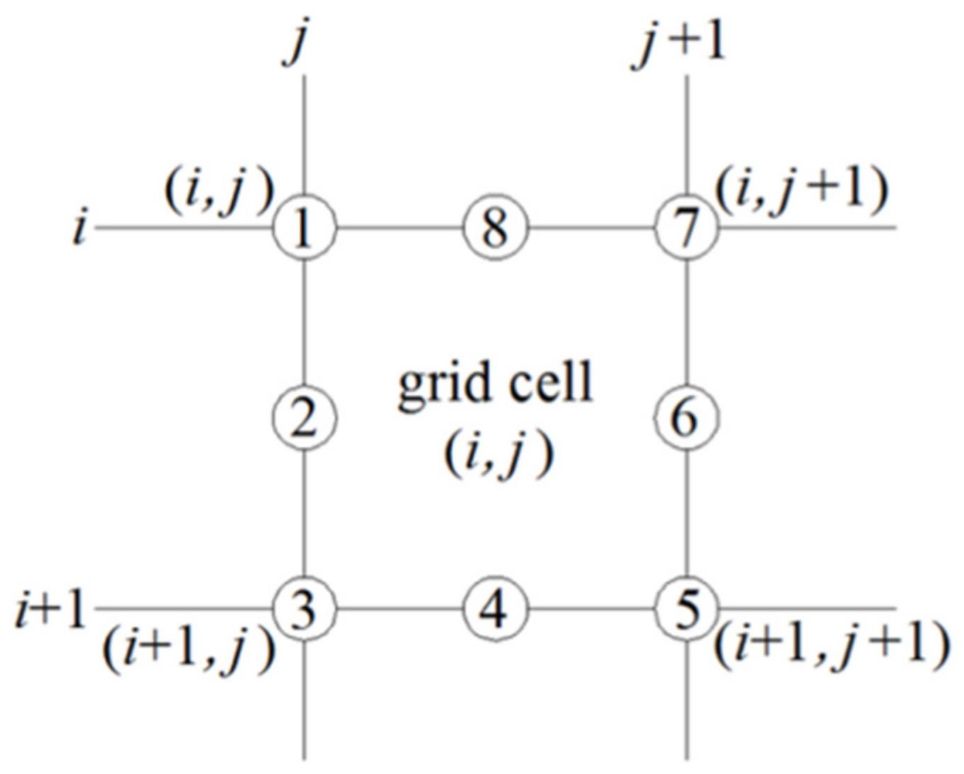
2.2.5. Transverse Refinement for the Preliminary Grids

To decrease the transverse spaces between adjacent longitudinal grid lines, the transverse line segments between adjacent longitudinal grid lines must be subdivided. To ensure a uniform transverse density of the generated grids, the transverse line segments between any two adjacent longitudinal grid lines must be divided by the fixed number segmentation method. The segmentation numbers between different adjacent longitudinal grid lines can be different, but those between the same adjacent longitudinal grid lines must be the same, and the specific values should be determined according to the transverse spaces between the adjacent longitudinal grid lines. The larger the transverse spaces are, the larger the segmentation numbers should be. Then, the newly added nodes are successively connected along the longitudinal direction. After the adding line operations are conducted in the regions between any two adjacent longitudinal grid lines, the transverse refinement of the preliminary generation result is completed (in Figure 5).

Figure 5. Transverse refinement effect of the preliminary grids and elevation interpolation schematic by the weighted distance method (In the process of the illustrative transverse refinement, the transverse segmentation numbers between the adjacent longitudinal control lines from the left side to right side are all 10).

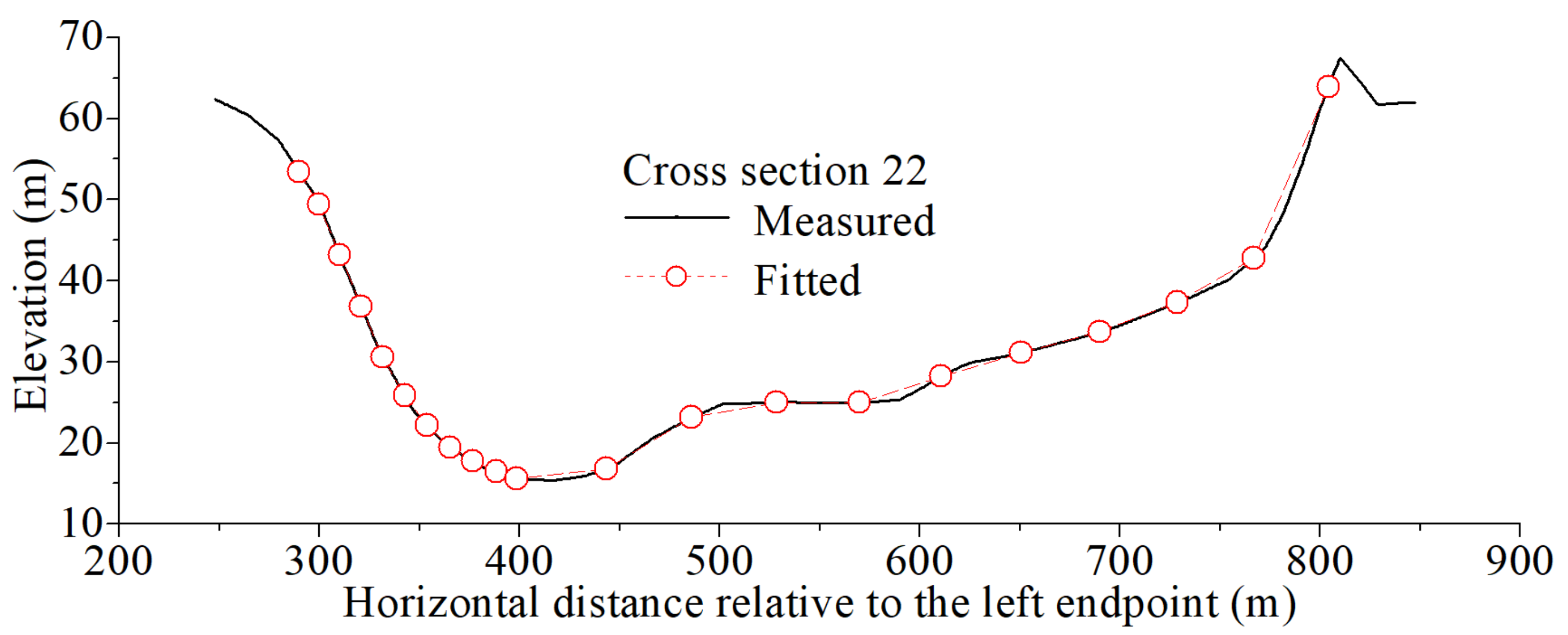
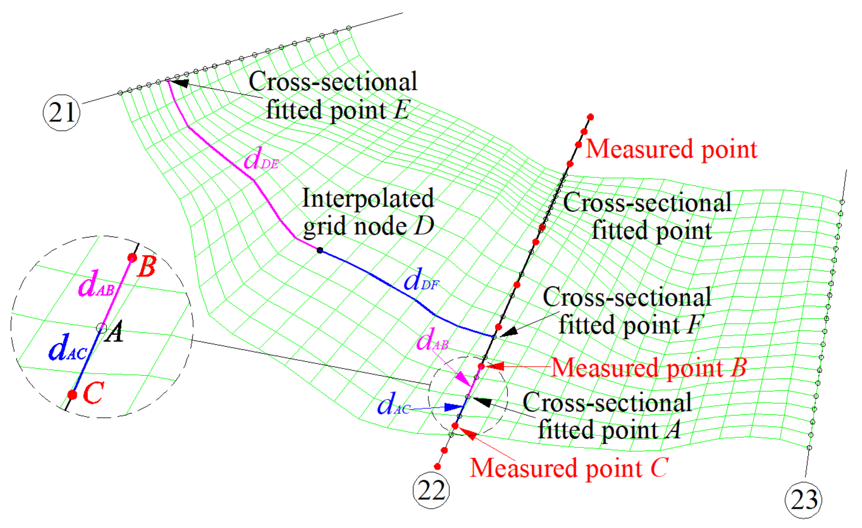
2.3. Measured Cross-Sectional Fitting

After the grid generation in the target river reach is completed, the intersection coordinates of each measured cross section and the longitudinal grid lines could be calculated and translated into the horizontal distances relative to the measured cross-sectional left endpoint. Then, the measured cross-sectional data are used to interpolate the intersections of the measured cross sections and the longitudinal grid lines by the weighted distance method to reasonably fit the measured cross sections (Figure 6 only shows the 22nd cross section). The weighted distance method is an interpolation method based on the similarity principle, and it constructs the interpolation weights by the distances between the interpolated point and the sampled points. The shorter the distance between the interpolated point and a sampled point is, the greater the weight granted by the sampled point. In this step, the specific interpolation process is as follows: As shown in Figure 5, for a cross-sectional fitted point A and two measured points B and C, which are located in the same cross section as that of point A and are closest to point A, if the elevations of points B and C are $z_B$ and $z_C$, and the distances between A and points B and C are, respectively, $d_{AB}$ and $d_{AC}$, then the elevation $z_A$ of point A can be calculated according to Formula (3).

$$z_A=d_{AC}·z_B/(d_{AB}+d_{AC})+d_{AB}·z_C/(d_{AB}+d_{AC})$$

(3)

Figure 6. Measured cross-sectional fitting.

The rationality of measured cross-sectional fittings directly determines the accuracy of the reconstructed riverway digital terrain. The most ideal situation is that the fitted shapes of the measured cross sections are entirely consistent with the actual cross-sectional terrains. In other words, at th same water level, a fitted cross section and the corresponding measured cross section have same cross-sectional parameters (mainly including cross-sectional area, wetted perimeter, hydraulic radius, water surface width and average water depth), which is referred to as the equal cross-sectional area principle. The good or bad actual fitting effects are directly relevant to the selective rationality of the longitudinal control lines and the transverse spaces of the generated grids. When the selection of the longitudinal control lines in a target riverway is reasonable and the transverse spaces of the generated grids are small, the fitted cross sections are usually close to the actual cross-sectional terrain. If judging the rationality of the fitted cross sections is necessary, the cross-sectional parameters of the measured cross sections and the fitted cross sections under a series of water level conditions can be calculated for comparison.

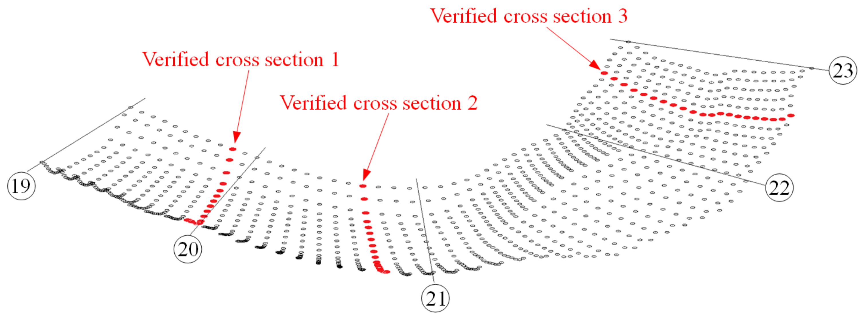
2.4. Scatter Digital Terrain Generation

After the measured cross sections are reasonably fitted, the elevation interpolations of the grid nodes can be conducted along the longitudinal grid lines by the adjacent fitted cross sections and the weighted distance method, and the whole riverway digital terrain can be generated (in Figure 7). In this step, the specific interpolation process is as follows: As shown in Figure 5, assuming that the interpolated grid node is D, the two cross-sectional fitted points with known elevations and the closest longitudinal distances relative to point D are E and F, and point D is located in the middle of points E and F, and the elevations of points E and F are, respectively, $z_E$ and $z_F$, and the longitudinal distances between D and points E and F are, respectively, $d_{DE}$ and $d_{DF}$, then the elevation $z_D$ of point D can be calculated according to Formula (4).

$$z_D=d_{DF}·z_E/(d_{DE}+d_{DF})+d_{DE}·z_F/(d_{DE}+d_{DF})$$

(4)

Figure 7. Riverway scattered digital terrain.

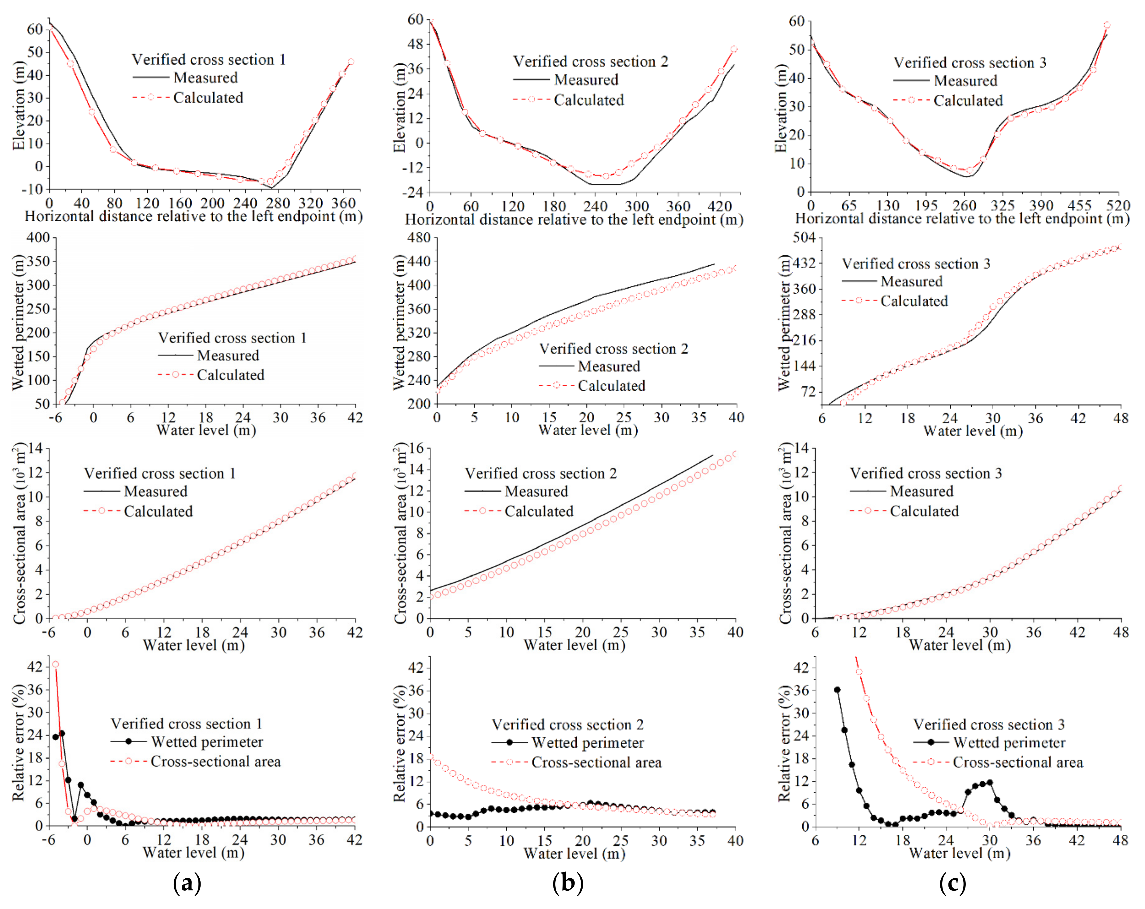
3. Comparisons between the Measured and Calculated Results

To verify the reasonableness of the calculated results, authors conducted a supplementary measurement for the actual terrains of the three verified cross sections (in Figure 7). Through a comparison of the calculated results with the measured results of the three verified cross sections, it can be found that the calculated results are be close to the measured results in cross-sectional shape, and the relative errors ($relative error=\left|calculated X-measured X\right|/measured X$) of the calculated cross-sectional areas and the calculated wetted perimeters may reach more than 40% at a low water level, but smaller than 5% at a moderate water level (in Figure 8). In river simulation, if the relative error between the constructed riverway model and the actual terrain is not more than 5%, we usually believe that the constructed river model meets the calculational accuracy requirements [23,30]. This means that at a moderate water level, the method presented in this paper is accurate enough to meet the terrain accuracy requirements in actual production. For the exemplified riverway, why the relative errors of the calculated results are large at a low water level is due to the small number of the used longitudinal control lines and the large grid spaces. In this paper, three longitudinal control lines and large spaces are used for the riverway grid generation only to clarify the specific principle of the digital terrain reconstruction method in a concise way. In practical applications, if conditions permit, we should try our best to increase the numbers of the longitudinal control lines and the measured cross sections and choose small grid spaces as far as possible, which can further improve the calculational accuracy.

Figure 8. Comparisons between the measured and calculated results related to cross-sectional shape, wetted perimeter and cross-sectional area ((a) corresponding to the verified cross section 1; (b) corresponding to the verified cross section 2; (c) corresponding to the verified cross section 3).

4. Digital Terrain Applications

According to the readable text formats of MIKE21 and SMS, the gridded digital terrain and connection information are output by computer programming (such as Fortran, MATLAB, Python, etc.) to achieve good construction of the data exchange channels and fully exploit the special advantages of various software programs for digital terrain utilization.

4.1. Meshing Digital Terrain for MIKE21

MIKE is a flow simulation module developed by the Danish DHI Company that combines the widely used MIKE11 and MIKE21. MIKE21 is applicable to the argumentation and analysis of macroscopic watershed control engineering, the research on watershed flood dispatching, microscopic flow simulation and other fields. The common grid types include quadrilateral grids. The extension of the MIKE21 quadrilateral grid file is “mesh”, and its internal data include the node header line, the node lines, the cell header line, and the cell lines. The node header line is further divided into the entry type with integer form, the entry unit with integer form, the node amount and the character string of the projection type. The entry type is elevation, and its integer form is “100079”. The entry unit is the elevation unit, and the integer form “1000” indicates that the elevation values are stored in the z-coordinates and that their units are all meters. The third integer in the node header line is the node amount. The final string “NON-UTM” is the projection type. Each node line represents a node, and the total number of node lines is the same as the node amount in the node header line. The information of each node line includes the node number, x, y, z and boundary code. A boundary code of “0” represents the internal node, “1” represents the water-land boundary, “2” represents the inlet boundary, and “3” represents the outlet boundary. The three numbers in the cell header line indicate the cell amount, the maximum node amount in a single cell, and the cell type code (“25” represents a quadrilateral cell). Each cell line represents a cell, and the total number of cell lines is the same as the cell amount defined in the cell header line. The information in each cell line includes the cell number and the node numbers that constitute the cell.

To use the generated riverway terrain in the hydrodynamic module of MIKE21, it must be saved in the readable grid format of MIKE21 by computer programming. In the specific grid transformation process, the coding rules of the nodes and cells comply with the rules shown in Figure 9 (the bold values in the figure are the cell numbers, and the values at the four corners of the bold values are the node numbers). The node codes and the cell codes are conducted from the riverway inlet to the outlet along the longitudinal grid line, and the transverse output sequence starts from the left bank of the riverway and ends at the right bank. Assume that the number of generated longitudinal grid lines is m, the number of generated transverse grid lines is n, the numbering sequence of longitudinal grid lines is from left to right, and the numbering sequence of transverse grid lines is from the inlet to the outlet (in Figure 9). When each longitudinal grid line is regarded as a row, each transverse grid line is regarded as a column, the row number is indicated by i, the column number is indicated by j, and the cell is indicated by the combination (i, j) of the smallest row number and the smallest column number of its four vertices, then a one-to-one correspondence exists among the cell number, the node numbers constituting the cell, and the transverse and longitudinal grid line numbers. As shown in Figure 10, when the row and column number combination of a certain cell is (i, j) where i = 1, 2, …, m − 1 and j = 1, 2, …, n − 1, the cell number is calculated as (i − 1)·(n − 1) + j. If the nodes constituting the cell are recorded as ➀, ➁, ➂, and ➃ along the counterclockwise direction, then the node numbers can be calculated according to formula sets (5). If the cell number is N, the row and column number combination (i, j) of the cell can also be calculated, where i is the minimum integer not less than N/(n − 1), and j equals N − (i − 1)·(n − 1). After i and j are calculated, the corresponding node numbers can be obtained by substituting i and j into formula sets (5).

$$\left\{\begin{array}{l}➀:j+(i-1)·n\\ ➁:j+i·n\\ ➂:j+1+i·n\\ ➃:j+1+(i-1)·n\end{array}\right.$$

(5)

Figure 9. Coding rules of nodes and cells in the MIKE21 quadrilateral grid file (The rows marked “1, 2, …, m” represent longitudinal grid lines; the columns marked “1, 2, …, n” represent longitudinal grid lines; the bold values in the figure are the cell numbers; and the values at the four corners of the bold values are the node numbers.).

Figure 10. Numbering calculation of nodes constituting a MIKE21 quadrilateral grid cell (“i” and “i + 1” represent the serial numbers of the adjacent longitudinal grid lines; “j” and “j + 1” represent the serial numbers of the adjacent transverse grid lines; the cell serial number is marked by the combination (i, j); and “➀~➃” are the node numbers constituting the cell).

When the readable grid file of MIKE21 is generated using the above rules by means of computer programming, it can be imported into the hydrodynamic module of MIKE21 to conduct the numerical simulation. After the grid file is imported into the stated module, the colored terrain map is as shown in Figure 11.

Figure 11. Terrain colored map based on MIKE21.

4.2. Meshing Digital Terrain for SMS

The surface water modeling system (referred to as SMS) is a business software program jointly developed by the United States Army Corps of Engineers Hydraulics Laboratory and Brigham Young University. Its quadrilateral grid file extension is “2 dm”, and its internal data mainly include a cell line, node line and node strings indicating the open boundaries (inlet and outlet boundaries). The cell lines begin with “E8Q” and are followed by the cell number, the node numbers constituting the cell (a quadrilateral cell in SMS consists of eight nodes—four vertices and the midpoints of four edges) and the material number. Each node line begins with “ND” and is followed by the node number, x and y coordinates, and elevation. The node strings indicating the open boundaries begin with “NS” and are followed by the node numbers of constituting the node strings. The numbering sequence generally starts from the right bank of the riverway and ends with a negative number.

To use the generated riverway terrain in the two-dimensional flow and sediment transport module of SMS, it must be saved in the readable grid format of SMS by computer programming. However, since a quadrilateral cell in the SMS readable grid format includes eight nodes (four vertices and the midpoints of four edges), only the vertex coordinates of the quadrilateral grid cells are obtained by the abovementioned method. Therefore, before grid conversion, the midpoint coordinates of the corresponding edges should be calculated based on the vertex coordinates of the quadrilateral grid cells. During the specific grid conversion, the coding rules of the nodes and cells can comply with the rules shown in Figure 12 (the bold values in the figure are the cell numbers, and the values around the bold values are the node numbers): First, the vertexes of each quadrilateral grid cell are encoded; second, the midpoints of the transverse edges are encoded; and finally, the midpoints of the longitudinal edges are encoded. The vertex codes and the midpoint codes of the transverse edges are conducted from the riverway inlet to the outlet along the longitudinal grid lines, and the transverse output sequence starts from the left bank and ends at the right bank. The midpoint codes of the longitudinal edges are conducted from the riverway left bank to the right bank along the transverse grid lines, and the longitudinal output sequence starts from the riverway inlet and ends at the outlet. The cell codes between two adjacent longitudinal grid lines start from the riverway inlet and end at the riverway outlet, and the transverse output sequence is from left to right along the transverse grid lines. Assume that the number of generated longitudinal grid lines is m, the number of generated transverse grid lines is n, the numbering sequence of longitudinal grid lines is from left to right, and the numbering sequence of the transverse grid lines is from the riverway inlet to the outlet (in Figure 12). If each longitudinal grid line is regarded as a row, each transverse grid line is regarded as a column, the row number is marked with i, the column number is marked with j, and the cell is marked by the combination (i, j) of the smallest row number and the smallest column number of its four vertices, then a one-to-one correspondence exists among the cell number, the node numbers constituting the cell, and the transverse and longitudinal grid line numbers. As shown in Figure 13, when the row and column number combination of a certain cell is (i, j) where i = 1, 2, …, m − 1 and j = 1, 2, …, n − 1, then the cell number is calculated as (i − 1)·(n − 1) + j. If the nodes constituting the cell are recorded as ➀, ➁, ➂, ➃, ➄, ➅, ➆ and ➇ along the counterclockwise direction, then the numbers can be calculated according to formula sets (6). If a cell number is known as N, the row and column number combination (i, j) of the cell can also be calculated, where i is the smallest integer not less than N/(n − 1) and j equals N − (i − 1)·(n − 1). After i and j are calculated, the corresponding node numbers can be obtained by substituting i and j into formula sets (6).

$$\left\{\begin{array}{l}➀:j+(i-1)·n\\ ➁:m·n+j+(i-1)·n\\ ➂:j+i·n\\ ➃:m·n+(m-1)·n+i-1+(j-1)·m\\ ➄:j+1+i·n\\ ➅:m·n+j+1+(i-1)·n\\ ➆:j+1+(i-1)·n\\ ➇:m·n+(m-1)·n+i+(j-1)·m\end{array}\right.$$

(6)

Figure 12. Coding rules of nodes and cells of the SMS quadrilateral grid file (The rows marked “1, 2, …, m” represent longitudinal grid lines; the columns marked “1, 2, …, n” represent longitudinal grid lines; the bold values in the figure are the cell numbers; and the values around the bold values are the node numbers).

Figure 13. Numbering calculation of nodes constituting an SMS quadrilateral grid cell (“i” and “i + 1” represent the serial numbers of the adjacent longitudinal grid lines; “j” and “j + 1” represent the serial numbers of the adjacent transverse grid lines; the cell serial number is marked by the combination (i, j); and “➀~➇” are the node numbers constituting the cell).

Using the above rules, after the readable grid file is generated by computer programming, it can be imported into the two-dimensional flow and sediment transport module of SMS to conduct the numerical simulation. After the grid file is imported into the stated module, the three-dimensional riverway grid can be obtained as shown in Figure 14.

Figure 14. Three-dimensional riverway grids based on SMS.

5. Conclusions

A new method for digital terrain reconstruction using longitudinal control lines and sparse measured cross sections with large spaces is presented. Through interpreting satellite images, remote sensing images or site surveys, the longitudinal control lines such as the river boundaries, the thalweg, the dividing lines of floodplains and main channel, the water edges, etc., can be obtained. Then, the longitudinal control lines are introduced into quadrilateral grid generation as auxiliary lines that can control longitudinal riverway trends and reflect transverse terrain changes. Then, using the equal cross-sectional area principle at a same water level and the weighted distance method, the elevation interpolations for the intersections of the measured cross sections and the longitudinal grid lines are carried out to reasonably fit the measured cross sections. On the above basis, the weighted distance method is used to interpolate all the grid nodes along longitudinal grid lines based on the fitted cross-sectional terrain data. Furthermore, the terrain elevations and connection information at the interpolated grid nodes can be output and integrated by computer programming according to the readable text formats of MIKE21, SMS or other software to achieve good construction of the data exchange channels and fully exploit the special advantages of various software programs for digital terrain visualization and further utilization. Overall, the physical conception of the digital terrain reconstruction method is clear, its implementation is simple and effective, and it is widely applicable to the digital terrain reconstructions in natural riverways using longitudinal control lines and sparse measured cross sections with large spaces.

References

- Bates, P.D.; Marks, K.J.; Horritt, M.S. Optimal use of high-resolution topographic data in flood inundation models. Hydrol. Process. 2003, 17, 537–557. [Google Scholar] [CrossRef]
- Horritt, M.S.; Bates, P.D.; Mattinson, M.J. Effects of mesh resolution and topographic representation in 2D finite volume models of shallow water fluvial flow. J. Hydrol. 2006, 329, 306–314. [Google Scholar] [CrossRef]
- Brasington, J.; Vericat, D.; Rychkov, I. Modeling river bed morphology, roughness, and surface sedimentology using high resolution terrestrial laser scanning. Water Resour. Res. 2012, 48, 1–18. [Google Scholar] [CrossRef] [Green Version]
- Castellarin, A.; Baldassarre, G.D.; Bates, P.D.; Brath, A. Optimal cross-sectional spacing in preissmann scheme 1D hydrodynamic models. J. Hydraul. Eng. 2009, 135, 96–105. [Google Scholar] [CrossRef]
- Lin, W.C.; Chen, S.Y.; Chen, C.T. A new surface interpolation technique for reconstructing 3D objects from serial cross-sections. Comput. Vis. Graph. Image Process. 1989, 48, 124–143. [Google Scholar] [CrossRef]
- Hardy, R.L. Theory and Applications of the Multiquadric-biharmonic Method 20 Years of Discovery 1968–1988. Comput. Math. Appl. 1990, 19, 163–208. [Google Scholar] [CrossRef] [Green Version]
- Beatson, R.K.; Cherrie, J.B.; Mouat, C.T. Fast fitting of radial basis functions: Methods based on preconditioned GMRES iteration. Adv. Comput. Math. 1999, 11, 253–270. [Google Scholar] [CrossRef]
- Carr, J.C.; Beatson, P.K.; Cherrie, J.B.; Mitchell, T.J.; Fright, W.R.; Mccallum, B.C.; Evans, T.R. Reconstruction and representation of 3D objects with radial basis functions. In Proceedings of the 28th Annual Conference on Computer Graphics and Interactive Techniques, New York, NY, USA, 28 July–1 August 2001. [Google Scholar]
- Zheng, H.; Song, L.; Hou, Y.; Hou, Y. The partition of unity parallel finite element algorithm. Adv. Comput. Math. 2015, 41, 937–951. [Google Scholar] [CrossRef]
- Yokota, R.; Barba, L.A.; Knepley, M.G. PetRBF-A Parallel O(N) algorithm for radial basis function interpolation with gaussians. Comput. Methods Appl. Mech. Eng. 2010, 199, 1793–1804. [Google Scholar] [CrossRef] [Green Version]
- Yang, M.; Liang, G.T.; Lai, R.X.; Yu, X. Theory and application of digital topography generation based on curved surface interpolation. J. Hydraul. Eng. 2007, 38, 221–225. (In Chinese) [Google Scholar]
- Wagner, B.; Gartner, H.; Santini, S.; Ingensand, H. Cross-sectional interpolation of annual rings within a 3D root model. Dendrochronologia 2011, 29, 201–210. [Google Scholar] [CrossRef]
- Caviedes-Voullieme, D.; Morales-Hernandez, M.; Lopez-Marijuan, I.; Garcia-Navarro, P. Reconstruction of 2D river beds by appropriate interpolation of 1D cross-sectional information for flood simulation. Environ. Model. Softw. 2014, 61, 206–228. [Google Scholar] [CrossRef]
- Lebrenz, H.; Bardossy, A. Geostatistical interpolation by quantile kriging. Hydrol. Earth Syst. Sci. 2018, 23, 1633–1648. [Google Scholar] [CrossRef] [Green Version]
- Weber, D.; Englund, E. Evaluation and comparison of spatial interpolators. Math. Geol. 1992, 24, 381–391. [Google Scholar] [CrossRef]
- Kraus, K. Visulization of the quality of surface and their derivatives. Photogramm. Eng. Remote Sens. 1994, 60, 457–463. [Google Scholar]
- Zimmerma, D.; Pavlik, C.; Ruggles, A.; Armstrong, M.P. An experimental comparison of ordinary and universal kriging and inverse distance weighting. Math. Geol. 1999, 31, 375–390. [Google Scholar] [CrossRef]
- Gichamo, T.Z.; Popescu, I.; Jonoski, A.; Solomatine, D. River cross-section extraction from the ASTER global DEM for flood modeling. Environ. Model. Softw. 2012, 31, 37–46. [Google Scholar] [CrossRef]
- Andes, L.C.; Cox, A.L. Rectilinear inverse distance weighting methodology for bathymetric cross-section interpolation along the mississippi river. J. Hydrol. Eng. 2017, 22, 04017014. [Google Scholar] [CrossRef]
- Aguilar, F.J.; Agüera, F.; Aguilar, M.A.; Carvajal, F. Effects of terrain morphology, sampling density and interpolation methods on grid DEM accuracy. Photogramm. Eng. Remote Sens. 2005, 71, 805–816. [Google Scholar] [CrossRef] [Green Version]
- Chen, Y.; Crowded, R.; Falconer, R.A. Use of measured and interpolated cross-sections in hydraulic river modeling. Hydraul. Eng. Softw. 1998, 19, 3–12. [Google Scholar]
- Florinsky, I.V.; Eilers, R.G.; Manning, G.R.; Fuller, L.G. Prediction of soil properties by digital terrain modeling. Environ. Model. Softw. 2002, 17, 295–311. [Google Scholar] [CrossRef]
- Sun, Z.Q.; Gu, S.; Wang, H.J.; Yang, Z.S.; Bi, N.S. A method for the calculation of erosion and accumulation in the river channel using bathymetric data of river cross section: Based on orthogonal-curvilinear-grid DEM. Period. Ocean Univ. China 2018, 48, 90–99. (In Chinese) [Google Scholar]
- Harada, S.; Li, S.S. Combining remote sensing with physical flow laws to estimate river channel geometry. River Res. Appl. 2018, 34, 697–708. [Google Scholar] [CrossRef]
- Dubey, A.K.; Gupta, P.; Dutta, S.; Kumar, B. Evaluation of satellite-altimetry-derived river stage variation for the braided Brahmaputra River. Int. J. Remote Sens. 2014, 35, 7815–7827. [Google Scholar] [CrossRef]
- Saur, R.; Rathore, V.S. Flashy river channel migration and its impact in the Jiadhal river basin of Eastern Himalaya, Assam, India: A long term assessment (1928–2010). J. Earth Syst. Sci. 2022, 131, 50. [Google Scholar] [CrossRef]
- Khondoker, M.; Siddiquee, M.; Islam, M.A. The challenges of river bathymetry survey using space borne remote sensing in bangladesh. Atmos. Ocean. Sci. 2016, 1, 7–13. [Google Scholar]
- Niroumand-Jadidi, M.; Vitti, A.; Lyzenga, D.R. Multiple optimal depth predictors analysis (MODPA) for river bathymetry: Findings from spectroradiometry, simulations, and satellite imagery. Remote Sens. Environ. 2018, 218, 132–147. [Google Scholar] [CrossRef]
- Mandlburger, G.; Kolle, M.; Nubel, H.; Soergel, U. Bathynet: A deep neural network for water depth mapping from multispectral aerial images. J. Photogramm. Remote Sens. Geoinf. Sci. 2021, 89, 71–89. [Google Scholar] [CrossRef]
- Hua, Z.L.; Wang, H.Y.; Wang, L.; Wang, Y.L. Comparison of different methods for interpolation of topography of discrete rivers. Adv. Sci. Technol. Water Resour. 2016, 36, 16–19. (In Chinese) [Google Scholar]
Publisher’s Note: MDPI stays neutral with regard to jurisdictional claims in published maps and institutional affiliations. |
© 2022 by the authors. Licensee MDPI, Basel, Switzerland. This article is an open access article distributed under the terms and conditions of the Creative Commons Attribution (CC BY) license (https://creativecommons.org/licenses/by/4.0/).