Correcting the Results of CHM-Based Individual Tree Detection Algorithms to Improve Their Accuracy and Reliability

Abstract

Individual tree detection algorithms (ITD) are used to obtain accurate information about trees. Following the process of individual tree detection, it is possible to use additional processing tools to determine tree parameters such as tree height, crown base height, crown volume, or stem volume. However, many of the methods developed so far have focused on parameterising the algorithms based on the study area, height structure or tree species analysed. Applying the parameters of the method can be challenging in areas with dense and heterogeneous forests with a diverse stand structure. Therefore, this work aimed to develop a method to correct the results of ITD algorithms to identify individual trees more reliably, taking into account different ITD methods based on the Canopy Height Model. In the present study, we proposed a three-step approach to correct segmentation errors. In the first step, erroneous (under- and over-segmentation errors) and correct segments were classified. After classification, the second step was to refine the under-segmentation errors. The final step was to merge segments from the over-segmentation class with correct segments based on the specified conditions. The study was conducted in one of the most complex and diverse forest communities in Europe, making tree identification a major challenge. The accuracy of the segmentation improvements varied depending on the method applied and tree species group examined. Thus, based on the results, the paper advocates for the correction method due to its efficiency in mixed forest stands. Therefore, the present study offers a possible solution to reduce segmentation errors by considering different forest types and different CHM-based ITD methods for identifying individual trees.

1. Introduction

Over the past decade, the term “precision forestry” has become increasingly popular. It encompasses the use of information technology, analytical tools, and a broad dataset to support decision-making processes related to economic, ecological, and sustainable aspects of forest management [1,2,3].

Since the beginning of aerial photography use for forest inventories in the 1950s, remote sensing has supported forest surveying and management [4]. Techniques for the efficient acquisition of precision remote sensing data have developed rapidly over the last two decades. Nowadays, high-resolution geographic information and remote sensing data are believed to be directly related to the concept of precision forestry [5]. Currently, one technology with great potential for forest inventory is aircraft-mounted LiDAR (Light Detection and Ranging, Airborne Laser Scanner—ALS). The use of ALS data allows the measurement or modelling of a selected tree and stand characteristics such as tree height [6,7], tree density [8], crown base height [9], crown volume [10], stem volume [11,12], or aboveground biomass [13]. Presently, it can be noted that traditional forest inventories, although time-consuming and expensive, are essential for planning future forestry activities and documenting events [14].

Since the beginning of the 21st century, more than 200 various semi- and fully-automated methods for identifying individual trees have been developed [15], and their number continues to increase. Thus, individual tree detection (ITD) methods can be divided into point cloud-based, raster-based methods, and methods that combine both datasets. Most traditional raster-based ITD algorithms can be applied to a raster Canopy Height Model (CHM) derived from a laser point cloud, which is then interpolated and smoothed [16]. A common issue when using CHMs is the occurrence of pits (irregular height differences) within the crown [17]. Such artefacts should be reduced as much as possible before performing analyses on CHMs, as incorrect values in CHMs can lead to over- or under-segmentation of tree crowns [18], which negatively affects the quality of the tree segmentation process. Considering this, an important factor of CHM-based segmentation is the right choice of method for CHM post-processing.

Choosing the right method to detect individual trees is challenging and depends on the purpose of the application. It also depends on data characteristics such as sensor type and point cloud acquisition density [19,20]. The accuracy of ITD depends on many factors, mainly influenced by stand age, species diversity, canopy closure, and forest type [21]. CHM-based methods are widely used due to the extensive knowledge and experience in this field and the possibility of easy implementation of the method. On the other hand, the point cloud pre-processing causes loss of some information. The first ITD methods were developed in coniferous forests [22,23,24] and many newer methods focused on the areas of high latitudes, which often resulted in some improvements of the original methods. This has raised the problem that many methods developed for coniferous stands have been found to be less accurate for deciduous or mixed forests with a dense canopy [14], especially those with high species and height diversity [25]. Therefore, in the last decade many methods that take into account diverse forest conditions have been developed [26,27,28,29].

Detection of individual trees can be a basic tool in forest inventory procedures that can operate at the tree level. However, errors in under-segmentation (several trees are combined into one segment) and over-segmentation (one tree is divided into several segments) affect the accuracy of the parameter estimates at this level. Although successful results for delineating individual trees from ALS data can be found in the literature, some problems still need to be solved. These errors are particularly common in complex and dense forests [28,30,31]. This issue affects both raster-based methods and the ones that use the whole point cloud. Many authors found that especially the crowns of deciduous trees are often over-segmented [15,32]. However, this is mainly the case for mature trees, as relatively small deciduous trees are often correctly segmented [33]. Over-segmentation errors mainly affect dense stands with a homogeneous height structure, which influences the difficulty of segmentation [14]. However, if dominant deciduous trees crowns are not closely intertwined, the segmentation result is better [33], especially in boreal forests where the crowns are much more clearly separated than in mixed forests [34].

In many studies, authors have tried to parameterise their methods or identify errors to avoid excessive segmentation errors (in both CHM-based and whole point cloud methods). Some authors attempted to characterise segments as trees based on geometric variables. Jing et al. [28] integrated multilayered segments by previously determining whether a segment is a single tree or a group of trees. They considered that a tree canopy on CHM usually appears circular, while a cluster of multiple tree canopies is less circular. The authors compared and integrated segments based on their circularity [35], ordering the integration from the largest crown level. Lisiewicz et al. [33], considering geometric variables but also structural and intensity variables from the ALS point cloud, tried to distinguish segmentation errors (divided into under-segmentation and over-segmentation) from correct tree segments resulting from CHM-based ITD. Using the Random Forest classifier, high accuracies were obtained for training (OA = 87.0% and κ = 0.794) and test data (OA = 85.3% and κ = 0.641). In the study by Dai et al. [36], the segments were classified as under-segmentation or non-under-segmentation (correctly detected trees and over-segmentation) using the Support Vector Machine method, with an accuracy of 84%. The authors then refined the segments using a mean-shift ITD method in a joint feature space that includes both spatial and multispectral domains. This increased the average tree detection accuracy by 6% and 9% for complex stands. In other studies, authors present tree segmentation methods that combine stem detection with crown segmentation. Wang et al. [37] first segmented tree crowns from a point cloud acquired during the leaf-on season to generate initial tree segments. Subsequently, the tree stems were extracted from the point cloud acquired in leaf-off season and then used to refine the segmentation from the previous step. This improved the segmentation accuracy in terms of F-score by 4.6%. In another study, Dersch et al. [38] presented a method for individual tree detection using graph-cut clustering supported by automatic stem detection. The authors have demonstrated that integrating stem detection with graph-cut segmentation effectively improves the overall accuracy of the tree segmentation. Considering the F-score, the overall improvement is up to 15% and 6% for reference data from visual interpretation and field measurements, respectively.

Many of the previous methods have focused on parameterising the developed algorithms based on the study area, height structure, or species analysed. There are only a limited number of methods for correcting errors in the ITD algorithms, and although the researchers have tried to solve this problem in many studies, parameterising the methods in a different area is often difficult to implement, especially in dense and heterogeneous forests with a differentiated stand structure. In view of all this, we believe that there is room for improvement, which does not necessarily have to lie in the development of new ITD algorithms. Therefore, the aim of this work was to develop a method to correct the results of CHM-based ITD algorithms to identify individual trees more reliably, considering different ITD methods. In a first step, the classification method described in Lisiewicz et al. [33] was used to extract individual segmentation errors, and then under- and over-segmentation errors were refined using an automatic correction method. We believe that the developed correction method will be particularly useful in precise remote forest inventories, e.g., when conducting national forest inventories or inventories of urban greenery. The correction method was tested in the Białowieża Forest in Poland, a unique area with a huge diversity of forest types and species composition.

2. Materials and Methods

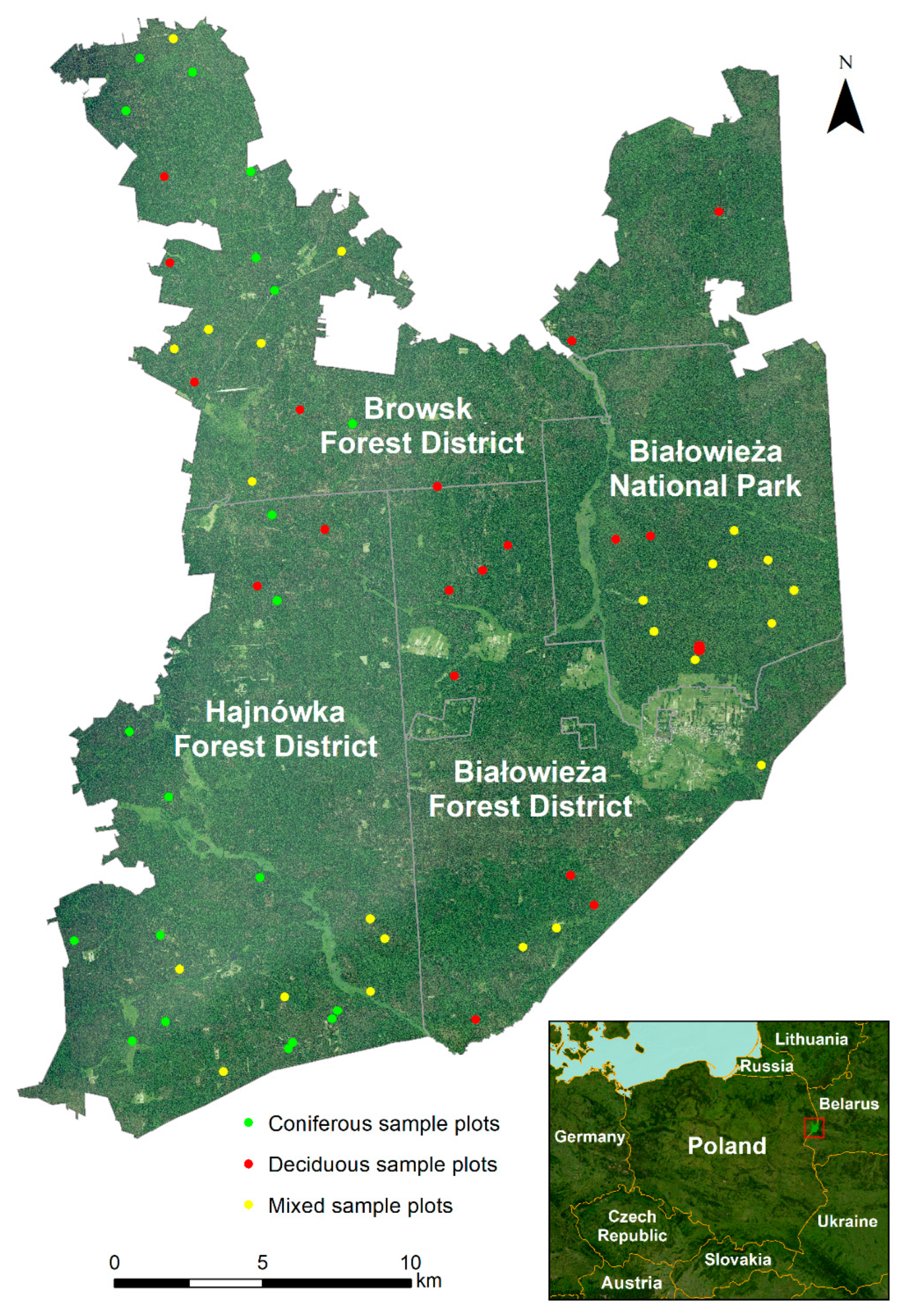
2.1. Study Area

The Białowieża Forest (BF) is an extensive forest area located on the border between Poland and Belarus (52°45′29″N, 23°46′8″E) (Figure 1). Thanks to several years of protection, part of BF has been preserved in close-to-natural forest to this day. The Polish part of BF covers about 62,000 ha, of which 10,500 ha is a Białowieża National Park (BNP); nature reserves cover about 12,000 ha, while the remaining forests are about 39,500 ha. The terrain here is flat with only slight differences in relative elevation (131.6–195.6 m a.s.l.).

The BF area comprises a lowland forest complex characteristic of the Central European ecoregion of mixed forests. The area is of exceptional importance for nature conservation as it includes large intact areas of old-growth forest where natural processes take place. Taking into account the upper layer of the tree stand, the proportion of individual tree species in the BNP is 20%—alder (Alnus glutinosa (L.) Gaertn.); 16%—hornbeam (Carpinus betulus L.); 15%—spruce (Picea abies (L.) H.Karst); 13%—pine (Pinus sylvestris L.); 12%—lime (Tilia cordata Mill.); 9%—oaks (Quercus robur L. and Quercus petraea (Matt.) Liebl.); 6%—birches (Betula pendula Roth., and Betula pubescens Ehrh.); and 9%—others. In turn, in the BF part situated outside the BPN: 23%—spruce; 19%—alder; 17%—pine; 8%—oaks; 8%—hornbeam; 7%—lime; 7%—birches; and 11%—others [39].

2.2. Field Measurement

The field measurements were carried out from July to the end of October 2015. A total of 685 circular sample plots with a radius of 12.62 m were surveyed over the entire area of the Białowieża Forest. The centres of individual plots were accurately measured using a real-time kinematic (RTK) receiver or a static geodetic class receiver for global navigation satellite systems. The SD = 0.096 m was the result of differential pre-processing of the series GNSS data. We assumed similar or better accuracy for the fixed RTK mode, which was used much less frequently due to the dense forest in which the measurements were made. Based on the relationship between the tree and the centre of the sample (distance and azimuth), the position of each tree was calculated. During the field measurement, numerous tree-related characteristics, such as tree species, tree height, diameter at breast height (DBH), crown length and viability of the tree, were collected. In addition, the visibility from above was determined for each tree. In this work, only trees visible from above (i.e., on remote sensing data) were selected to verify the accuracy of the presented correction method.

The verification of the segmentation methods and their corrections was based on a comparative visual assessment between the reference trees and the segments formed during the crown delineation process. For this study, 69 plots with different species diversity, with a total of 1015 trees of nine tree species, were used (

Table 1. Number (n) of reference trees assigned to a particular species. In addition, information on the height range (H_range) and the range of diameter at breast height (DBH_range) is given for each tree species.

Species	n	H_Range (m)	DBH_Range (cm)
Coniferous (20 plots)
Pine	270	16.8–41.0	14.6–75.6
Spruce	131	9.0–44.3	7.5–66.8
Deciduous	21	13.8–32.3	10.9–58.8
Deciduous (26 plots)
Birch	16	20.7–31.1	14.6–36.6
Hornbeam	79	9.1–31.8	8.0–63.0
Lime	55	5.1–34.5	7.6–117
Maple	17	16.8–36.8	13.5–98
Oak	50	17.2–38.7	15.5–117.4
Spruce	20	19.8–37.5	17.9–68.7
Other	14	16.4–34.2	14.9–56.8
Mixed (23 plots)
Alder	55	9.9–36.5	7.4–62.8
Birch	47	9.1–38.0	7.1–66.2
Hornbeam	40	7.9–24.8	7.0–51.0
Lime	10	13.9–28.6	13.3–45.7
Oak	22	17.0–40.2	12.2–111.7
Pine	32	12.1–35.6	15.3–82.2
Poplar	12	21.5–36.7	23–56.1
Spruce	121	8.0–39.0	7.6–71.6
Other	3	18.4–30.6	15.1–50.4

). Furthermore, the plots were divided into three groups based on species composition (forest types):

-

Coniferous—the proportion of spruce and/or pine is over 90%;

-

Deciduous—the proportion of deciduous trees is over 90%;

-

Mixed stands—the proportion of deciduous and coniferous trees is about 50% in each forest type.

2.3. ALS Dataset

The ALS dataset was acquired on 2–5 July 2015 using the LMS-Q680i full waveform system (Riegl, Horn, Austria). The acquired point cloud had an average density of 11 points/m² and its horizontal accuracy was ≤0.20 m, while the vertical accuracy was <0.15 m. The LiDAR strips were overlapped with a coverage of 40% (FOV = 60°). The point cloud was acquired with a maximum scan angle of ±30°. In order to cover the entire study area, 135 individual flight lines were performed. The flight altitude of 500 m resulted in a laser beam footprint of 0.25 m. The data from ALS were used to generate the digital terrain model (DTM) and the digital surface model (DSM) with a resolution of 0.5 m.

The DTM was generated using TerraSolid software (Terrascan, Espoo, Finland), which implements active TIN model algorithm. This filtering method removes non-ground points based on iterative distance and iterative angle [40]. The DSM was generated using the method presented by Erfanifard et al. [41]. To verify the quality of the DTM, 421 ground control points were measured under different conditions (i.e., forests, meadows, public roads). The accuracy of the DTM was expressed by the Root Mean Square Error (RMSE) value of 0.08 m. The models allowed the calculation of a Canopy Height Model (CHM), on the basis of which the segmentation of the individual trees was carried out.

2.4. Segmentation Algorithms

In our work, three automatic segmentation methods were used to identify trees on CHM. Segmentation and subsequent correction were carried out on each of the 69 plots, with the generated CHM in a square buffer of 25 m from the centre of the plot, and then selecting only those segments whose centroid was within the plot boundaries. A brief description of the methods used in the study is presented below.

2.4.1. Local Method

The first method presented is the algorithm described in Stereńczak et al. [27], hereafter referred to as the “Local method”, as it was developed based on the data from the Białowieża Forest area. This method is based on finding local maxima and subsequent extraction of tree crowns by outlining minimum valleys on the CHM with additional segmentation parameterisation in three height ranges (h ≤ 25 m; 25 m < h ≤ 35 m; h > 35 m). For this step, the maximum pixel height value in each segment is used. For each height range, the CHM is filtered with different settings, namely during the automatic optimisation, the kernel size and the sigma value are assigned for each height range. After filtering, a hierarchical segmentation is performed starting from the top layer of the tree canopy using a pouring algorithm [42]. Subsequently, the resulting segments are adjusted using the five-step procedure described in detail in Stereńczak et al. [27].

2.4.2. MCWS 3 × 3 Method

The method presented consists of two steps. In the first step, the method implements a tree detection algorithm based on a local maximum filter to search for potential treetops [43]. The window size can be fixed or variable and the algorithm can work with both raster and point cloud. In this study, we defined the window size as fixed with a kernel size of three pixels. In the second step, the method implements the watershed function [44] to segment (i.e., outline) crowns from a CHM. The segmentation is based on the position of the potential tree crowns determined in an earlier step.

2.4.3. MCWS 5 × 5 Method

The workflow of the method is the same as described in Section 2.4.2. Instead of a kernel size of three pixels, a kernel with a size of five pixels is used for finding the local maxima.

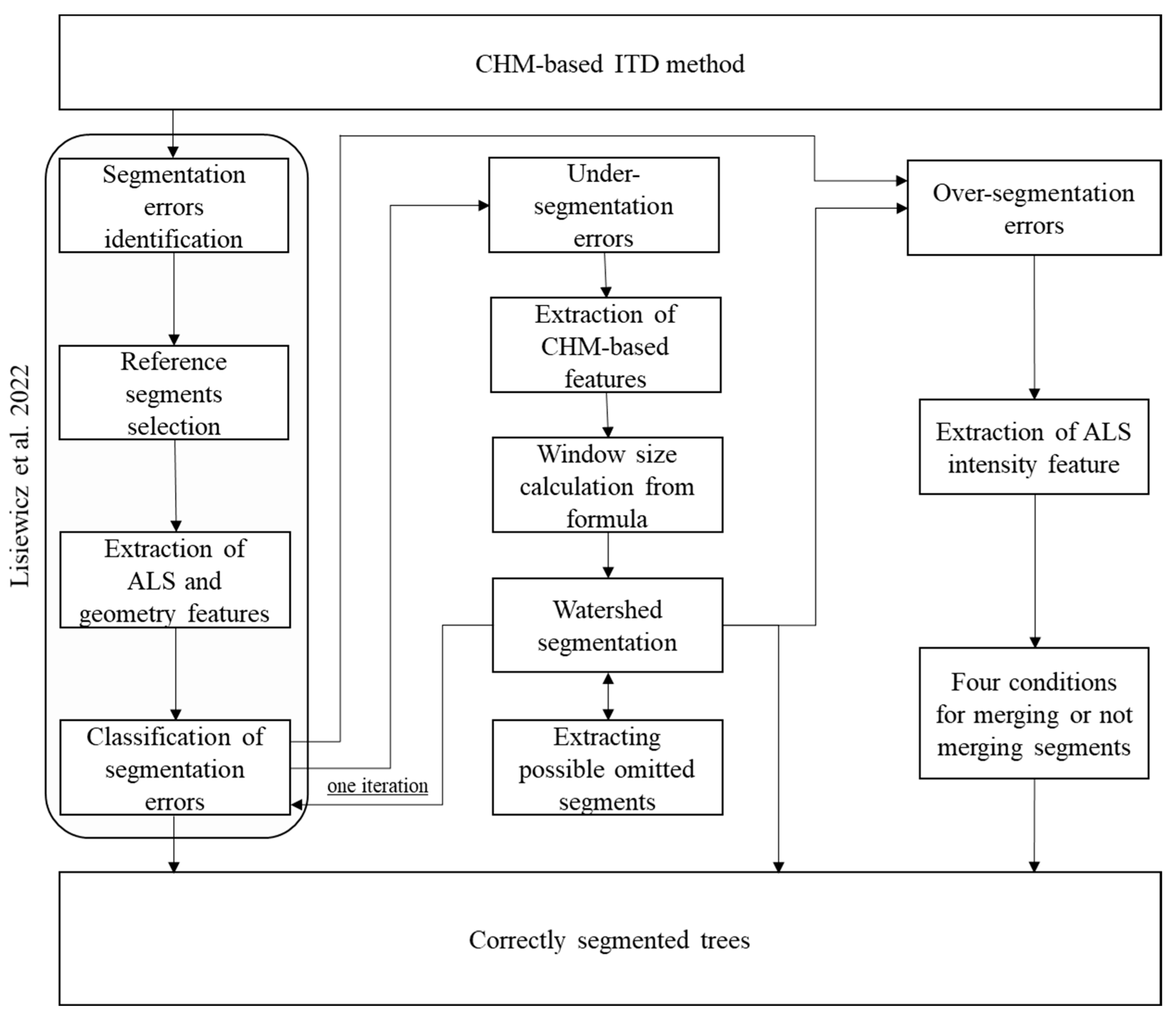
2.5. Correction Method

In this paper, we propose a three-step approach to correct CHM-based individual tree detection errors. In the first step, classification of erroneous (over-segmentation and under-segmentation) and correct segments was performed using the classification method described in Lisiewicz et al. [33]. After classification, the next step was to refine the under-segmentation errors; i.e., to try and separate a segment containing more than one tree. The final step was to merge segments from the over-segmentation class with segments that were classified as correct containing a tree stem, based on the specified conditions.

2.5.1. Recognition and Classification of Segmentation Errors

For the purposes of this paper, we used the method described in Lisiewicz et al. [33] to classify errors in the detection of individual trees. In that study, the authors presented the possibility of distinguishing correct from erroneous segments resulting from CHM-based ITD using the ALS data. Using the Random Forest algorithm and a set of selected predictors from three groups—segment geometry and structural and intensity metrics from the ALS point cloud—it was possible to identify under-segmentation and over-segmentation errors as well as correct segments. High accuracies were obtained for both the training data (OA = 87.0% and κ = 0.794) and test data from 30 sample plots (OA = 85.3% and κ = 0.641). In this study, the classification of segmentation errors was performed for each of the tested and corrected ITD methods. The classification and subsequent correction were performed for segments above 15 m, as the relatively low point cloud density did not allow correct extraction of errors below the 15 m height threshold. Therefore, segments with a height of less than 15 m were automatically assigned to the correct segmentation class. It is worth noting that segments above 15 m height account for about 82% of all segments and 94% of the area of all segments in the BF. Figure 2b shows the classification of the input segments into correct and erroneous classes.

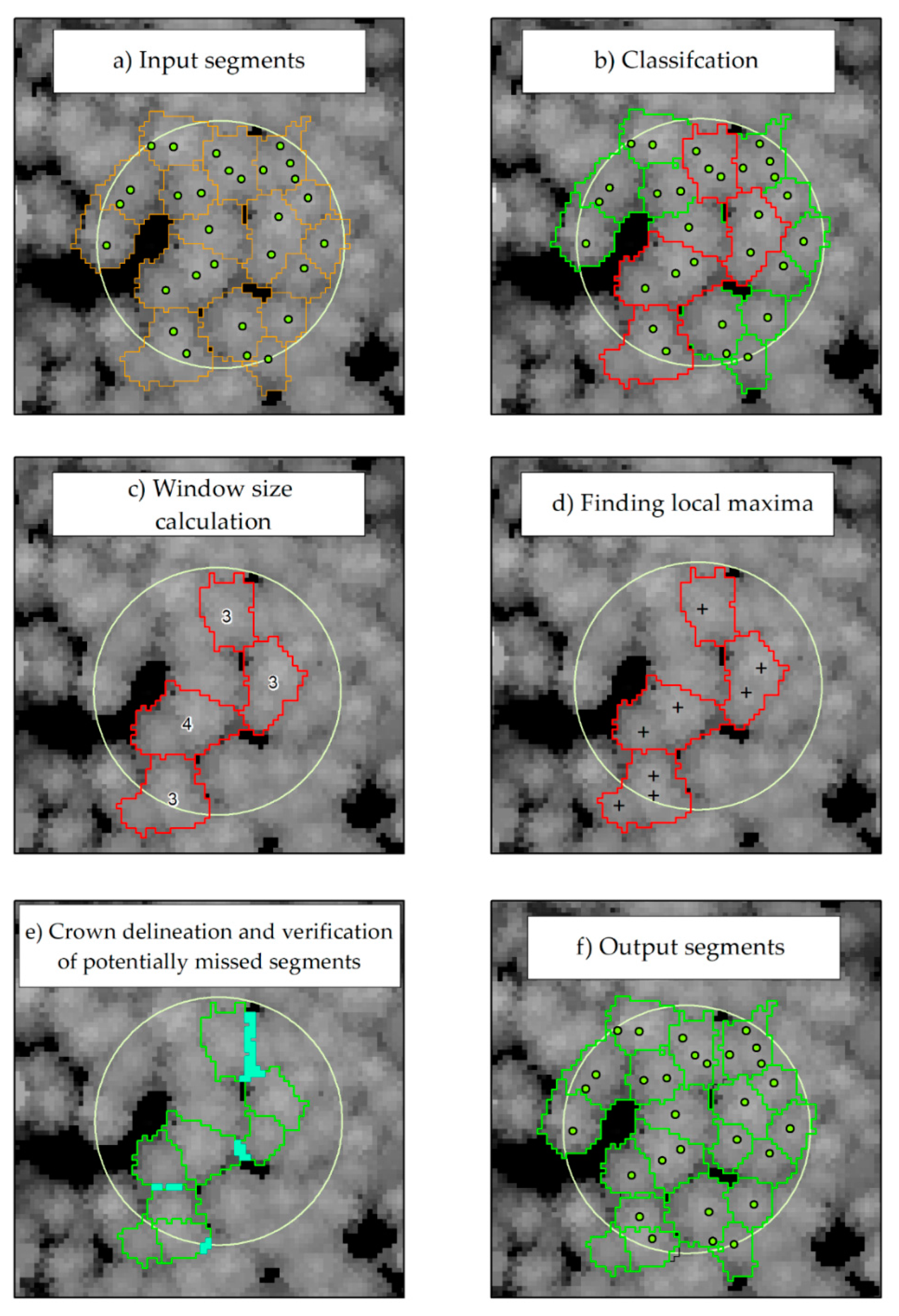
2.5.2. Refine Under-Segmentation Errors

Once the erroneous segments had been extracted during the classification process, segments from the under-segmentation class were selected for further refinement. The correction of the errors in this class consisted of performing a re-segmentation using the method described in Section 2.4.2., based on a defined window size (Figure 2c) to search for local maxima within these segments. The refinement of under-segmentation errors consisted of the following five stages:

(1) The height and volume metrics based on CHM were counted. The different statistics were used to determine their usefulness in the context of determining a window size for re-segmentation. To determine the optimal window size, 131 segments outside the boundaries of the sample plots were selected from the under-segmentation class as a reference. Then, starting with the lowest values, a window size was assigned that would allow correct re-segmentation within the segment. Correct re-segmentation means the correct split of trees in a segment containing two or more trees into separate segments. The first minimum window size value that allows correct re-segmentation was selected. Then, based on a forward stepwise regression, three variables were selected to determine the window size in the search for tree tops, namely, h_median, h_range, and crown_v, where h_median is a median height of CHM overlapping the segment, h_range is the difference between the maximum and minimum height of CHM overlapping the segment, and crown_v is the crown volume calculated from the formula:

$${{\displaystyle \sum }}_{i=1}^{n}re{s}^2\ast \left(h_i-h_{\min }\right)$$

(1)

where:

res—CHM resolution;

h_i—CHM pixel value;

h_min—the minimum height from CHM overlapping the segment;

n—the number of pixels contained in the segment.

The optimal window size (OWS), whose value was rounded to an integer, was calculated from the formula:

$$OWS=1.96+\left(0.00178\ast crow{n}_v\right)+\left(0.06812\ast h_{median}\right)+\left(-0.07653\ast h\_range\right)$$

(2)

R² = 0.70, R²_adj = 0.70, S_e = 0.27

e.g., OWS = 1.96 + (0.00178 × 150) + (0.06812 × 25) + (−0.07653 × 10) = 3.1647 ≈ 3.

(2) Based on the indicated window size, local maxima within the boundaries of the segment with the under-segmentation class were extracted (Figure 2d).

(3) The re-segmentation was performed using the watershed algorithm. Segments whose local maxima were within the input segment were selected. The boundaries of the new segments were restricted to the boundaries of the input segment.

(4) To avoid situations where a tree or a large part of it would not be detected, an additional solution was used to capture such cases. In a complex forest, there were situations where the local maxima were adjacent to the segment boundaries. To extract these cases, the difference between the output and input segments was calculated (Figure 2e). The Classification And Regression Tree method [45] was used to classify the segments to determine whether it is a tree/tree part or not. Considering such cases in the sample plots, 232 reference segments were selected, of which 146 were trees/tree parts and 86 segments that could not be assigned to any tree. The model had an overall accuracy and a kappa coefficient of 97% and 0.94, respectively. Using the CART method, two conditions could be derived based on which segments were selected, namely where:

{Area ∈ <4, 8> and Reock_Score > 0.35} or {Area > 8 and Reock_Score > 0.21}

(3)

where:

Area is the area of the segment;

The Reock Score [46] is the ratio of the area of the segment to the area of the minimum bounding circle of that segment.

(5) The final stage was to reclassify the new segments using the method described in Section 2.5.1. This step was necessary since the algorithm could split a segment from the under-segmentation class into two or more segments, which do not necessarily have to be trees but can also be parts of a tree. For new segments from the under-segmentation class, another iteration was performed, in which the previously mentioned process of segment splitting was carried out again. Subsequently, a re-classification of the segments was carried out. If a segment was again found to be under-segmented, it was assigned to the correct-segmentation class. The output layer of the segments classified as correct and the segments with over-segmentation errors was used for the next correction step, which is described in the following subsection.

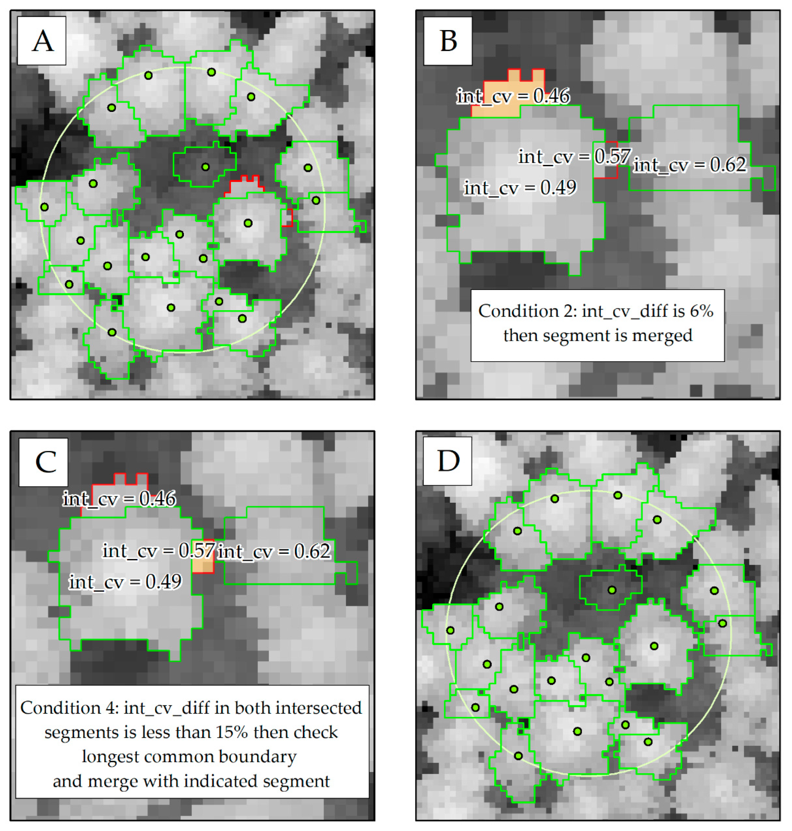
2.5.3. Refine Over-Segmentation Errors

The refinement of the over-segmentation errors consisted of combining segments from this class with segments from the correct-segmentation class (Figure 3A). In a first step, a variety of intensity variables were checked to avoid combining segments from other tree species. Considering the tree species classification in the Białowieża Forest into spruce, pine, deciduous, and dead trees [47], the intensity coefficient of variation (referred to as “int_cv”) variable from the first reflections allowed us to reliably differentiate between these classes. The next step was to set conditions that allowed correct assignment of segments from the over-segmentation class. The following four conditions for the refinement of over-segmentation segments were compiled:

(1) If the segment does not intersect with any other segment, the class has been assigned to the correct-segmentation.

(2) If a segment intersects with only one segment and it is a correct-segmentation class, the int_cv difference between the two segments from the formula was checked:

$$int\_cv\_diff\left(a,b\right)=\frac{\left|int\_cv\left(a\right)-int\_cv\left(b\right)\right|}{\max \left(int\_cv\left(a\right);int\_cv\left(b\right)\right)}\ast 100\%$$

(4)

where:

a, b—the intersecting segments;

int_cv(a), int_cv(b) are the intensity coefficient of variation of the segments of interest.

If $int\_cv\_diff\left(a,b\right)\le 15\%$, the two segments were combined. If $int\_cv\_diff\left(a,b\right)>15\%$, the correct-segmentation class was assigned (Figure 3B).

(3) If a segment intersects with only one segment and it is an over-segmentation class, proceed analogously to condition 2.

(4) If a segment intersects with more than one segment, the following conditions are proposed:

▪

It has been checked how many of them are correct-segmentation. If only one, then the term from condition 2 was executed. If more than one is correct-segmentation and both segments have an int_cv difference of 15% or less, the segment with the longest common boundary was merged (Figure 3C).

▪

In other cases, i.e., if there was more than one segment from the over-segmentation class, the same condition as above was executed.

2.5.4. Segmentation Methods and Correction Validation

A visual method was used to assess the accuracy of individual tree detection by different segmentation methods and their subsequent correction. The visual assessment consisted of comparing the locations of trees from field measurements with the segments generated by the segmentation and correction process. Thanks to the use of high-resolution remote sensing data—georectified images (ground sampling distance (GSD)—0.2 m), CHM (GSD 0.5 m), and ALS point cloud cross-sections (average density of 11 points/m²)—it was possible to accurately assess each segment subjected to segmentation and correction against the tree data measured in the field. Segments with only one equivalent of the field-based measurements were considered to be correctly segmented. Two main segmentation errors were distinguished, namely, over-segmentation (one tree is split into several segments) and under-segmentation (several trees are combined into one segment).

Verification was carried out by two experienced remote sensing specialists who also participated in the field measurements. The verification consisted of assigning to each segment from the output segmentation and correction layers the identifier of the corresponding reference tree from the ground measurements. If a tree was divided into several segments (over-segmentation error), the same reference tree was assigned to each segment. For segments that contained several reference trees, all identifiers were assigned to the segment. No identifiers were assigned to segments that contained no reference trees. If a segment contained a reference tree, but simultaneously also contained a tree outside the sample plot, an additional reference tree was added to the tree reference number.

The evaluation method described by Eysn et al. [19] was used to assess the accuracy of each individual tree detection method and its subsequent correction. The following statistical parameters were calculated for the verification dataset used for the accuracy assessment:

N_Test—Number of extracted trees (segments);

N_Match—Number of reference trees with which a segment matched. If two or more reference trees overlapped with a segment, only one was counted;

N_Ref—Number of reference trees from the top layer of the stand;

N_Com—Number of extracted trees (segments) that could not be matched—N_Com = N_Test − N_Match;

N_Om—Number of reference trees that could not be matched—N_Om = N_Ref − N_Match;

N_Test/N_Ref—Extraction rate;

N_Match/N_Ref—Matching rate;

N_Com/N_Test—Commission rate—test trees that could not be matched;

N_Om/N_Ref—Omission rate—reference trees that could not be matched.

The parameters defined above were used to calculate RMS errors for all plots combined and for selected forest types (coniferous, deciduous, and mixed forest).

RMS_extr—Root mean square of extraction rates;

RMS_ass—Root mean square of matching rates;

RMS_Com—Root mean square of commission rates;

RMS_Om—Root mean square of omission rates.

In addition to the holistic interpretation of the correction results, height subgroups and variations in tree height across the sample plots were also presented. The height subdivision consisted of dividing the sample plots into those where the median tree height was less than 25 m and equal to or more than 25 m. Considering height variability, we subdivided the sample plots in which the coefficient of variation of tree height was less than 15% and equal to or more than 15%.

The complete workflow of the correction method is shown in Figure 4. All processing steps were implemented using a script written in the R language (ver. 4.1.0 [48]) with the following packages: raster [49], rgdal [50], rgeos [51], lidR [52], ForestTools [53], and sf [54].

3. Results

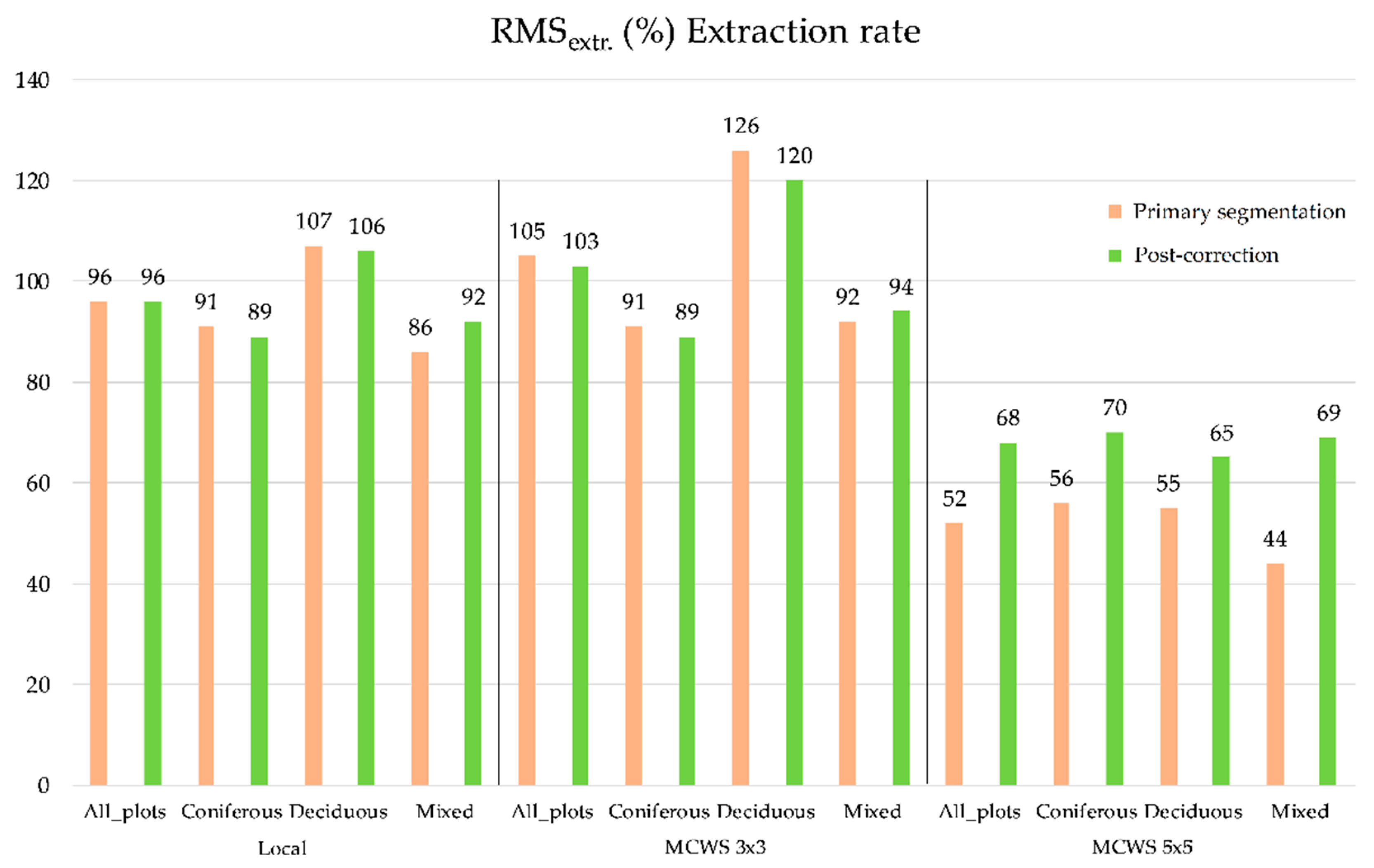
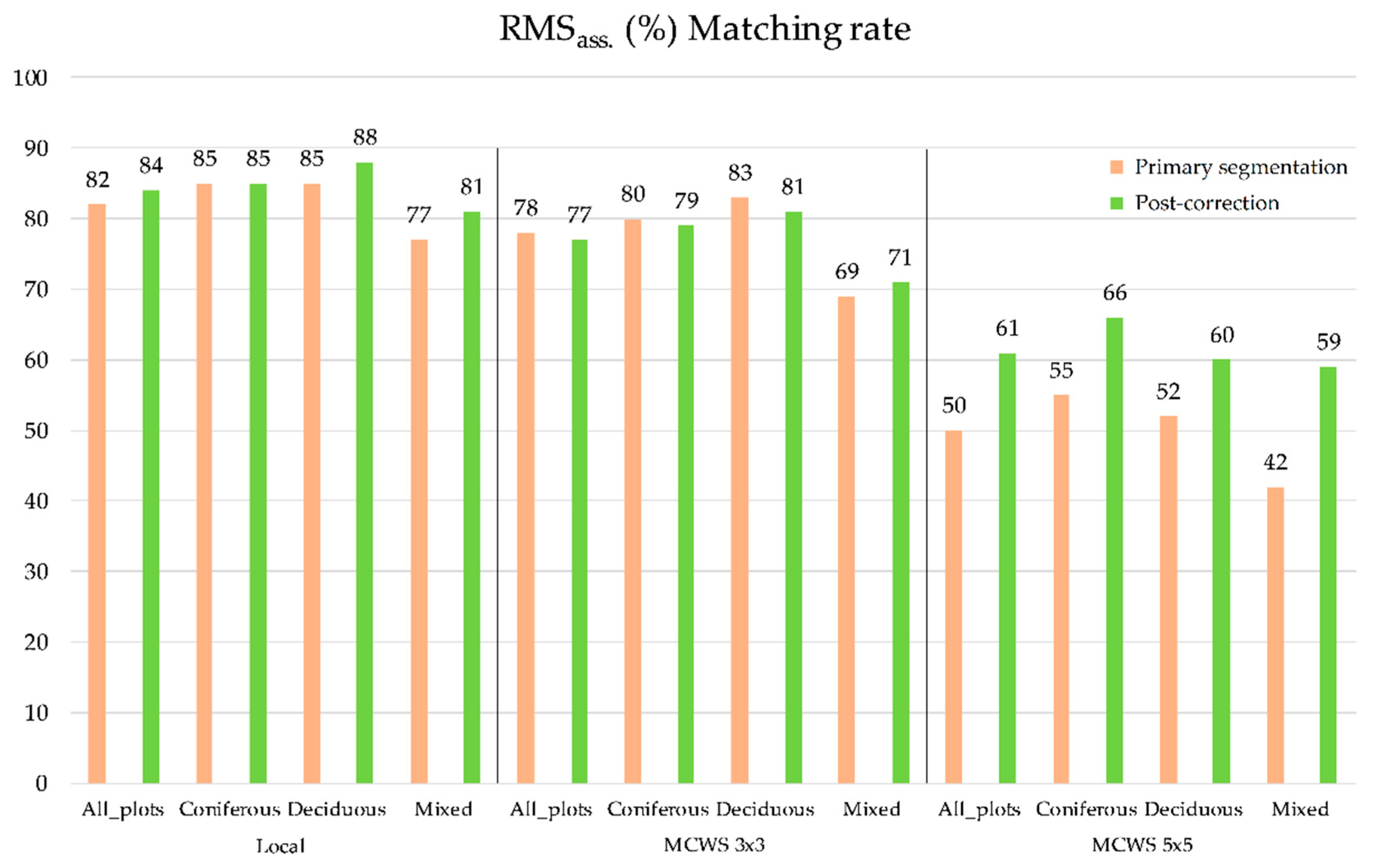
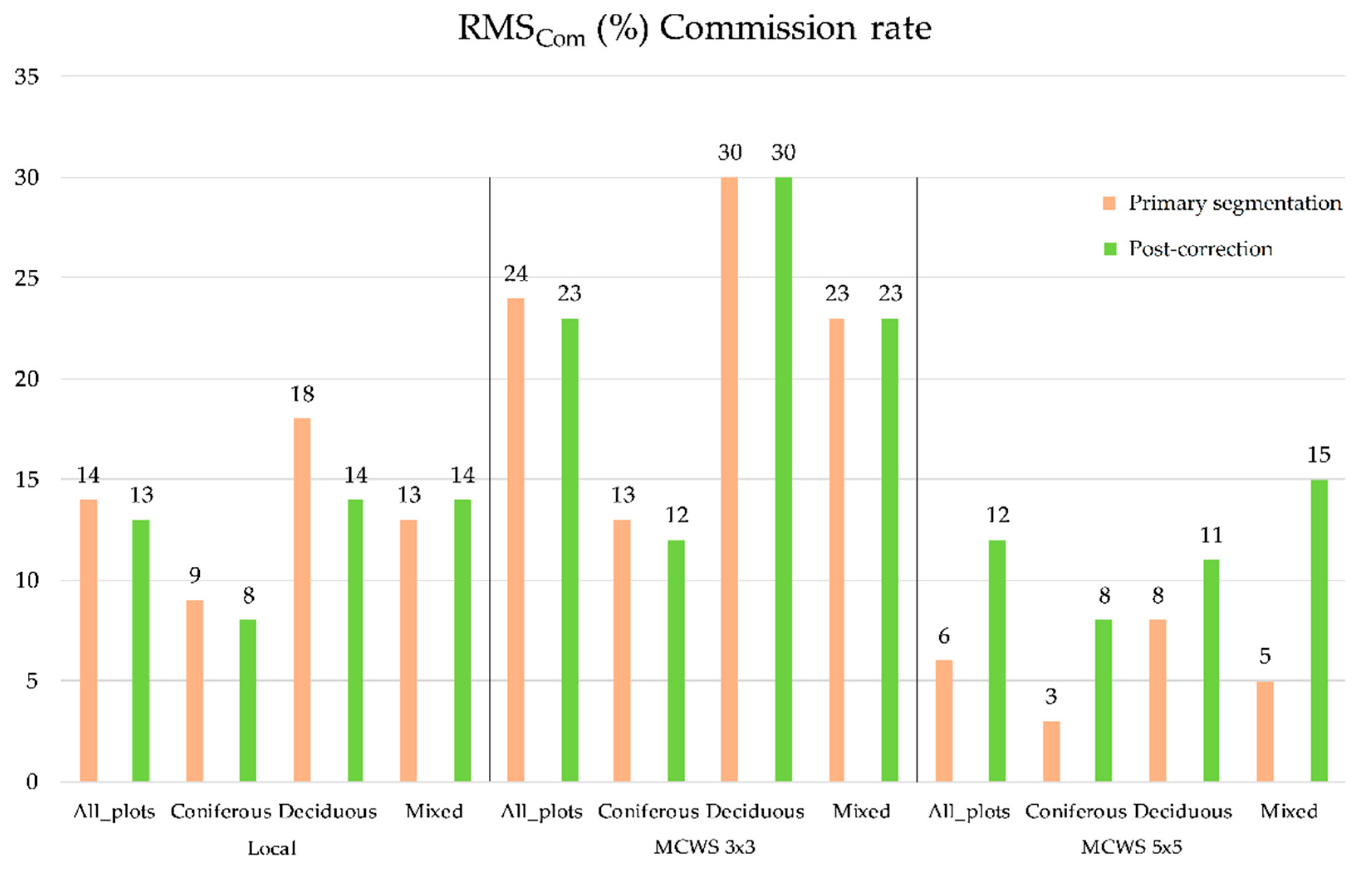
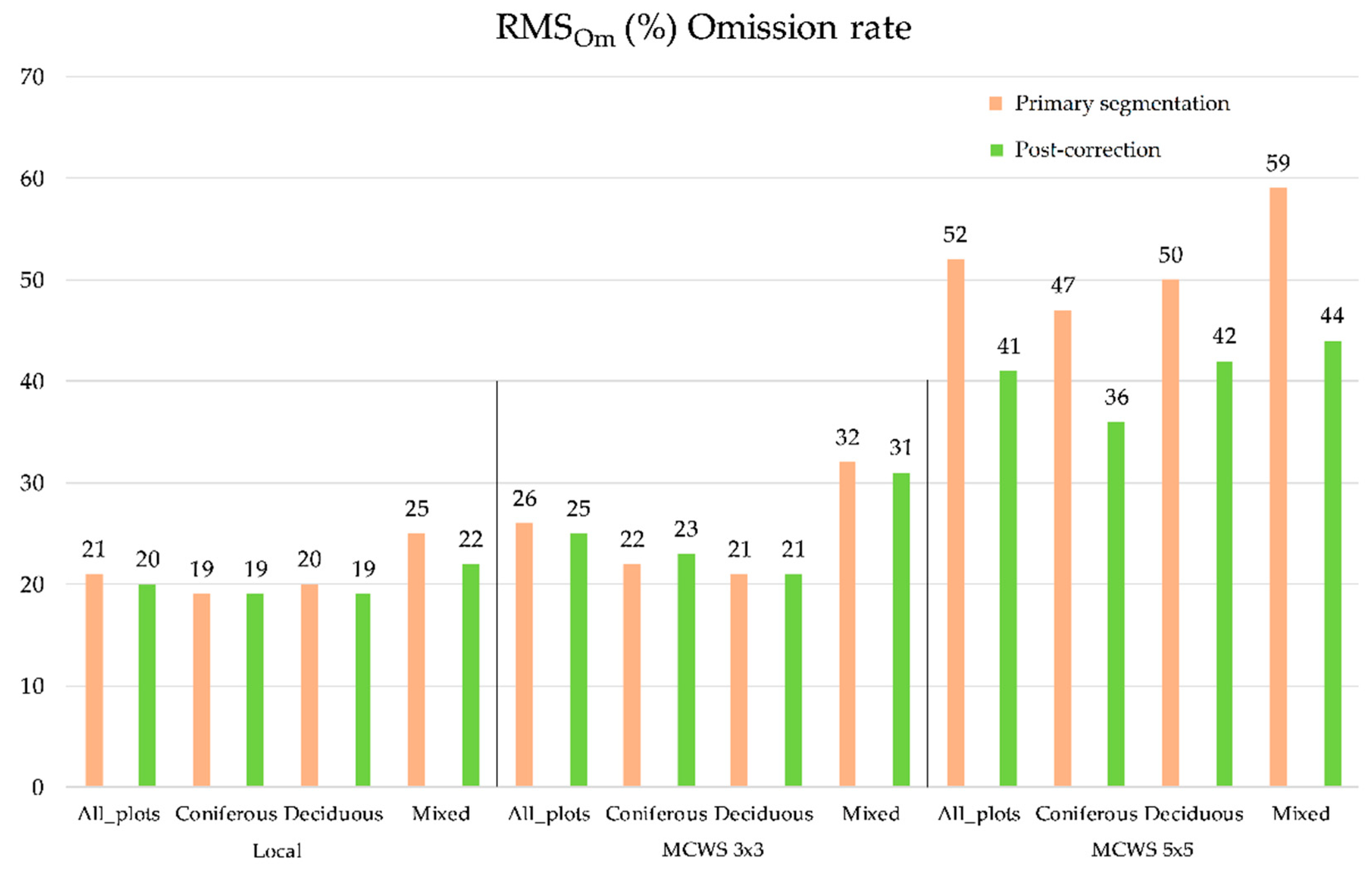
3.1. Overall Matching and Correction Results

Figure 5, Figure 6, Figure 7 and Figure 8 show the summarised detection and correction results for all the tested methods, divided into four groups: all plots, coniferous, deciduous, and mixed plots. The results of the matching, considering different metrics, show how well a method performs for a certain group and what impact the segmentation correction has on this method and group.

The highest extraction rate for all plots (RMS_extr = 105%) was obtained with ‘MCWS 3 × 3′, and the lowest (RMS_extr = 52%) with ‘MCWS 5 × 5′. The correction method improved these results to 103% and 68%, respectively. Looking at the different species groups, the highest extraction rate (RMS_extr = 126%) was found for the deciduous group with ‘MCWS 3 × 3′, and the lowest (RMS_extr = 44%) for the mixed group with ‘MCWS 5 × 5′. The correction method improved these results to 120% and 69%, respectively (Figure 5).

Looking at the matching rates, the highest rate for all plots (RMS_ass. = 82%) was obtained with the ‘Local method’, and the lowest (RMS_ass. = 52%) with ‘MCWS 5 × 5′. The correction method improved these results to 84% and 68%, respectively. Concerning the different species groups, the highest matching rate (RMS_ass. = 85%) was found for the coniferous and deciduous groups with the ‘Local method’, and the lowest (RMS_ass. = 42%) for the mixed group with ‘MCWS 5 × 5′. The correction method improved these results to 88% for the deciduous group with the ‘Local method’ and to 69% for the mixed group with ‘MCWS 5 × 5′ (Figure 6).

Referring to incorrect detections, the highest commission rate for all plots (RMS_Com = 24%) was obtained with ‘MCWS 3 × 3′, and the lowest (RMS_Com = 6%) with ‘MCWS 5 × 5′. The correction method improved results with ‘MCWS 3 × 3′ to 23% and worsened them with ‘MCWS 5 × 5′ to 12%. Looking at the different species groups, the highest commission rate (RMS_Com = 30%) was found for the deciduous group with ‘MCWS 3 × 3′ and the lowest (RMS_Com = 3%) for the coniferous group with ‘MCWS 5 × 5′. The correction method did not improve the results for the deciduous group with ‘MCWS 3 × 3′ (RMS_Com = 30%) and worsened them to 8% for the mixed group with ‘MCWS 5 × 5′ (Figure 7).

The highest omission rate for all plots (RMS_Om), which missed 52% of the indicated reference trees, was obtained with ‘MCWS 5 × 5′. The lowest omission rate (RMS_Om = 21%) was found with the ‘Local method’. The correction method improved these results to 41% and 20%, respectively. For the different species groups, the highest omission rate (RMS_Om = 59%) was found for the mixed group with ‘MCWS 5 × 5′ and the lowest (RMS_Om = 19%) for the coniferous group with ‘Local method’. The correction method improved the results for the mixed group with ‘MCWS 5 × 5′ to 44% and did not improve (RMS_Om = 19%) for the coniferous group with ‘Local method’ (Figure 8).

Looking at all metrics, one can see a significant improvement in the ‘MCWS 5 × 5′ algorithm, where several or more dozen percent improvements were recorded in each metric. Improvements in accuracy were also noted in the ‘Local method’, the most sophisticated of the algorithms used. There was no improvement in results for the ‘MCWS 3 × 3′ method; however, the correction did not affect the tree detection results with this method. It is worth noting that the correction method improved the tree detection results for mixed stands.

3.2. Matching and Correction Results with Various Height Subgroups

To examine the performance of the correction method in detail, the sample plots were divided into those where the median tree height was less than 25 m (

Table 2. Summarised detection and correction results for the subgroup where the median tree height in the sample plot was below 25 m. RMS of the four indicators for all plots is presented. The results for each indicator for the primary segmentation are presented on the left and post-correction on the right.

Method	Group	RMSextr. (%)	RMSass. (%)	RMSCom (%)	RMSOm (%)
		Extraction Rate	Matching Rate	Commission Rate	Omission Rate
Local method	All_plots	86|86	80|80	8|9	22|22
	Coniferous	91|89	85|86	9|5	20|18
	Deciduous	88|87	82|81	9|9	20|21
	Mixed	81|83	76|77	7|10	25|24
MCWS 3 × 3	All_plots	90|92	74|76	18|18	29|27
	Coniferous	81|82	78|80	5|3	22|22
	Deciduous	99|100	79|79	21|21	24|23
	Mixed	78|84	66|70	17|17	35|32
MCWS 5 × 5	All_plots	48|69	47|62	5|12	55|40
	Coniferous	47|71	47|68	0|5	54|33
	Deciduous	51|64	50|61	5|9	52|41
	Mixed	43|74	42|63	5|16	59|39

) and equal to or more than 25 m (

Table 3. Summarised detection and correction results for the subgroup where the median tree height in the sample plot was 25 m or more. RMS of the four indicators for all plots is presented. The results for each indicator for the primary segmentation are presented on the left and post-correction on the right.

Method	Group	RMSextr. (%)	RMSass. (%)	RMSCom (%)	RMSOm (%)
		Extraction Rate	Matching Rate	Commission Rate	Omission Rate
Local method	All_plots	103|104	84|87	17|15	21|19
	Coniferous	91|89	85|84	9|8	19|19
	Deciduous	130|124	86|92	28|20	20|15
	Mixed	90|92	77|81	16|14	24|22
MCWS 3 × 3	All_plots	117|111	80|79	27|26	23|24
	Coniferous	92|90	80|79	14|12	23|23
	Deciduous	163|150	90|85	42|40	14|18
	Mixed	105|104	72|72	28|27	29|30
MCWS 5 × 5	All_plots	53|67	52|61	5|12	51|42
	Coniferous	58|70	57|66	4|8	46|37
	Deciduous	61|67	56|59	11|15	47|43
	Mixed	45|63	43|55	6|14	59|49

). The detailed matching results of the correction according to height subgroups show how well the correction method works under this aspect and considering different forest types.

Considering both height subgroups, the correction results differed for each method. For the ‘Local method’, no improvement was observed in the subgroup below 25 m (same values for extraction and matching rate for all plots). However, in the subgroup for higher trees, an increase in accuracy was observed with a simultaneous decrease in the values for commission and omission rates. This was especially true for the deciduous group, where the extraction and matching rates improved by 6%, while the commission and omission rates improved by 8% and 5%, respectively. The opposite situation occurred for the ‘MCWS 3 × 3′ method, where the correction resulted in improved accuracy for the subgroup below 25 m, especially for the mixed group (increase in extraction and matching rates by 6% and 4%, respectively). In contrast, no significant differences were found for the subgroup equal to or above 25 m, except for the 13% improvement in extraction rate and a concomitant 5% decrease in matching rate in the case of the deciduous group. An analogous situation for this group concerns the commission and omission rates, where the values decreased by 2% and increased by 4%, respectively. For the last method applied, i.e., ‘MCWS 5 × 5′, the correction worked more reliably for the subgroup with smaller trees. Improvement in extraction and matching rates for all plots by 21% and 15%, respectively. A significant improvement in accuracy was observed for the mixed group, extraction and matching rates by 31% and 21%, respectively. There was a 9% increase and a 20% decrease in commission and omission rates, respectively. A similar trend was observed for the taller tree subgroup, but with slightly lower values of improvement; i.e., the extraction and matching rates improved by 14% and 9% for all plots and by 18% and 12% for the mixed group.

3.3. Matching and Correction Results with Various Coefficient of Variation of Height Subgroups

Detailed results were also presented in relation to the variation in height of individual trees in the sample plots, which were divided into those where the coefficient of variation of height (CV_h) was less than 15% (

Table 4. Summarised detection and correction results for the subgroup where the coefficient of variation of tree height in the sample plot was less than 15%. RMS of the four indicators for all plots is presented. The results for each indicator for the primary segmentation are presented on the left and post-correction on the right.

Method	Group	RMSextr. (%)	RMSass. (%)	RMSCom (%)	RMSOm (%)
		Extraction Rate	Matching Rate	Commission Rate	Omission Rate
Local method	All_plots	102|101	84|87	16|13	20|19
	Coniferous	89|88	83|83	9|9	21|20
	Deciduous	117|114	87|93	21|15	18|17
	Mixed	93|102	80|88	17|15	21|17
MCWS 3 × 3	All_plots	116|112	81|80	26|25	22|22
	Coniferous	90|86	80|79	13|11	22|23
	Deciduous	137|129	85|83	33|32	19|20
	Mixed	114|120	75|77	30|31	26|24
MCWS 5 × 5	All_plots	57|70	54|64	6|11	48|37
	Coniferous	57|67	56|64	4|7	47|37
	Deciduous	58|68	55|62	8|11	47|39
	Mixed	52|79	49|67	7|15	52|35

) and equal to or greater than 15% (

Table 5. Summarised detection and correction results for the subgroup where the coefficient of variation of tree height in the sample plot was 15% or more. RMS of the four indicators for all plots is presented. The results for each indicator for the primary segmentation are presented on the left and post-correction on the right.

Method	Group	RMSextr. (%)	RMSass. (%)	RMSCom (%)	RMSOm (%)
		Extraction Rate	Matching Rate	Commission Rate	Omission Rate
Local method	All_plots	86|90	79|81	10|12	23|22
	Coniferous	100|92	94|92	9|0	11|13
	Deciduous	84|90	79|81	9|12	22|22
	Mixed	83|89	75|78	11|13	26|23
MCWS 3 × 3	All_plots	90|92	73|74	20|20	30|29
	Coniferous	91|96	79|83	14|15	23|20
	Deciduous	103|103	80|78	24|25	24|24
	Mixed	82|84	67|68	19|19	34|33
MCWS 5 × 5	All_plots	45|66	44|58	5|13	57|45
	Coniferous	54|79	54|72	0|10	47|32
	Deciduous	49|60	47|55	7|11	55|46
	Mixed	41|64	40|56	5|15	61|47

). The results provide information on how the correction method works in stands with a similar height structure and in stands where the variation in height of individual trees is considerable.

In the first of the methods studied, i.e., the ‘Local method’, considering all plots, the correction improved the results of extraction and matching rates in both subgroups of height variation; in the subgroup below 15% CV_h, by 1% and 3%, respectively, while in the subgroup equal to or above 15% CV_h, by 4% and 2%, respectively. When analysing the individual groups, the greatest improvement was observed with the first subgroup in the mixed group, where the matching rate increased by 8% and the rate of commission and omissions errors decreased by 2% and 4%, respectively. For the second subgroup, the best improvement was also in the mixed group. For the deciduous group, the accuracy of the extraction and matching rates decreased by 6% and 2%, respectively, while the commission rate error increased by 3%. For the ‘MCWS 3 × 3′ method, considering the subgroup with less variation in tree height, there was a 4% increase in the extraction rate with a 1% decrease in the matching rate. In the analysis of the individual groups, the differences in accuracy were small and the differences in commission and omission error rates did not exceed 2% for any of the subgroups. In the subgroup with greater variability in tree height, there was a slight improvement in the extraction and matching rates of 2% and 1%, respectively. The coniferous group improved the most with an increase in extraction and matching rates of 5% and 4%, respectively. However, the deciduous tree group showed lower accuracy as the matching rate decreased by 2%. The differences between the commission and omission rate values were no more than 1% for all groups, except for a 3% improvement in the omission rate in the coniferous group. For the last of the methods used, i.e., ‘MCWS 5 × 5′, an increase in the accuracy of the extraction and matching rates for all plots was observed in both subgroups, by 13% and 10%, respectively, for the subgroup with lower variability, and by 21% and 14%, respectively, for the subgroup with higher variability in tree height. At the same time, commission rate errors increased by 5% and 8% in both subgroups, while the omission rate errors decreased by 11% and 12%, respectively. Looking at the individual groups, the correction in the subgroup with low height variability had the most reliable effect for the mixed group, with an improvement in extraction and matching rates of 13% and 10%, respectively. An analogous situation occurred for the high tree height variability subgroup, where the results of the correction for the mixed group improved the extraction and matching rates by 21% and 16%, respectively.

4. Discussion

In this study, we proposed a three-step approach to refine the segmentation errors arising from CHM-based ITD methods. For this purpose, three methods were tested. In the first step, classification of erroneous (over-segmentation and under-segmentation) and correct segments was performed using the classification method described in Lisiewicz et al. [33]. Using the post-classification layer, the second step was to perform error correction for the under-segmentation class, attempting to extract additional tree crowns within the input segment. The final step was to merge segments from the over-segmentation class with segments classified as correct that contained the tree stem, based on certain conditions. Four indicators were used to show the segmentation accuracy and its subsequent correction. The best correction effects in terms of matching rate were recorded for the mixed plot group, namely, a 4% improvement for the ‘Local method’, 2% for ‘MCWS 3 × 3′, and 17% for ‘MCWS 5 × 5′. Importantly, the study was conducted in one of the most complex and diverse forest communities in Europe, making tree identification a major challenge. Therefore, this study presents a possible solution to reduce segmentation errors by considering different forest types and different ITD methods for identifying individual trees.

4.1. Overall Matching and Correction Results

The correction results differed depending on the method and forest type. The method developed in the study area, i.e., “Local method”, taking into account the matching rate, was improved by 2% when all plots were analysed, and by 3% and 4% when deciduous and mixed plots were considered, respectively. Little or no improvement was expected for coniferous stands, for which the methods were originally developed. This result seems likely, as conifers usually have a clearly defined crown shape. It becomes problematic when treetops and crowns overlap. In this case, under-segmentation errors are difficult to correct. For the ‘MCWS 3 × 3′ method, a 1% decrease was noticed in the matching rate, a 2% improvement in the extraction rate, and a 1% improvement in both the commission and omission rates. The results for this method show that correction did not bring significant changes, except for the mixed group where 1–2% increases in individual accuracy rates were recorded. Mixed stands tend to have higher segmentation errors than homogeneous coniferous stands [34]. It can be explained by mixed forests specificity: diverse species of different heights and crown characteristics are present, in particular in the BF mixed stands. Therefore, classification and subsequent errors correction is more notable in such areas, as these errors actually occur most frequently there. For the ‘MCWS 5 × 5′ method, the improvement taking into account the matching rate and all plots was greatest at 11%, while for the mixed group it was 17%. This method enables for the correct extraction of large trees with spreading crowns but tends to merge crowns of smaller trees; e.g., species such as hornbeam and lime tend to merge crowns due to the lack of distinct treetops and a domed crown structure. Therefore, the commission rate errors were highest for this method. They were corrected by 11% for all plots and 15% for mixed plots.

In other studies, the authors sought suitable solutions to improve their methods and reduce the occurrence of errors as much as possible. Dai et al. [36], in an attempt to avoid under-segmentation errors, classified segments into under-segmentation or non-under-segmentation (correctly detected trees and over-segmentation) with 84% accuracy using the Support Vector Machine method. The authors then refined the segments using the mean-shift ITD method in a common feature space that includes both spatial and multispectral domains. This increased the average tree detection accuracy by 6% and 9% for complex stands. In one of the post-processing steps, Pang et al. [55] treated a tree with a crown diameter greater than half the value of the tree height as an abnormal crown shape, as it is likely to be under-segmented. The corresponding point cloud was then filtered out so that it could be further searched as potential trees in the re-segmentation. Dersch et al. [38] proposed the integration of stem detection with graph-cut segmentation to improve the overall accuracy of the tree segmentation. Considering the F-score, the overall improvement was up to 15% and 6% for reference data from visual interpretation and field measurements, respectively. Our results are difficult to compare due to significant differences in the method used and the density of the point cloud, as a denser point cloud facilitates the extraction of the tree habit. However, dense point clouds are usually collected for small areas, as the processing time for such data is currently too long to apply the solutions for large survey areas. Nevertheless, presently a common trend is to focus on the detection of a tree stem [37,38] or a segment with a tree stem [33] to reliably improve segmentation results.

4.2. Matching and Correction Results with Various Height Subgroups

The vertical structure of the forest seems to have a strong influence on the segmentation results [19]. However, an important aspect is the immediate surroundings of the tree, because in dense stands the crowns of the trees do not always have the crown shape typical for a particular species, as the crowns of neighbouring trees interact with each other, and individual branches interfere with the crowns of neighbouring trees [33]. The results of the correction in the height subgroups varied depending on the segmentation algorithm used. For the ‘Local method’, the correction worked best in the subgroup with high trees, while for the ‘MCWS 3 × 3′ and ‘MCWS 5 × 5′ methods it worked best with small trees. Regardless of subgroup and method, the correction improved segmentation results in mixed stands (except for the subgroup with high trees for ‘MCWS 3 × 3′). When looking at the commission and omission rates, we found that all methods tested and corrected tended to merge the crowns of neighbouring trees (high values for omission rate), possibly due to dense stands where clear boundaries between trees are often missing. The highest commission rates were observed for the ‘MCWS 3 × 3′ method, which uses a small kernel for finding the local maxima and therefore tends to find local irregularities in the CHM, as many such irregularities can be located within individual tree crowns and kernels that are too small tend to detect too many potential trees.

Eysn et al. [19] tested and evaluated eight different segmentation methods, in different study areas, and at different height ranges. Given the identification of small trees, they assumed that small trees in the subdominant layer are theoretically mapped more efficiently at a higher ALS point density. Our study has shown that the accuracy of the segmentation and subsequent correction of small trees also depends on the segmentation method used and the species group analysed. Some studies suggest that tree density, vegetation type and canopy cover affect the results of individual segmentations [56]. Falkowski et al. [57] found that algorithms perform best when canopy cover is less than 50%. Vauhkonen et al. [30] compared various ITD algorithms in different forest types, and their results showed that tree density and clustering are the most important vegetation characteristics affecting segmentation. Considering this, it is extremely important to take into account the characteristics and type of vegetation, as these studies show that their influence on segmentation accuracy is significant. For single species stands, the algorithm is easier to parameterise. This is less the case for mixed stands with several species, as there are additional problems with multiple interactions between neighbouring tree crowns of different species with various heights.

4.3. Matching and Correction Results with Various Coefficient of Variation of Height Subgroups

The accuracy in recognising individual trees is closely related to the immediate environment of the tree being segmented. An important influence on correct segmentation is the height variation of the neighbouring trees. In our study, we used CV _h to divide the sample plots into two subgroups: with low (<0.15) and high (≥ 0.15) tree height variation. Considering the matching rate, lower accuracies were obtained in the plots with the higher height variability. When analysing the correction efficiency, it depended on the specific group and the method used. For the ‘Local method’, correction was more efficient in sample plots with low height variation, improving the accuracy for the deciduous and mixed groups by 6% and 8%, respectively. This shows that the local algorithm took the height differences of the stands into account, among other things, through hierarchical segmentation. For the ‘MCWS 3 × 3′ and ‘MCWS 5 × 5′ methods, the best improvement was for the coniferous group, where CV _h was highest, by 4% and 18%, respectively.

Analogous to our study, other authors have also highlighted the feasibility of characterising forest structure using CV_h. Magnussen et al. [58] suggested that small trees in heterogeneous canopy structures may not be detected because they are obscured by large trees, and therefore the heterogeneous nature of canopy morphology can be characterised by CV_h. Yang et al. [31] also stated that CV_h is a very important feature of vegetation. They claim that a larger CV_h corresponds to more heterogeneous canopy structure and that small trees are more likely to be obscured by large trees, which can significantly reduce the accuracy of tree detection. In mixed forests, the canopies of coniferous and deciduous trees are meaningfully different, which can lead to higher amount of segmentation errors by omission and commission [59,60], as in our study, where most errors occurred in the mixed stands. Apart from the diverse tree species composition of the analysed stands, there is also a huge variation in the mixture of trees—from groups to individual trees, which is an expression of spatial variation. Therefore, algorithm parameterisation is the most difficult when the mixture of tree species and their heights are considerable.

4.4. Outlook

The correction method we have developed can be described as a safe method that attempts to isolate the major errors to refine them. The performance of the method in mixed stands is particularly remarkable. With few exceptions, the correction process does not additionally generate a large number of new errors. However, as with any ITD method, some shortcomings and opportunities for future development are present. Consider-worthy is the acquisition of additional features that would potentially enable correct detection of over-segmentation and under-segmentation errors. Over-segmentation errors, although extracted with high accuracy, can be classified as correct segments in the case of spreading crowns of mature deciduous trees. Under-segmentation errors can be further supported by extracting stems from the point cloud, which is already the case in recent studies. However, one limiting factor is the point cloud density, as in the case of our study. For some species at high scan angles, the stem was not derived from the point cloud, e.g., pine, and the segment was therefore classified as an error. We believe that despite the significant development of point cloud-based methods in the last decade, CHM-based methods in combination with information derived directly from point clouds are worth further development, as the applicability and ease of implementation of CHM-based methods leads to greater capacity and forest management. Therefore, we believe that the correction method developed can significantly improve the ITD results and thus enable a more precise forest analysis; for instance, in the national forest inventories or in the inventory of urban greenery.

5. Conclusions

This study presented a method for correcting segments resulting from CHM-based ITD algorithms. Three ITD methods were tested and corrected in diverse forest stands with different height structures. In a first step, the segmentation errors were classified, and then the under- and over-segmentation errors were refined as efficiently as possible using an automatic correction method. The accuracy of the segmentation improvements varied depending on the method applied and the tree species group studied. The most important findings of the work are as follows:

-

The correction method allows refinement of many segmentation errors.

-

Local ITD methods largely solve many of the potential problems causing errors at the initial stage, so the proposed method is often more effective in improving the results of commonly available methods.

-

In general, the correction method is most efficient for mixed stands, for which the lowest segmentation accuracy is initially obtained. According to the literature, mixed stands have the highest error rate and are the most difficult to parameterise.

-

Using standardised variables for the classification process and refining the over-segmentation errors allows for easier implementation of the method in other study areas without having to adjust the variables.

It is noteworthy that this study was conducted in one of the most complex and diverse forest communities in Europe, which makes tree identification challenging. Therefore, this study offers a possible solution to reduce segmentation errors by considering different forest types and different ITD methods for identifying individual trees.

References

1. Gallo, R.; Grigolato, S.; Cavalli, R.; Mazzetto, F. GNSS-based operational monitoring devices for forest logging operation chains. J. Agric. Eng. 2013, 44. [Google Scholar] [CrossRef]
2. Fardusi, M.J.; Chianucci, F.; Barbati, A. Concept to practices of geospatial information tools to assist forest management & planning under precision forestry framework: A review. Ann. Silvic. Res. 2017, 41, 3–14. [Google Scholar] [CrossRef]
3. Panagiotidis, D.; Abdollahnejad, A.; Slavík, M. Assessment of stem volume on plots using terrestrial laser scanner: A precision forestry application. Sensors 2021, 21, 301. [Google Scholar] [CrossRef] [PubMed]
4. McRoberts, R.E.; Cohen, W.B.; Erik, N.; Stehman, S.V.; Tomppo, E.O. Using remotely sensed data to construct and assess forest attribute maps and related spatial products. Scand. J. For. Res. 2010, 25, 340–367. [Google Scholar] [CrossRef]
5. Dash, J.; Pont, D.; Watt, M.S.; Dash, J.; Pont, D.; Brownlie, R.; Dunningham, A.; Watt, M.S.; Pearse, G. Remote sensing for precision forestry. N. Z. J. For. 2016, 60, 15–24. [Google Scholar]
6. Mielcarek, M.; Kamińska, A.; Stereńczak, K. Digital aerial photogrammetry (DAP) and airborne laser scanning (ALS) as sources of information about tree height: Comparisons of the accuracy of remote sensing methods for tree height estimation. Remote Sens. 2020, 12, 1808. [Google Scholar] [CrossRef]
7. Popescu, S.C.; Wynne, R.H.; Nelson, R.F. Estimating plot-level tree heights with lidar: Local filtering with a canopy-height based variable window size. Comput. Electron. Agric. 2002, 37, 71–95. [Google Scholar] [CrossRef]
8. Błaszczak-Bąk, W.; Janicka, J.; Kozakiewicz, T.; Chudzikiewicz, K.; Bąk, G. Methodology of Calculating the Number of Trees Based on ALS Data for Forestry Applications for the Area of Samławki Forest District. Remote Sens. 2022, 14, 16. [Google Scholar] [CrossRef]
9. Luo, L.; Zhai, Q.; Su, Y.; Ma, Q.; Kelly, M.; Guo, Q. Simple method for direct crown base height estimation of individual conifer trees using airborne LiDAR data. Opt. Express 2018, 26, A562–A578. [Google Scholar] [CrossRef]
10. Korhonen, L.; Vauhkonen, J.; Virolainen, A.; Hovi, A.; Korpela, I. Estimation of tree crown volume from airborne lidar data using computational geometry. Int. J. Remote Sens. 2013, 34, 7236–7248. [Google Scholar] [CrossRef]
11. Lindberg, E.; Hollaus, M. Comparison of Methods for Estimation of Stem Volume, Stem Number and Basal Area from Airborne Laser Scanning Data in a Hemi-Boreal Forest. Remote Sens. 2012, 4, 1004–1023. [Google Scholar] [CrossRef] [Green Version]
12. Yu, X.; Hyyppä, J.; Vastaranta, M.; Holopainen, M.; Viitala, R. Predicting individual tree attributes from airborne laser point clouds based on the random forests technique. ISPRS J. Photogramm. Remote Sens. 2011, 66, 28–37. [Google Scholar] [CrossRef]
13. Magdon, P.; González-Ferreiro, E.; Pérez-Cruzado, C.; Purnama, E.S.; Sarodja, D.; Kleinn, C. Evaluating the Potential of ALS Data to Increase the Efficiency of Aboveground Biomass Estimates in Tropical Peat–Swamp Forests. Remote Sens. 2018, 10, 1344. [Google Scholar] [CrossRef] [Green Version]
14. Koch, B.; Heyder, U.; Welnacker, H. Detection of individual tree crowns in airborne lidar data. Photogramm. Eng. Remote. Sens. 2006, 72, 357–363. [Google Scholar] [CrossRef] [Green Version]
15. Zhen, Z.; Quackenbush, L.J.; Zhang, L. Trends in automatic individual tree crown detection and delineation-evolution of LiDAR data. Remote Sens. 2016, 8, 333. [Google Scholar] [CrossRef] [Green Version]
16. Koch, B.; Kattenborn, T.; Straub, C.; Vauhkonen, J. Segmentation of forest to tree objects. In Forestry Applications of Airborne Laser Scanning: Concepts and Case Studies; Maltamo, M., Næsset, E., Vauhkonen, J., Eds.; Springer: Dordrecht, The Netherlands, 2014; pp. 89–112. ISBN 978-94-017-8663-8. [Google Scholar]
17. Shamsoddini, A.; Turner, R.; Trinder, J.C. Improving lidar-based forest structure mapping with crown-level pit removal. J. Spat. Sci. 2013, 58, 29–51. [Google Scholar] [CrossRef]
18. Zhao, D.; Pang, Y.; Li, Z.; Sun, G. Filling invalid values in a lidar-derived canopy height model with morphological crown control. Int. J. Remote Sens. 2013, 34, 4636–4654. [Google Scholar] [CrossRef]
19. Eysn, L.; Hollaus, M.; Lindberg, E.; Berger, F.; Monnet, J.M.; Dalponte, M.; Kobal, M.; Pellegrini, M.; Lingua, E.; Mongus, D.; et al. A benchmark of lidar-based single tree detection methods using heterogeneous forest data from the Alpine Space. Forests 2015, 6, 1721–1747. [Google Scholar] [CrossRef] [Green Version]
20. Wang, Y.; Hyyppa, J.; Liang, X.; Kaartinen, H.; Yu, X.; Lindberg, E.; Holmgren, J.; Qin, Y.; Mallet, C.; Ferraz, A.; et al. International Benchmarking of the Individual Tree Detection Methods for Modeling 3-D Canopy Structure for Silviculture and Forest Ecology Using Airborne Laser Scanning. IEEE Trans. Geosci. Remote Sens. 2016, 54, 5011–5027. [Google Scholar] [CrossRef] [Green Version]
21. Stereńczak, K. Factors influencing individual tree crowns detection based on airborne laser scanning data. For. Res. Pap. 2013, 74, 323–333. [Google Scholar] [CrossRef] [Green Version]
22. Hyyppä, J.; Kelle, O.; Lehikoinen, M.; Inkinen, M. A segmentation-based method to retrieve stem volume estimates from 3-D tree height models produced by laser scanners. IEEE Trans. Geosci. Remote Sens. 2001, 39, 969–975. [Google Scholar] [CrossRef]
23. Persson, Å.; Holmgren, J.; Söderman, U. Detecting and measuring individual trees using an airborne laser scanner. Photogramm. Eng. Remote. Sens. 2002, 68, 925–932. [Google Scholar]
24. Hyyppä, J.; Inkinen, M. Detecting and estimating attribute for single trees using laser scanner. Photogramnetric J. Finl. 1999, 16, 27–42. [Google Scholar]
25. Larsen, M.; Eriksson, M.; Descombes, X.; Perrin, G.; Brandtberg, T.; Gougeon, F.A. Comparison of six individual tree crown detection algorithms evaluated under varying forest conditions. Int. J. Remote Sens. 2011, 32, 5827–5852. [Google Scholar] [CrossRef]
26. Wang, X.H.; Zhang, Y.Z.; Xu, M.M. A multi-threshold segmentation for tree-level parameter extraction in a deciduous forest using small-footprint airborne LiDAR data. Remote Sens. 2019, 11, 2109. [Google Scholar] [CrossRef] [Green Version]
27. Stereńczak, K.; Kraszewski, B.; Mielcarek, M.; Piasecka, Ż.; Lisiewicz, M.; Heurich, M. Mapping individual trees with airborne laser scanning data in an European lowland forest using a self-calibration algorithm. Int. J. Appl. Earth Obs. Geoinf. 2020, 93, 102191. [Google Scholar] [CrossRef]
28. Jing, L.; Hu, B.; Li, J.; Noland, T. Automated delineation of individual tree crowns from lidar data by multi-scale analysis and segmentation. Photogramm. Eng. Remote. Sens. 2012, 78, 1275–1284. [Google Scholar] [CrossRef]
29. Hamraz, H.; Contreras, M.A.; Zhang, J. A robust approach for tree segmentation in deciduous forests using small-footprint airborne LiDAR data. Int. J. Appl. Earth Obs. Geoinf. 2016, 52, 532–541. [Google Scholar] [CrossRef] [Green Version]
30. Vauhkonen, J.; Ene, L.; Gupta, S.; Heinzel, J.; Holmgren, J.; Pitkänen, J.; Solberg, S.; Wang, Y.; Weinacker, H.; Hauglin, K.M.; et al. Comparative testing of single-tree detection algorithms under different types of forest. Forestry 2012, 85, 27–40. [Google Scholar] [CrossRef] [Green Version]
31. Yang, Q.; Su, Y.; Jin, S.; Kelly, M.; Hu, T.; Ma, Q.; Li, Y.; Song, S.; Zhang, J.; Xu, G.; et al. The influence of vegetation characteristics on individual tree segmentation methods with airborne LiDAR data. Remote Sens. 2019, 11, 2880. [Google Scholar] [CrossRef] [Green Version]
32. Hastings, J.H.; Ollinger, S.V.; Ouimette, A.P.; Sanders-DeMott, R.; Palace, M.W.; Ducey, M.J.; Sullivan, F.B.; Basler, D.; Orwig, D.A. Tree Species Traits Determine the Success of LiDAR-Based Crown Mapping in a Mixed Temperate Forest. Remote Sens. 2020, 12, 309. [Google Scholar] [CrossRef] [Green Version]
33. Lisiewicz, M.; Kamińska, A.; Stereńczak, K. Recognition of specified errors of Individual Tree Detection methods based on Canopy Height Model. Remote Sens. Appl. Soc. Environ. 2022, 25, 100690. [Google Scholar] [CrossRef]
34. Kankare, V.; Räty, M.; Yu, X.; Holopainen, M.; Vastaranta, M.; Kantola, T.; Hyyppä, J.; Hyyppä, H.; Alho, P.; Viitala, R. Single tree biomass modelling using airborne laser scanning. ISPRS J. Photogramm. Remote Sens. 2013, 85, 66–73. [Google Scholar] [CrossRef]
35. Wolf, B.M.; Heipke, C. Automatic extraction and delineation of single trees from remote sensing data. Mach. Vis. Appl. 2007, 18, 317–330. [Google Scholar] [CrossRef]
36. Dai, W.; Yang, B.; Dong, Z.; Shaker, A. A new method for 3D individual tree extraction using multispectral airborne LiDAR point clouds. ISPRS J. Photogramm. Remote Sens. 2018, 144, 400–411. [Google Scholar] [CrossRef]
37. Wang, X.; Zhang, Y.; Luo, Z. Combining Trunk Detection with Canopy Segmentation to Delineate Single Deciduous Trees Using Airborne LiDAR Data. IEEE Access 2020, 8, 99783–99796. [Google Scholar] [CrossRef]
38. Dersch, S.; Heurich, M.; Krueger, N.; Krzystek, P. Combining graph-cut clustering with object-based stem detection for tree segmentation in highly dense airborne lidar point clouds. ISPRS J. Photogramm. Remote Sens. 2021, 172, 207–222. [Google Scholar] [CrossRef]
39. Stereńczak, K.; Kraszewski, B.; Mielcarek, M.; Kamińska, A.; Lisiewicz, M.; Modzelewska, A.; Sadkowski, R.; Białczak, M.; Piasecka, Ż.; Wilkowska, R. The Białowieża Forest monitoring with the use of remote sensing data. In Zimowa Szkoła Leśna XI Sesja-Zastosowanie Geoinformatyki w Leśnictwie; Instytut Badawczy Leśnictwa: Sękocin Stary, Poland, 2020; pp. 99–107. (In Polish) [Google Scholar]
40. Axelsson, P. DEM generation from laser scanner data using adaptive TIN models. Int. Arch. Photogramm. Remote Sens. 2000, 33, 110–117. [Google Scholar]
41. Erfanifard, Y.; Stereńczak, K.; Kraszewski, B.; Kamińska, A. Development of a robust canopy height model derived from ALS point clouds for predicting individual crown attributes at the species level. Int. J. Remote Sens. 2018, 39, 9206–9227. [Google Scholar] [CrossRef]
42. Soille, P. Morphological Image Analysis: Principles and Applications; Springer: Berlin/Heidelberg, Germany, 1999; ISBN 978-3-662-03941-0. [Google Scholar]
43. Popescu, S.C.; Wynne, R.H. Seeing the Trees in the Forest: Using Lidar and Multispectral Data Fusion with Local Filtering and Variable Window Size for Estimating Tree Height. Photogramm. Eng. Remote Sens. 2004, 70, 589–604. [Google Scholar] [CrossRef] [Green Version]
44. Meyer, F.; Beucher, S. Morphological segmentation. J. Vis. Commun. Image Represent. 1990, 1, 21–46. [Google Scholar] [CrossRef]
45. Breiman, L.; Friedman, J.H.; Olshen, R.A.; Stone, C.J. Classification and Regression Trees, 1st ed.; Routledge: Boca Raton, FL, USA, 1984. [Google Scholar]
46. Reock, E.C. A Note: Measuring Compactness as a Requirement of Legislative Apportionment. Midwest J. Polit. Sci. 1961, 5, 70–74. [Google Scholar] [CrossRef]
47. Kamińska, A.; Lisiewicz, M.; Stereńczak, K.; Kraszewski, B.; Sadkowski, R. Species-related single dead tree detection using multi-temporal ALS data and CIR imagery. Remote Sens. Environ. 2018, 219, 31–43. [Google Scholar] [CrossRef]
48. R Foundation for Statistical Computing. R Development Core Team R: A Language and Environment for Statistical Computing; R Foundation for Statistical Computing: Vienna, Austria, 2021; Available online: https://www.r-project.org/ (accessed on 20 February 2022).
49. Hijmans, R.J. Raster: Geographic Data Analysis and Modeling; Version 3.5-15; R Core Team: Vienna, Austria, 2022. [Google Scholar]
50. Bivand, R.; Keitt, T.; Rowlingson, B. Rgdal: Bindings for the “Geospatial” Data Abstraction Library; Version 1.5-29; R Core Team: Vienna, Austria, 2022. [Google Scholar]
51. Bivand, R.; Rundel, C. Rgeos: Interface to Geometry Engine-Open Source (‘GEOS’) Version 0.5-9; R Core Team: Vienna, Austria, 2021. [Google Scholar]
52. Roussel, J.R.; Auty, D.; Coops, N.C.; Tompalski, P.; Goodbody, T.R.H.; Meador, A.S.; Bourdon, J.F.; de Boissieu, F.; Achim, A. lidR: An R package for analysis of Airborne Laser Scanning (ALS) data. Remote Sens. Environ. 2020, 251, 112061. [Google Scholar] [CrossRef]
53. Plowright, A.; Roussel, J.R. ForestTools: Analyzing Remotely Sensed Forest Data; Version 0.2.5; R Core Team: Vienna, Austria, 2021. [Google Scholar]
54. Pebesma, E. Simple Features for R: Standardized Support for Spatial Vector Data. R J. 2018, 10, 439–446. [Google Scholar] [CrossRef] [Green Version]
55. Pang, Y.; Wang, W.; Du, L.; Zhang, Z.; Liang, X.; Li, Y.; Wang, Z. Nyström-based spectral clustering using airborne LiDAR point cloud data for individual tree segmentation. Int. J. Digit. Earth 2021, 14, 1452–1476. [Google Scholar] [CrossRef]
56. Peuhkurinen, J.; Mehtätalo, L.; Maltamo, M. Comparing individual tree detection and the areabased statistical approach for the retrieval of forest stand characteristics using airborne laser scanning in Scots pine stands. Can. J. For. Res. 2011, 41, 583–598. [Google Scholar] [CrossRef]
57. Falkowski, M.J.; Smith, A.M.S.; Gessler, P.E.; Hudak, A.T.; Vierling, L.A.; Evans, J.S. The influence of conifer forest canopy cover on the accuracy of two individual tree measurement algorithms using lidar data. Can. J. Remote Sens. 2008, 34, 338–350. [Google Scholar] [CrossRef]
58. Magnussen, S.; Eggermont, P.; LaRiccia, V.N. Recovering Tree Heights from Airborne Laser Scanner Data. For. Sci. 1999, 45, 407–422. [Google Scholar] [CrossRef]
59. Forzieri, G.; Guarnieri, L.; Vivoni, E.R.; Castelli, F.; Preti, F. Multiple attribute decision making for individual tree detection using high-resolution laser scanning. For. Ecol. Manag. 2009, 258, 2501–2510. [Google Scholar] [CrossRef]
60. Jakubowski, M.; Li, W.; Guo, Q.; Kelly, M. Delineating Individual Trees from Lidar Data: A Comparison of Vector- and Raster-based Segmentation Approaches. Remote Sens. 2013, 5, 4163–4186. [Google Scholar] [CrossRef] [Green Version]
Figure 1. Polish part of the Białowieża Forest with the selected sample plots.
Remotesensing 14 01822 g001
Figure 2. Graphical scheme for refining under-segmentation errors on one of the sample plots. The orange boundaries indicate the extent of the segments of ITD, while the green and red boundaries indicate classification to correct and erroneous classes, respectively. Green dots indicate trees measured in the field, while “+” indicates the local maxima found. Segments highlighted in blue indicate potentially missed segments.
Remotesensing 14 01822 g002
Figure 3. Graphical scheme for refining over-segmentation errors on one of the sample plots. (A) Input segments after under-segmentation refinement; (B) highlighted segment correction in accordance with condition 2; (C) highlighted segment correction in accordance with condition 4; (D) output segments.
Remotesensing 14 01822 g003
Figure 4. Workflow of the proposed method for correcting segmentation errors.
Remotesensing 14 01822 g004
Figure 5. Bar chart for the extraction rate for the different segmentation methods and species groups.
Remotesensing 14 01822 g005
Figure 6. Bar chart for the matching rate for the different segmentation methods and species groups.
Remotesensing 14 01822 g006
Figure 7. Bar chart for the commission rate for the different segmentation methods and species groups.
Remotesensing 14 01822 g007
Figure 8. Bar chart for the omission rate for the different segmentation methods and species groups.
Remotesensing 14 01822 g008