
Surface Current Variations and Hydrological Characteristics of the Penghu Channel in the Southeastern Taiwan Strait


Abstract
1. Introduction
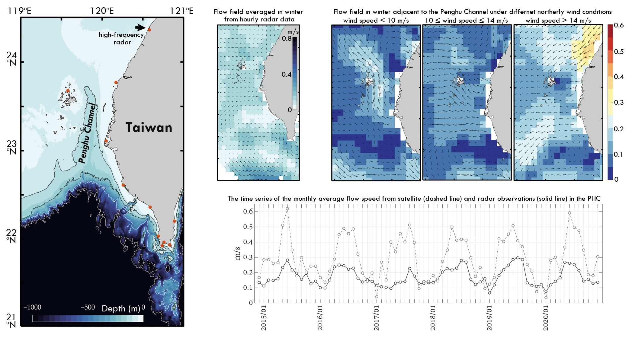
2. Data
2.1. Ocean Currents
2.1.1. Satellite Observations
2.1.2. Survey Observations
2.1.3. SeaSonde HF Radar Observations
2.2. In Situ Observations
2.2.1. Surface Drifter
2.2.2. Historical Hydrological Observations
2.3. Temperature, Salinity, Chlorophyll Concentration, and Wind
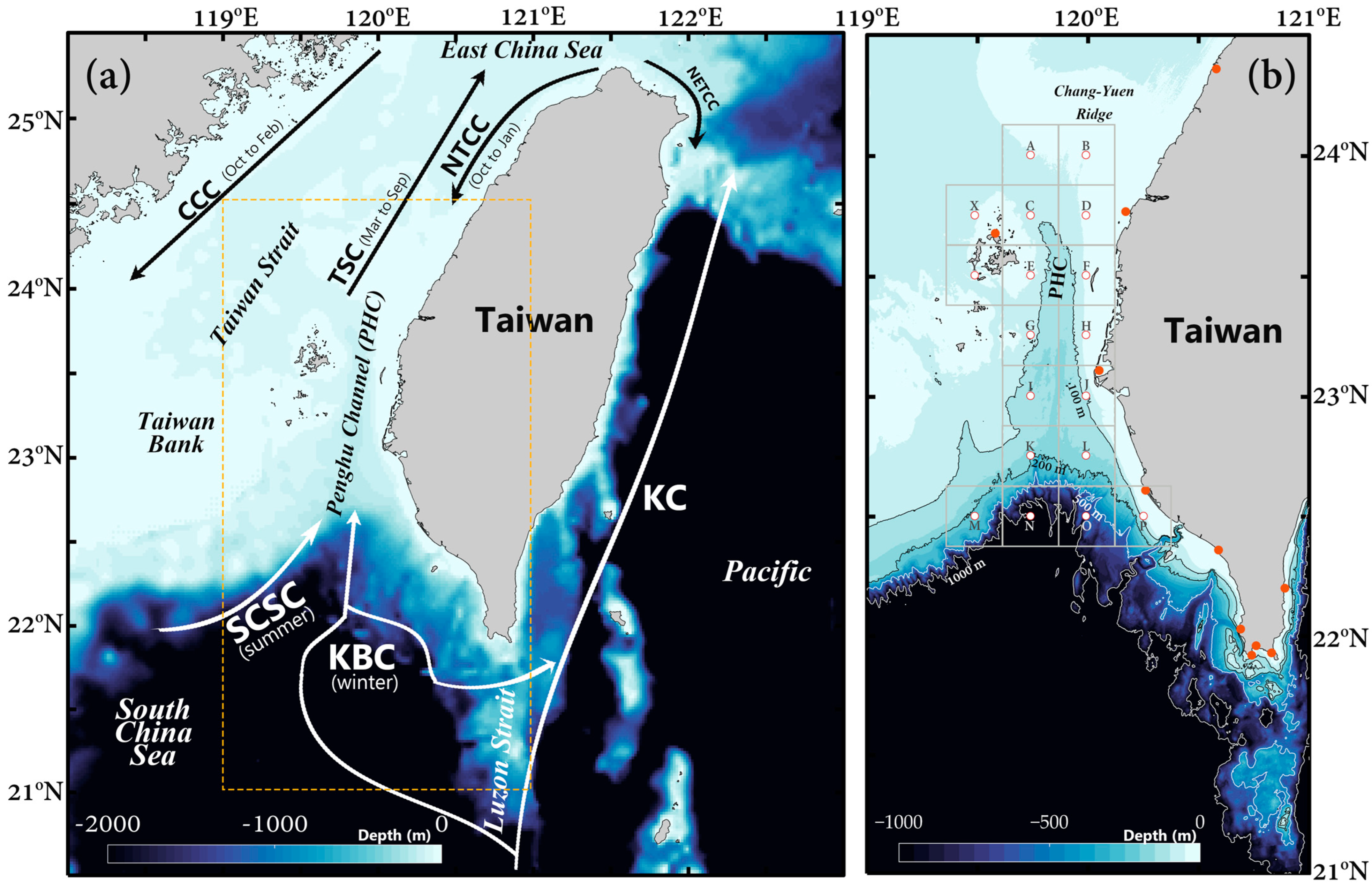
3. Ocean Currents Adjacent to the PHC
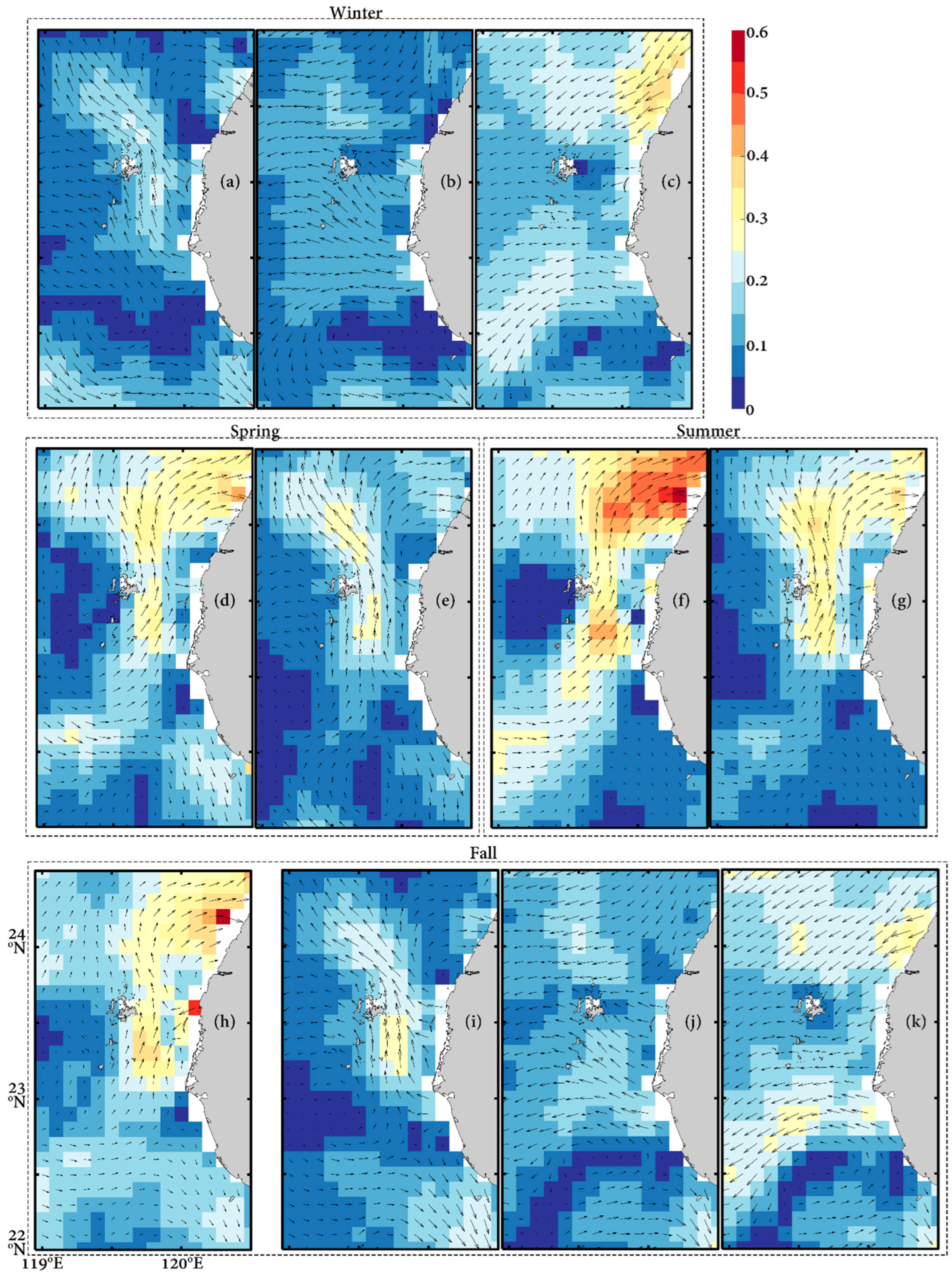
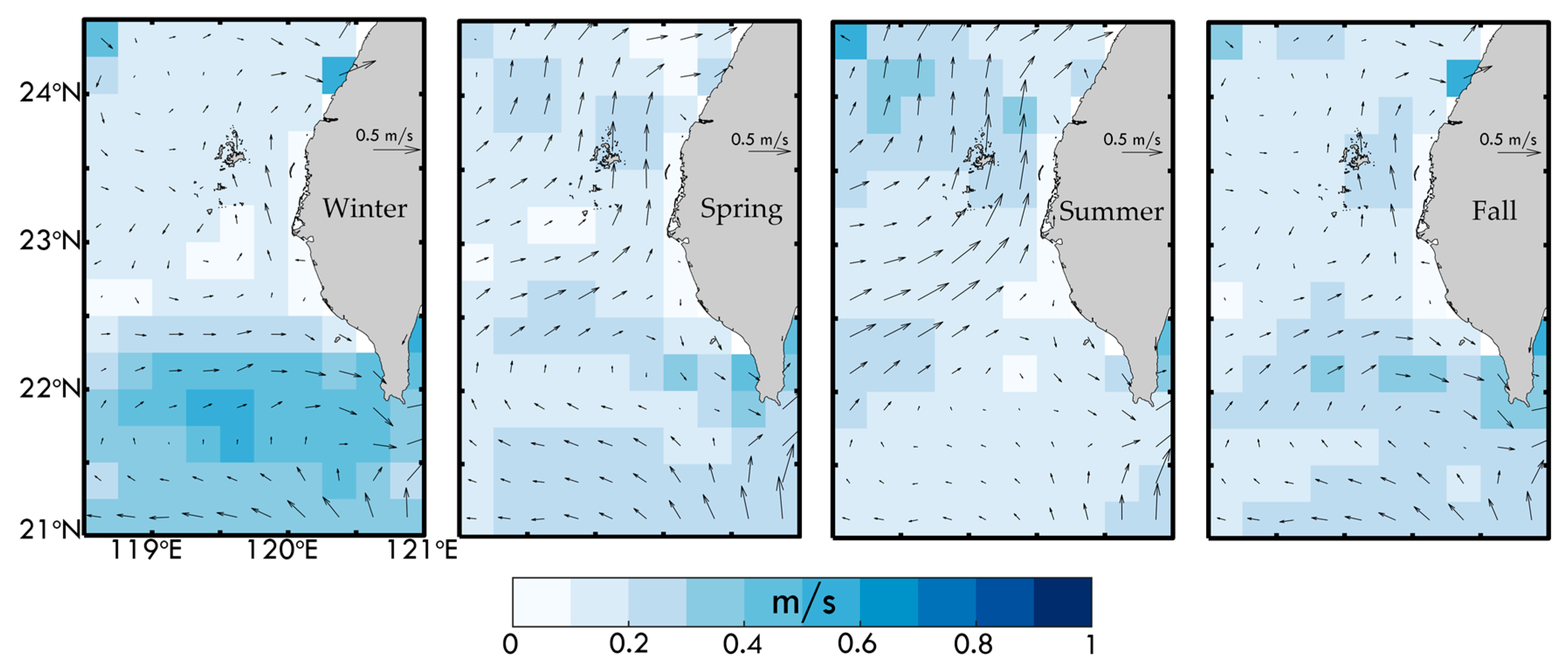
3.1. Satellite Observation and Historical Survey Measurements
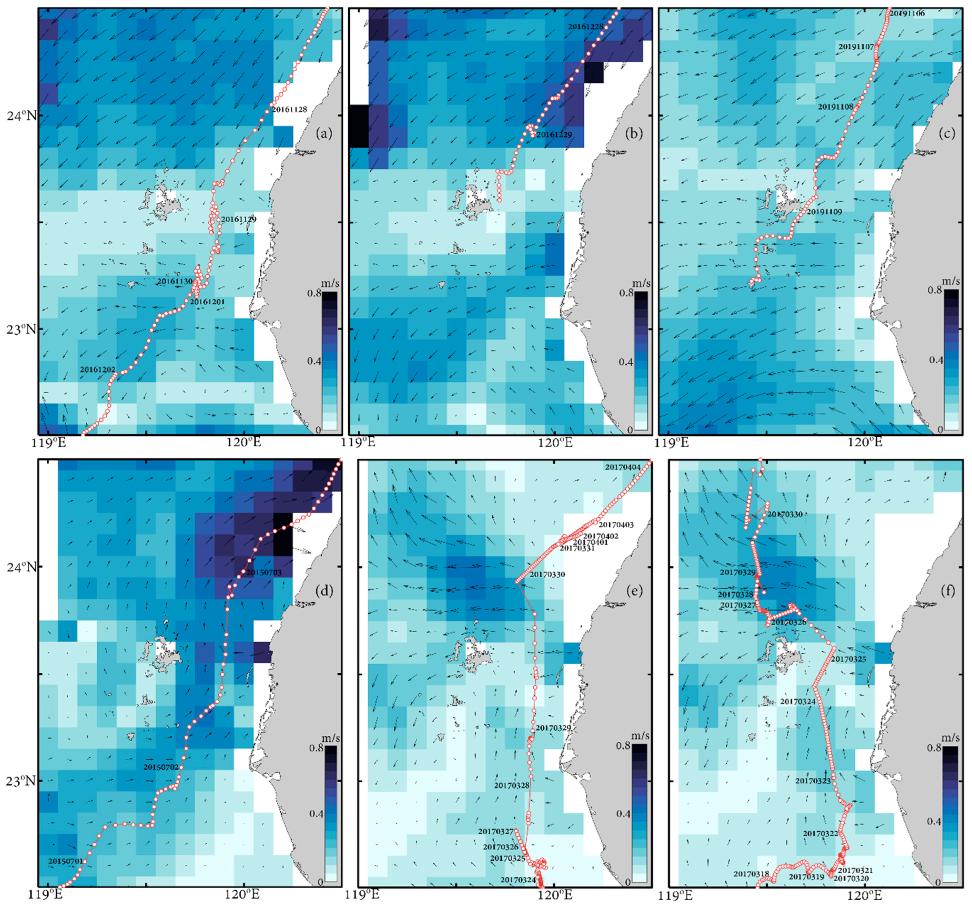
3.2. Drifter Trajectories
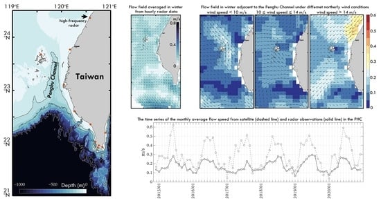
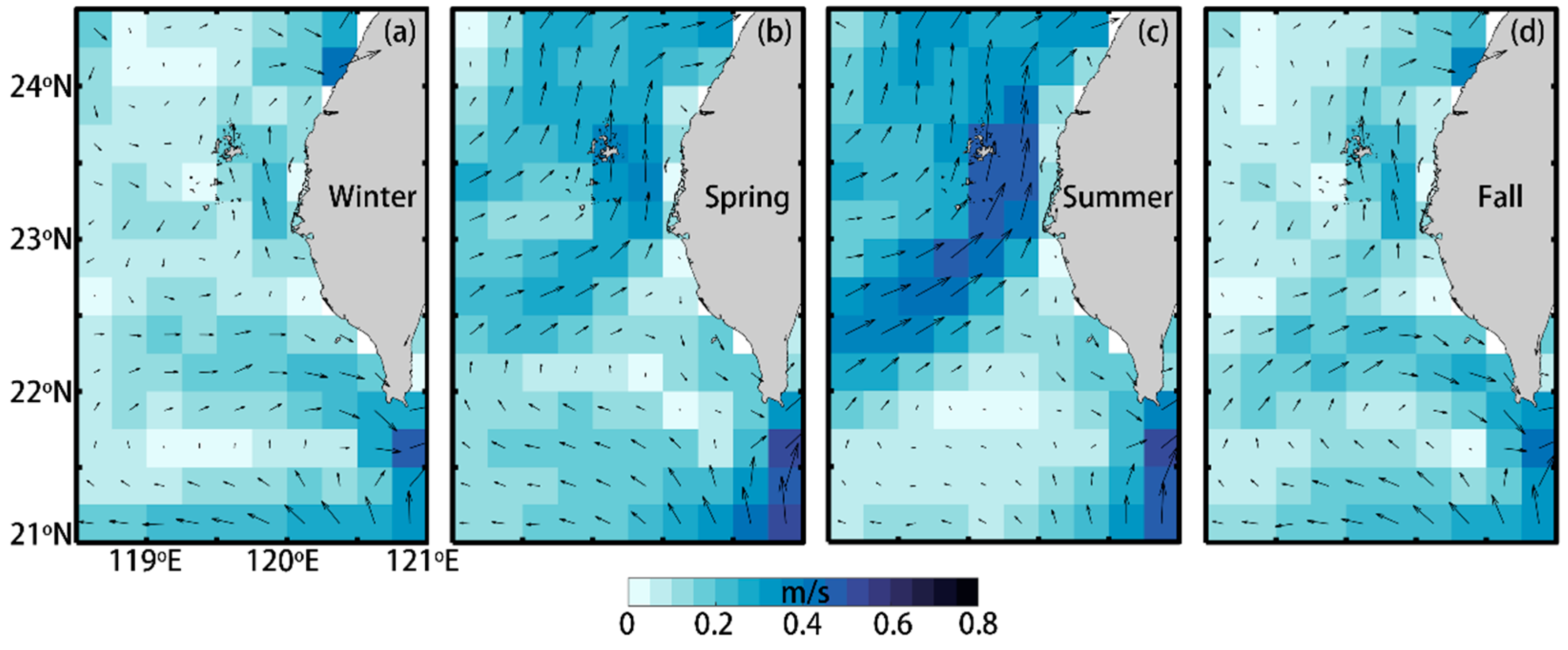
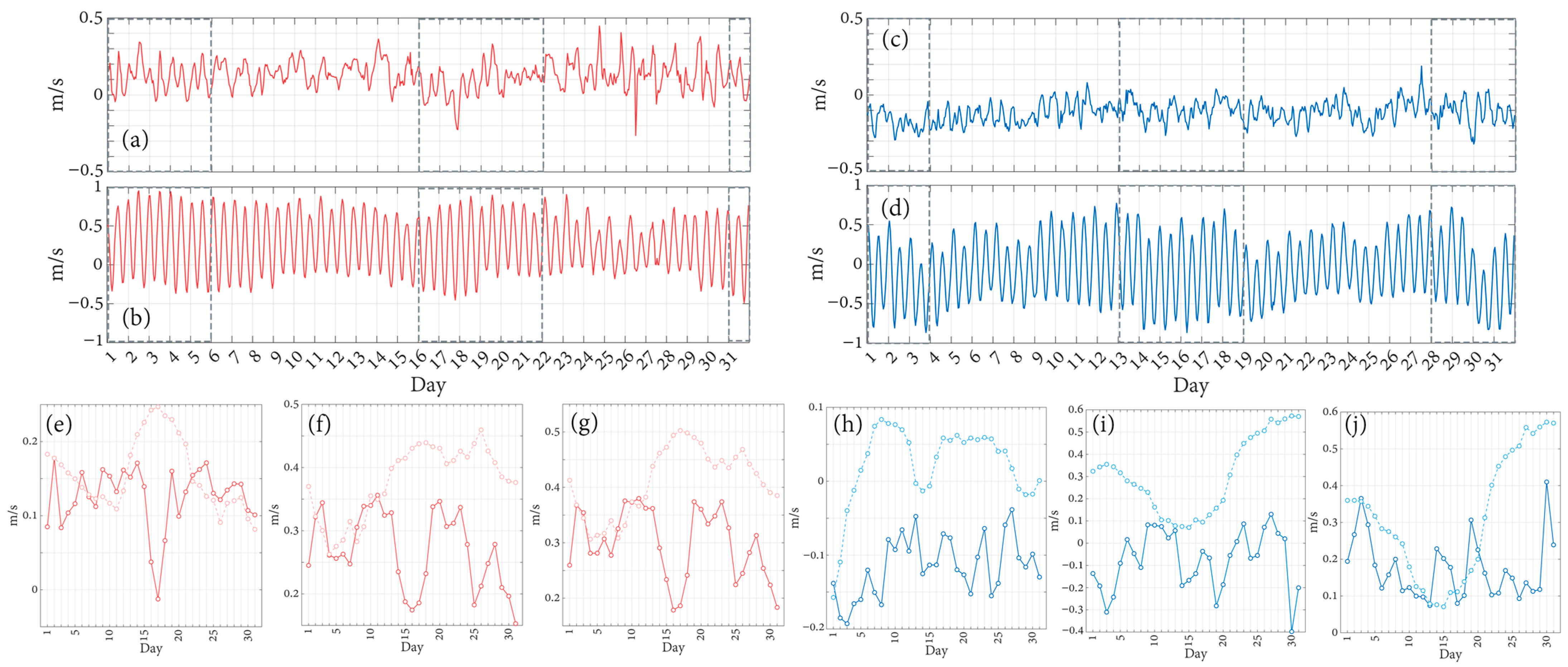
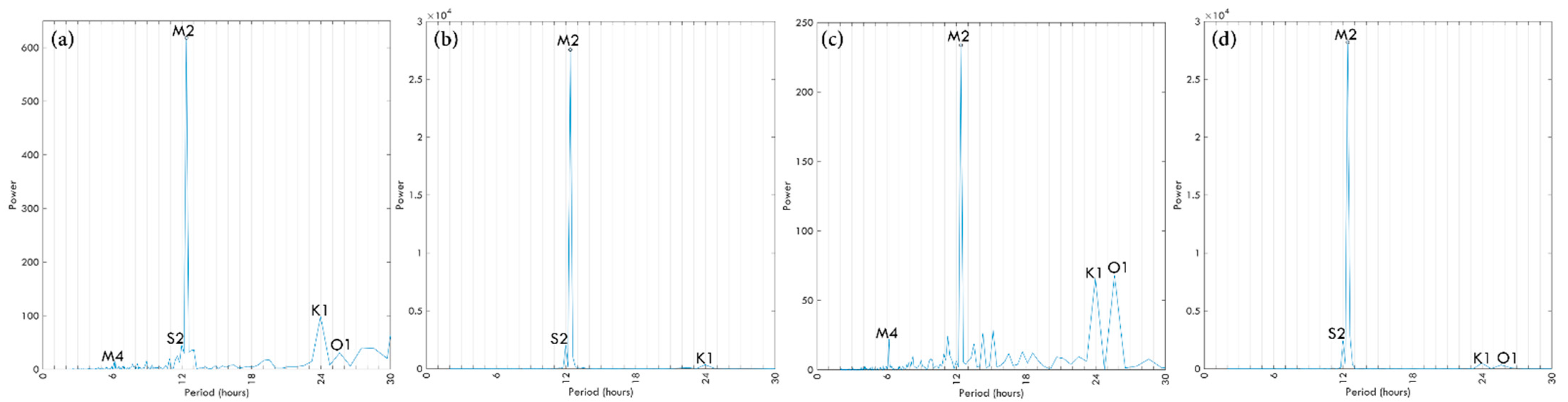
3.3. HF Radar Observations
3.4. Comparison of Ocean Surface Currents between the Satellite-Derived and HF Radar Data
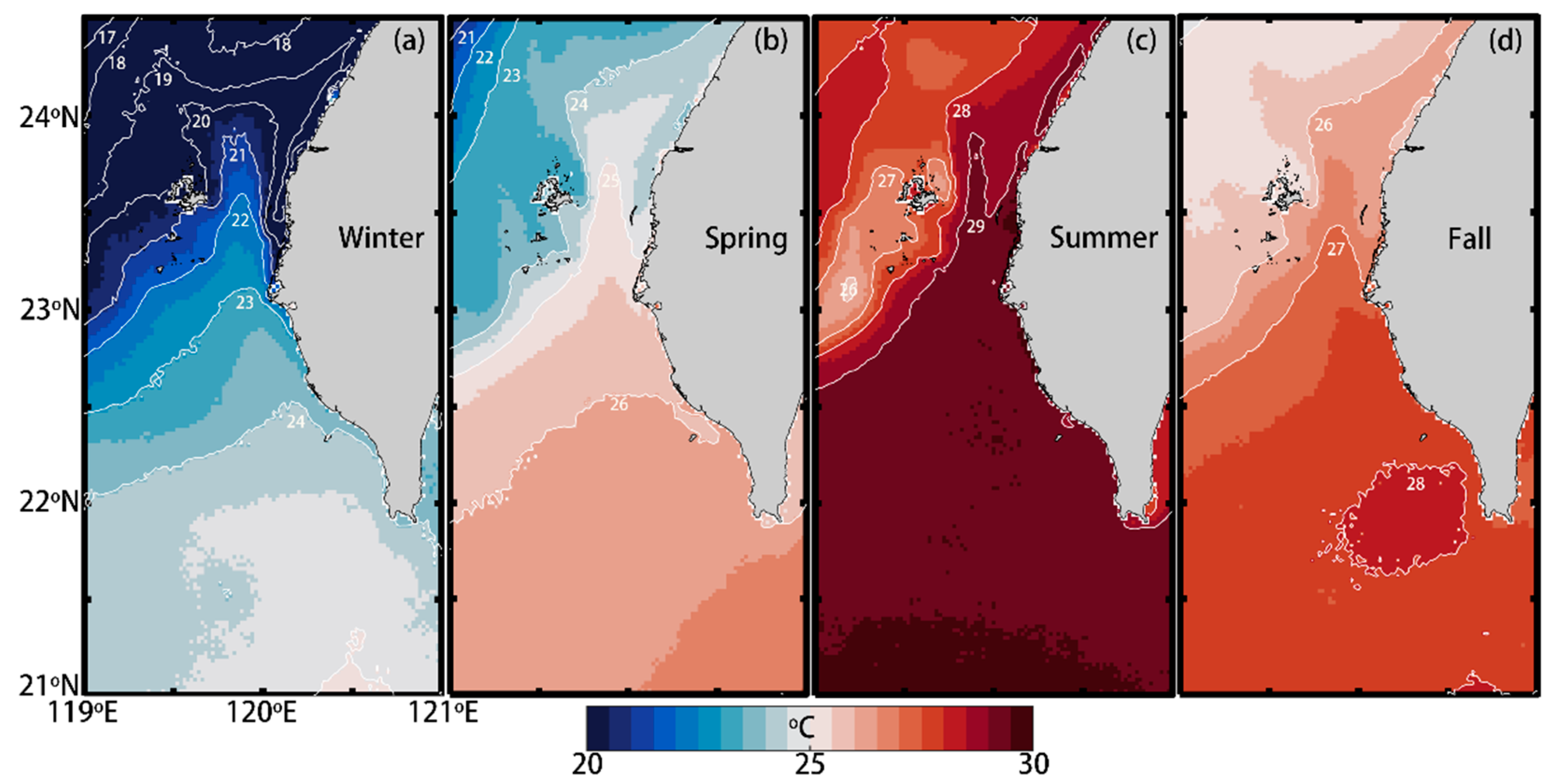
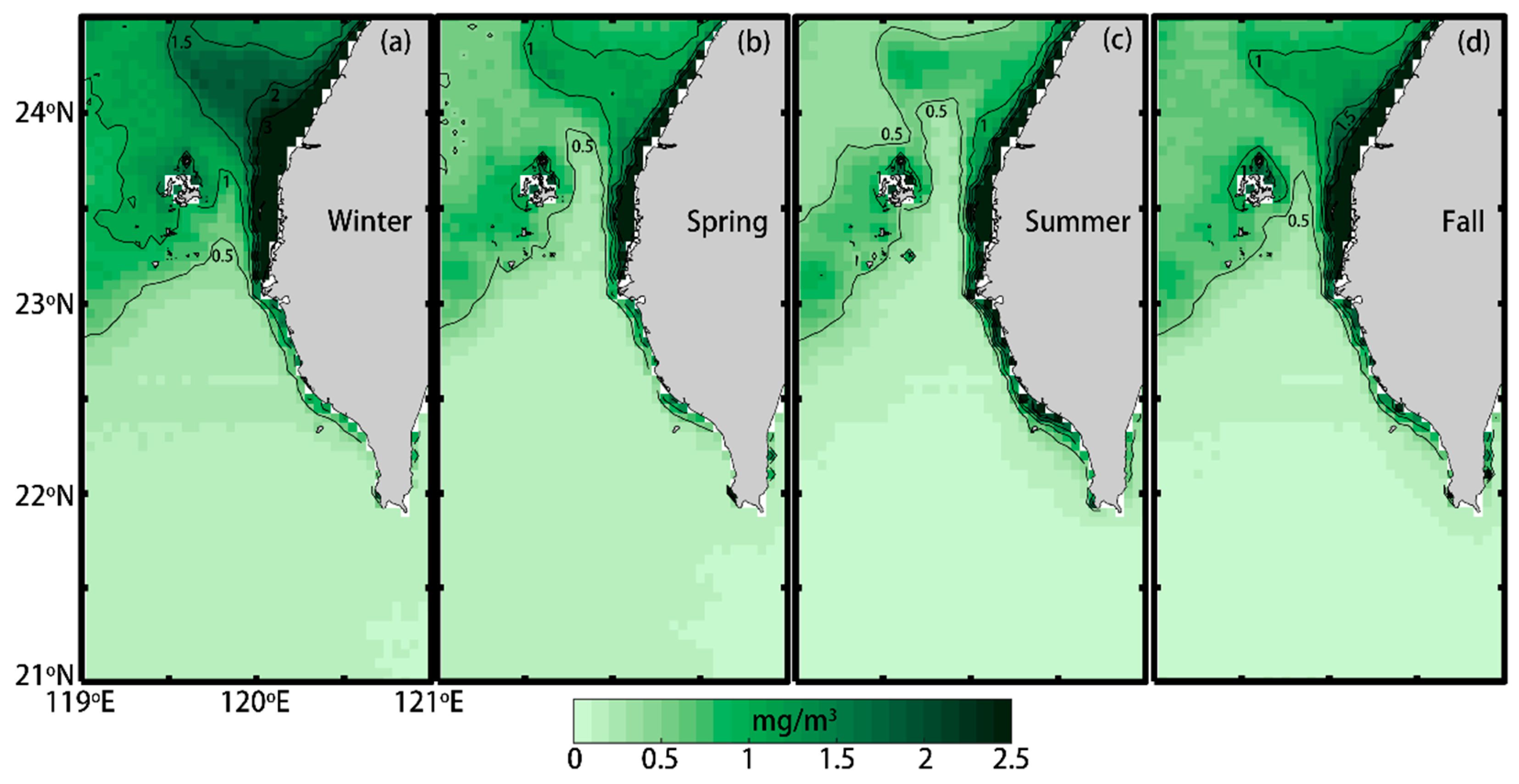
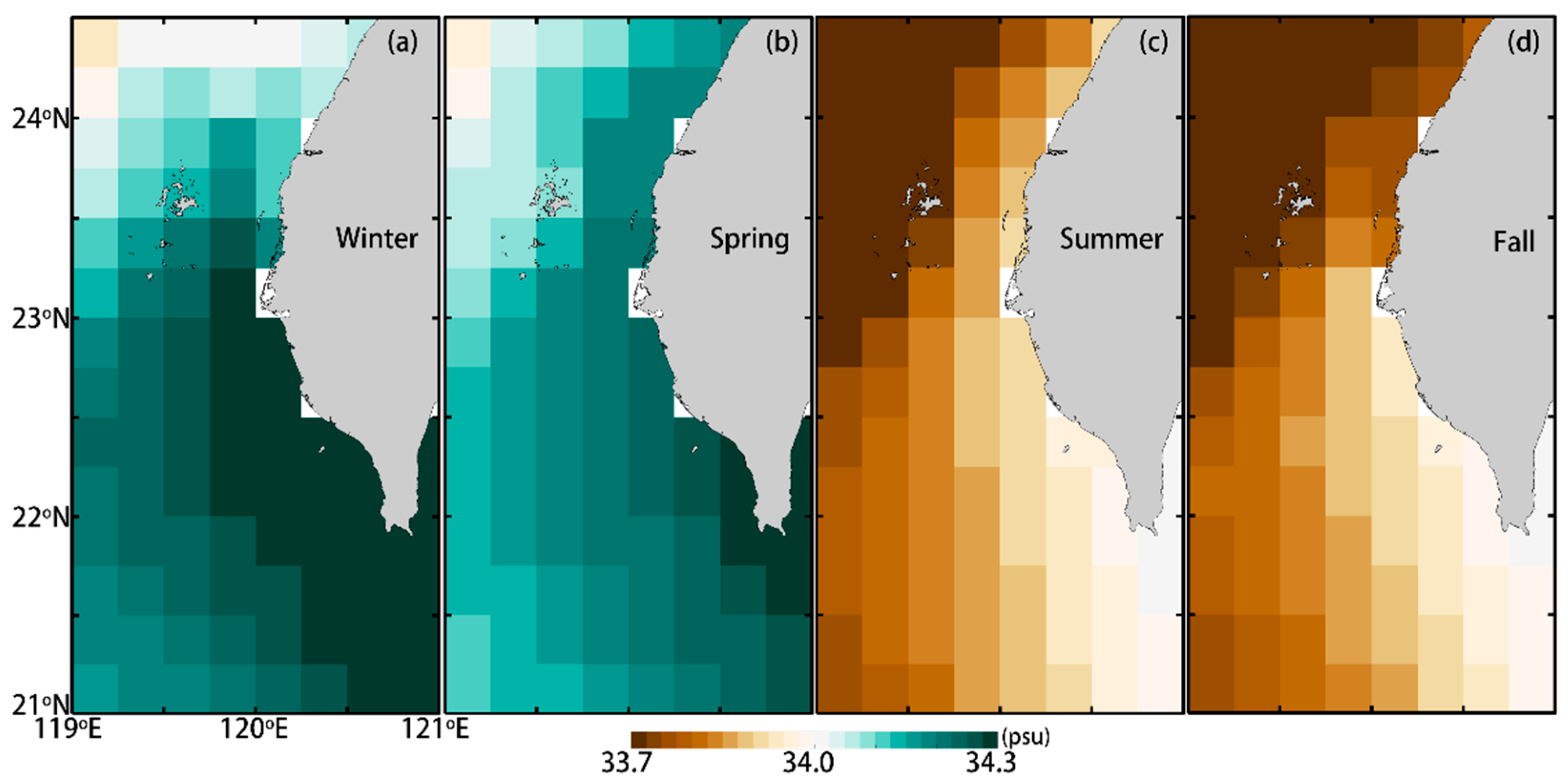
4. Hydrological Characteristics Adjacent to the PHC
5. Conclusions
Funding
Data Availability Statement
Acknowledgments
Conflicts of Interest
Appendix A


References
- Huang, Z.Y.; Yu, H.S. Morphology and geologic implications of Penghu Channel off southwest Taiwan. Terr. Atmos. Ocean. Sci. 2003, 14, 469–486. [Google Scholar] [CrossRef]
- Hsiung, K.H.; Yu, H.S.; Su, M. Sedimentation in remnant ocean basin off SW Taiwan with implication for closing northeastern South China Sea. J. Geol. Soc. 2015, 172, 641–647. [Google Scholar] [CrossRef]
- Chen, W.B.; Liu, W.C. Assessing the influence of sea level rise on tidal power output and tidal energy dissipation near a channel. Renew. Energy 2017, 101, 603–616. [Google Scholar] [CrossRef]
- Hu, Z.; Qi, Y.; He, X.; Wang, Y.H.; Wang, D.P.; Cheng, X.; Liu, X.; Wang, T. Characterizing surface circulation in the Taiwan Strait during NE monsoon from Geostationary Ocean Color Imager. Remote Sens. Environ. 2019, 221, 687–694. [Google Scholar] [CrossRef]
- Shao, H.J.; Tseng, R.S.; Lien, R.C.; Chang, Y.C.; Chen, J.M. Turbulent mixing on sloping bottom of an energetic tidal channel. Cont. Shelf Res. 2018, 166, 44–53. [Google Scholar] [CrossRef]
- Hsu, P.C.; Centurioni, L.; Shao, H.J.; Zheng, Q.; Lu, C.Y.; Hsu, T.W.; Tseng, R.S. Surface Current Variations and Oceanic Fronts in the Southern East China Sea: Drifter Experiments, Coastal Radar Applications, and Satellite Observations. J. Geophys. Res. Ocean. 2021, 126, e2021JC017373. [Google Scholar] [CrossRef]
- Fang, W.P.; Wu, D.R.; Zheng, Z.W.; Gopalakrishnan, G.; Ho, C.R.; Zheng, Q.; Huang, C.F.; Ho, H.; Weng, M.C. Impacts of the Kuroshio intrusion through the luzon strait on the local precipitation anomaly. Remote Sens. 2021, 13, 1113. [Google Scholar] [CrossRef]
- Jan, S.; Wang, J.; Chern, C.S.; Chao, S.Y. Seasonal variation of the circulation in the Taiwan Strait. J. Mar. Syst. 2002, 35, 249–268. [Google Scholar] [CrossRef]
- Lan, K.W.; Kawamura, H.; Lee, M.A.; Chang, Y.; Chan, J.W.; Liao, C.H. Summertime sea surface temperature fronts associated with upwelling around the Taiwan Bank. Cont. Shelf Res. 2009, 29, 903–910. [Google Scholar] [CrossRef]
- Bai, Y.; Huang, T.H.; He, X.; Wang, S.L.; Hsin, Y.C.; Wu, C.R.; Zhai, W.; Lui, H.K.; Chen, C.T.A. Intrusion of the Pearl River plume into the main channel of the Taiwan Strait in summer. J. Sea Res. 2015, 95, 1–15. [Google Scholar] [CrossRef]
- Kuo, Y.C.; Lee, M.A.; Chuang, C.C.; Ma, Y.P. Long-term AVHRR SST change analysis in the Taiwan Strait using the rotated EOF method. Terr. Atmos. Ocean. Sci. 2017, 28, 1–10. [Google Scholar] [CrossRef][Green Version]
- Lee, M.A.; Huang, W.P.; Shen, Y.L.; Weng, J.S.; Semedi, B.; Wang, Y.C.; Chan, J.W. Long-Term Observations of Interannual and Decadal Variation of Sea Surface Temperature in the Taiwan Strait. J. Mar. Sci. Technol. 2021, 29, 7. [Google Scholar] [CrossRef]
- Huang, T.H.; Chen, C.T.A.; Zhang, W.Z.; Zhuang, X.F. Varying intensity of Kuroshio intrusion into Southeast Taiwan Strait during ENSO events. Cont. Shelf Res. 2015, 103, 79–87. [Google Scholar] [CrossRef]
- Huang, T.H.; Lun, Z.; Wu, C.R.; Chen, C.T.A. Interannual carbon and nutrient fluxes in southeastern Taiwan Strait. Sustainability 2018, 10, 372. [Google Scholar] [CrossRef]
- Huang, T.H.; Chen, C.T.A.; Bai, Y.; He, X. Elevated primary productivity triggered by mixing in the quasi-cul-de-sac Taiwan Strait during the NE monsoon. Sci. Rep. 2020, 10, 7846. [Google Scholar] [CrossRef] [PubMed]
- Tseng, H.C.; You, W.L.; Huang, W.; Chung, C.C.; Tsai, A.Y.; Chen, T.Y.; Lan, K.W.; Gong, G.C. Seasonal variations of marine environment and primary production in the Taiwan Strait. Front. Mar. Sci. 2020, 38. [Google Scholar] [CrossRef]
- Wu, Y.L.; Lee, M.A.; Chen, L.C.; Chan, J.W.; Lan, K.W. Evaluating a suitable aquaculture site selection model for Cobia (Rachycentron canadum) during extreme events in the inner bay of the Penghu Islands, Taiwan. Remote Sens. 2020, 12, 2689. [Google Scholar] [CrossRef]
- Ko, D.S.; Chao, S.Y.; Wu, C.C.; Lin, I.I.; Sen, J. Impacts of tides and Typhoon Fanapi (2010) on seas around Taiwan. Terr. Atmos. Ocean. Sci. 2016, 27, 2. [Google Scholar] [CrossRef]
- Shen, J.; Li, L.; Zhu, D.; Liao, E.; Guo, X. Observation of abnormal coastal cold-water outbreak in the Taiwan Strait and the cold event at Penghu waters in the beginning of 2008. J. Mar. Syst. 2020, 204, 103293. [Google Scholar] [CrossRef]
- Jan, S.; Chao, S.Y. Seasonal variation of volume transport in the major inflow region of the Taiwan Strait: The Penghu Channel. Deep. Sea Res. Part II Top. Stud. Oceanogr. 2003, 50, 1117–1126. [Google Scholar] [CrossRef]
- Wu, C.R.; Hsin, Y.C. Volume transport through the Taiwan Strait: A numerical study. Terr. Atmos. Ocean. Sci. 2005, 16, 377. [Google Scholar] [CrossRef]
- Qiu, Y.; Li, L.; Chen, C.T.A.; Guo, X.; Jing, C. Currents in the Taiwan Strait as observed by surface drifters. J. Oceanogr. 2011, 67, 395–404. [Google Scholar] [CrossRef]
- Wang, L.; Pawlowicz, R.; Wu, X.; Yue, X. Wintertime Variability of Currents in the Southwestern Taiwan Strait. J. Geophys. Res. Ocean. 2021, 126, e2020JC016586. [Google Scholar] [CrossRef]
- Shen, J.; Zhang, J.; Qiu, Y.; Li, L.; Zhang, S.; Pan, A.; Huang, J.; Guo, X.; Jing, C. Winter counter-wind current in western Taiwan Strait: Characteristics and mechanisms. Cont. Shelf Res. 2019, 172, 1–11. [Google Scholar] [CrossRef]
- Tseng, Y.H.; Lu, C.Y.; Zheng, Q.; Ho, C.R. Characteristic Analysis of Sea Surface Currents around Taiwan Island from CODAR Observations. Remote Sens. 2021, 13, 3025. [Google Scholar] [CrossRef]
- Roarty, H.; Cook, T.; Hazard, L.; George, D.; Harlan, J.; Cosoli, S.; Wyatt, L.; Alvarez Fanjul, E.; Terrill, E.; Otero, M.; et al. The global high frequency radar network. Front. Mar. Sci. 2019, 6, 164. [Google Scholar] [CrossRef]
- Shen, Y.T.; Lai, J.W.; Leu, L.G.; Lu, Y.C.; Chen, J.M.; Shao, H.J.; Tseng, R.S. Applications of ocean currents data from high-frequency radars and current profilers to search and rescue missions around Taiwan. J. Oper. Oceanogr. 2019, 12, S126–S136. [Google Scholar] [CrossRef]
- Elipot, S.; Lumpkin, R.; Perez, R.C.; Lilly, J.M.; Early, J.J.; Sykulski, A.M. A global surface drifter data set at hourly resolution. J. Geophys. Res. Ocean. 2016, 121, 2937–2966. [Google Scholar] [CrossRef]
- Kurihara, Y.; Murakami, H.; Kachi, M. Sea surface temperature from the new Japanese geostationary meteorological Himawari-8 satellite. Geophys. Res. Lett. 2016, 43, 1234–1240. [Google Scholar] [CrossRef]
- Kurihara, Y.; Murakami, H.; Ogata, K.; Kachi, M. A quasi-physical sea surface temperature method for the split-window data from the Second-generation Global Imager (SGLI) onboard the Global Change Observation Mission-Climate (GCOM-C) satellite. Remote Sens. Environ. 2021, 257, 112347. [Google Scholar] [CrossRef]
- Murakami, H. Ocean color estimation by Himawari-8/AHI. In Remote Sensing of the Oceans and Inland Waters: Techniques, Applications, and Challenges; SPIE Asia-Pacific Remote Sensing: New Delhi, India, 2016; Volume 9878, pp. 177–186. [Google Scholar]
- Droghei, R.; Buongiorno Nardelli, B.; Santoleri, R. A new global sea surface salinity and density dataset from multivariate observations (1993–2016). Front. Mar. Sci. 2018, 5, 84. [Google Scholar] [CrossRef]
- Jan, S.; Sheu, D.D.; Kuo, H.M. Water mass and throughflow transport variability in the Taiwan Strait. J. Geophys. Res. Ocean. 2006, 111. [Google Scholar] [CrossRef]
- Hsu, P.C.; Lee, H.J.; Lu, C.Y. Impacts of the Kuroshio and Tidal Currents on the Hydrological Characteristics of Yilan Bay, Northeastern Taiwan. Remote Sens. 2021, 13, 4340. [Google Scholar] [CrossRef]
- Chen, C.T.A. Chemical and physical fronts in the Bohai, Yellow and East China seas. J. Mar. Syst. 2009, 78, 394–410. [Google Scholar] [CrossRef]
- Qu, B.; Song, J.; Yuan, H.; Li, X.; Li, N. Carbon chemistry in the mainstream of Kuroshio current in eastern Taiwan and its transport of carbon into the east China sea shelf. Sustainability 2018, 10, 791. [Google Scholar] [CrossRef]
- Hsu, P.C.; Ho, C.R. Typhoon-induced ocean subsurface variations from glider data in the Kuroshio region adjacent to Taiwan. J. Oceanogr. 2019, 75, 1–21. [Google Scholar] [CrossRef]


| Temperature (°C) | Salinity (psu) | |||||||
|---|---|---|---|---|---|---|---|---|
| Winter | Spring | Summer | Fall | Winter | Spring | Summer | Fall | |
| KBW | 20.4–25.4 | 19.1–27.4 | – | 22.5–28.2 | 33.9–34.8 | 33.8–34.8 | – | 33.7–34.7 |
| KIW | 5.0–12.8 | 34.2–34.4 | ||||||
| KSSW | 17.1–23.7 | 15.6–23.7 | 16.7–24.2 | 19.2–25.7 | 34.3–34.8 | 34.4–34.8 | 34.3–34.8 | 34.1–34.8 |
| MCCW | 16.4–18.6 | – | – | 22.0–24.0 | 32.7–33.9 | – | – | 31.8–33.7 |
| NTMW | 17.1–23.1 | – | – | 17.4–23.4 | 34.1–34.7 | – | – | 34.0–34.8 |
| SCSW | – | – | 21.2–30.2 | 23.7–29.5 | – | – | 33.2–34.6 | 32.6–34.3 |
| SCSSW | – | – | 26.3–29.9 | 27.8–29.2 | – | – | 32.5–33.3 | 31.4–32.6 |
Publisher’s Note: MDPI stays neutral with regard to jurisdictional claims in published maps and institutional affiliations. |
© 2022 by the author. Licensee MDPI, Basel, Switzerland. This article is an open access article distributed under the terms and conditions of the Creative Commons Attribution (CC BY) license (https://creativecommons.org/licenses/by/4.0/).
Share and Cite
Hsu, P.-C. Surface Current Variations and Hydrological Characteristics of the Penghu Channel in the Southeastern Taiwan Strait. Remote Sens. 2022, 14, 1816. https://doi.org/10.3390/rs14081816
Hsu P-C. Surface Current Variations and Hydrological Characteristics of the Penghu Channel in the Southeastern Taiwan Strait. Remote Sensing. 2022; 14(8):1816. https://doi.org/10.3390/rs14081816
Chicago/Turabian StyleHsu, Po-Chun. 2022. "Surface Current Variations and Hydrological Characteristics of the Penghu Channel in the Southeastern Taiwan Strait" Remote Sensing 14, no. 8: 1816. https://doi.org/10.3390/rs14081816
APA StyleHsu, P.-C. (2022). Surface Current Variations and Hydrological Characteristics of the Penghu Channel in the Southeastern Taiwan Strait. Remote Sensing, 14(8), 1816. https://doi.org/10.3390/rs14081816