Abstract
A high spatio-temporal resolution land surface temperature (LST) is necessary for various research fields because LST plays a crucial role in the energy exchange between the atmosphere and the ground surface. The moderate-resolution imaging spectroradiometer (MODIS) LST has been widely used, but it is not available under cloudy conditions. This study proposed a novel approach for reconstructing all-sky 1 km MODIS LST in South Korea during the summer seasons using various data sources, considering the cloud effects on LST. In South Korea, a Local Data Assimilation and Prediction System (LDAPS) with a relatively high spatial resolution of 1.5 km has been operated since 2013. The LDAPS model’s analysis data, binary MODIS cloud cover, and auxiliary data were used as input variables, while MODIS LST and cloudy-sky in situ LST were used together as target variables based on the light gradient boosting machine (LightGBM) approach. As a result of spatial five-fold cross-validation using MODIS LST, the proposed model had a coefficient of determination (R2) of 0.89–0.91 with a root mean square error (RMSE) of 1.11–1.39 °C during the daytime, and an R2 of 0.96–0.97 with an RMSE of 0.59–0.60 °C at nighttime. In addition, the reconstructed LST under the cloud was evaluated using leave-one-station-out cross-validation (LOSOCV) using 22 weather stations. From the LOSOCV results under cloudy conditions, the proposed LightGBM model had an R2 of 0.55–0.63 with an RMSE of 2.41–3.00 °C during the daytime, and an R2 of 0.70–0.74 with an RMSE of 1.31–1.36 °C at nighttime. These results indicated that the reconstructed LST has higher accuracy than the LDAPS model. This study also demonstrated that cloud cover information improved the cloudy-sky LST estimation accuracy by adequately reflecting the heterogeneity of the relationship between LST and input variables under clear and cloudy skies. The reconstructed all-sky LST can be used in a variety of research applications including weather monitoring and forecasting.
1. Introduction
Land surface temperature (LST) is the radiative temperature of the Earth’s surface. LST plays a key role in the energy balance between the atmosphere and the ground surface [1,2]. A high spatiotemporal resolution LST is widely required for various research fields such as heat flux monitoring, the biogeochemical cycle, and land surface process modeling [3,4,5,6,7]. Therefore, it is essential to produce spatiotemporally seamless LST in an accurate manner.
LST can be monitored with high temporal resolution at weather stations. However, LST measured at weather stations is point-scale, inherently aspatial. The number of weather stations is insufficient due to the considerable labor and cost associated with their management and maintenance [8]. So, there is a limitation on spatially monitoring LST based on weather stations in vast areas, particularly when topographical complexity is high. Owing to the exponential growth of satellite remote sensing fields over the past decades, LST can be retrieved with high accuracy of 1–2 K using thermal infrared (TIR) sensors over large areas [2].
Therefore, satellite-based LST has been utilized more than weather station-measured LST in many studies [9,10,11,12,13]. Among various satellite-based LSTs, the moderate-resolution imaging spectroradiometer (MODIS) satellite-based LST has been widely utilized because of its 1 km spatial resolution and four-times-a-day temporal resolution. Unfortunately, MODIS or other TIR-based LST cannot be used under cloudy conditions, often problematic in humid areas [5,14,15,16,17]. Thus, TIR-based LSTs typically contain a large number of missing pixels.
Under cloudy conditions, there are four typical methods for filling missing LST pixels. The first is the gap-filling method that adopts the spatial and temporal information of neighboring clear-sky LST pixels to interpolate missing cloudy-sky LST pixels [18,19,20,21]. It uses spatial and temporal correlations between the missing and adjacent pixels. However, cloud effects on LST exist, with a cooling effect during the daytime due to a decrease in downwelling shortwave radiation and a warming effect at nighttime due to an increase in downwelling longwave radiation [22,23]. As the gap-filling method replaces the missing LST with the spatially and temporally neighboring clear-sky LST pattern, it is difficult to reflect the cloud effects on LST. The second is the surface energy balance (SEB) technique, which estimates the LST under the cloud by calculating the difference between clear-sky and cloudy-sky pixels using the SEB equation [24,25,26,27,28]. However, complex parameterization of air temperature and wind speed is required for the SEB technique. In addition, since its performance depends on input shortwave radiation (SR), it is difficult to apply the SEB technique at night when SR does not contribute to the spatial variation of LST.
The third approach is to use passive microwave (PMW) satellite data. Due to its ability to penetrate water vapor and the cloud, PMW has the advantage of acquiring all-sky surface information. For example, the advanced microwave scanning radiometer 2 (AMSR2) brightness temperature has been used to retrieve LST. Numerous all-sky 1 km MODIS LST reconstruction methods have been developed through the fusion of MODIS and AMSR2 data, including physical, semi-empirical, empirical, and machine learning approaches [29,30,31,32,33]. However, the temperature retrieved from PMW is not the surface temperature but rather the subsurface temperature [34]. In addition, PMW-derived LST has low spatial and temporal resolutions (10–25 km and approximately 1 to 2 days) compared to MODIS LST.
The fourth approach is to use numerical models, which can produce all-sky LST with high temporal resolution. Although numerical model-derived LST is spatially smoothed to reduce grid-scale noise, using such LST as input data in statistical models has been an alternative approach for LST gap-filling [35,36]. Many previous studies have frequently used Global Land Data Assimilation System (GLDAS) models due to their ability to cover a large area without introducing spatial gaps [37,38,39]. However, GLDAS has a coarser spatial resolution of 0.25° than MODIS. In areas with complex topography, it is necessary to use high-resolution numerical models such as weather research and forecasting (WRF), which can monitor mesoscale weather phenomena in local areas.
Many studies have reconstructed all-sky 1 km MODIS LST based on machine learning approaches because they can consider non-linear relationships among input and target variables [14,36,40]. Most previous studies modeled a relationship between predictand variables and clear-sky LST, and then applied it to cloudy conditions. However, the relationship varies by sky conditions (i.e., cloudy or clear). To deal with such a problem, both Yoo et al. (2020) and Li et al. (2021) conducted all-sky LST reconstruction by training machine learning models using in situ cloudy-sky LST observations [15,37]. These studies found that the use of in situ cloudy-sky LST observations can be beneficial to the consideration of the cloud effects on LST in all-sky LST reconstruction models. However, due to the sparse distribution of in situ measurements, relying exclusively on in situ observations may limit spatial representation. Thus, it is necessary to develop an effective all-sky 1 km MODIS LST reconstruction approach that combines MODIS and in situ cloudy-sky LSTs and high-resolution numerical models.
This study aims to construct an all-sky 1 km MODIS LST over South Korea using the light gradient boosting machine (LightGBM) approach, considering the cloud effects on LST. LightGBM uses a gradient boosting framework with high computational speed and efficient memory usage without compromising performance. MODIS data, in situ observations, and the high-resolution Local Data Assimilation and Prediction System (LDAPS) output were used for MODIS LST reconstruction. The proposed approach is expected to produce reliable all-sky LST by considering the relationships between LST and predictand variables both under clear and cloudy skies. The key objectives of this study were to (1) develop an all-sky 1 km MODIS LST reconstruction model, (2) evaluate the developed model based on systematic validations using two different LST sources (i.e., MODIS LST and in situ observations), and (3) examine whether the model incorporating the cloud effect improves the estimation accuracy of cloudy-sky LST.
2. Study Area and Data
2.1. Study Area
The study area is South Korea (~99,840 km2; 124°–130°E, 33°–39°N), which is located in Northeast Asia (Figure 1). South Korea has a hot and humid summer owing to the North Pacific air mass and cold winters due to dry continental high pressure. The annual mean temperature in South Korea is approximately 10–15 °C, with a mean temperature of 23–26 °C in August, the hottest month. Additionally, due to the East Asian monsoon, it experiences extremely humid summers with concentrated precipitation (i.e., the annual rainfall was 1306.3 mm on average across 1991–2020 with a mean summer rainfall of 710.9 mm). This results in a high cloud cover rate in South Korea during the summer. Therefore, this research focused on summer seasons (i.e., June to August across 2013–2020).
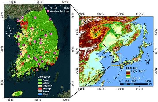
Figure 1.
Study area and spatial distribution of the weather stations used in this study. Station numbers are labeled in order of decreasing latitude. Elevation is derived from Shuttle Radar Topography Mission (SRTM) digital elevation model (DEM) with 90 m spatial resolution. Land cover is extracted from the MODIS land cover with 500 m spatial resolution for 2019.
2.2. MODIS Data
This study used daily MODIS LST products (MOD11A1 for Terra and MYD11A1 for Aqua) with a spatial resolution of 1 km. The MODIS LST is retrieved from two different TIR bands (i.e., band 31 with 10.78–11.28 μm and band 32 with 11.77–12.27 μm) via a generalized split-window algorithm [41]. Terra MODIS provides LST observed at 10:30 a.m. and 10:30 p.m., and Aqua MODIS provides LST observed at 1:30 p.m. and 1:30 a.m. local time. The MODIS LST data from 2013 to 2020 were obtained through Earthdata Search (https://search.earthdata.nasa.gov/search; assessed on 1 August 2020). In addition, annual MODIS land cover (MCD12Q1) was employed for data processing and analysis.
2.3. In Situ LST Data
Hourly in situ LST observations (i.e., 1 a.m./p.m., 2 a.m./p.m., 10 a.m./p.m., and 11 a.m./p.m.) were acquired from automated surface observing systems (ASOS) managed by the Korea Meteorological Administration (KMA). ASOS provides LST data measured directly at 0 cm via a platinum resistance temperature sensor. There are 102 ASOSs in South Korea, but the stations that changed their location between 2013 and 2020 were excluded. In addition, we excluded the stations with a calibration error (root mean square error; RMSE) >3 °C from the bias correction described in Section 3.1 to minimize the spatial discrepancy between in situ measurements and satellite data. Finally, data collected from a total of 22 ASOS stations were used in this study.
2.4. LDAPS Model Data
The KMA is currently operating the LDAPS model based on UK Met Office’s Unified Model (UM model), which uses non-hydrostatic dynamics, semi-Lagrangian advection, and semi-implicit time-stepping [42]. LDAPS uses the Global Data Assimilation and Prediction System (GDAPS) with a coarse spatial resolution of 10–25 km as initial and boundary conditions. LDAPS produces analysis data eight times a day with 3 h intervals (i.e., 0, 3, 6, 12, 15, 18, and 21 UTC). It has a spatial resolution of 1.5 km and 70 vertical levels in the Korean Peninsula and the surrounding seas. This study used several surface grid data from LDAPS: LST and four parameters—air temperature (Tair), relative humidity (RH), wind speed (WS), and precipitation (Ppt)—closely related to the spatio-temporal changes of LST [43].
2.5. Auxiliary Data
The elevation, slope, impervious area ratio, mean WS, day of the year (DOY), longitude, and latitude were used as auxiliary variables to consider the spatial and temporal variation of LST. The elevation, slope, and impervious area ratio provide information on topography and landcover that affect the spatial variability of LST [43,44]. Elevation was constructed from the Shuttle Radar Topography Mission (SRTM) Digital Elevation Model (DEM) with a spatial resolution of 90 m (https://earthexplorer.usgs.gov; assessed on 1 August 2021). The slope was retrieved using DEM data with the “Slope” tool of Spatial Analyst Toolbox in ArcGIS. The Global Human Settlement (GHS) built-up dataset with a 250 m spatial resolution was employed as built-up area information (https://ghsl.jrc.ec.europa.eu/ghs_bu2019.php; assessed on 1 August 2021). The mean WS was extracted from the Global Wind Atlas, which offers local wind climates with a 250 m spatial resolution. Longitude and latitude were also extracted from the grid of MODIS LST to account for clear-sky LST pixels in the vicinity of missing LST under the cloud. Lastly, DOY was used after conversion to a range between −1 and 1 through cosine transformation to represent the temporal variability of LST.
3. Methods
3.1. Data Processing
This study used the MODIS LST time series filtered to include only high-quality data via the quality flag. However, since MODIS LST is of lower quality in built-up areas than in other land covers [45], there are insufficient samples for a machine learning model to learn LST characteristics in built-up areas. To develop an LST reconstruction model that can reflect all land surface characteristics in the study area, this study used MODIS LST in the built-up areas without the quality-screening process. In addition, the MODIS quality flag contains information about the existence of clouds in each pixel. We extracted the cloud cover from the MODIS quality flag and used it to consider the varied relationship between LST and input variables on clear and cloudy skies.
The LDAPS data with 3 h intervals were linearly interpolated to the MODIS observation time and bilinearly resampled to 1 km spatial resolution. The hourly observed in situ LST was also linearly interpolated to match the MODIS view time. The point-scale in situ LST measurements showed a trend of increasing more rapidly than the 1 km MODIS LST at high temperatures in summer. To reduce the spatial scale discrepancy between MODIS LST and in situ observations, a polynomial regression-based bias correction was applied [15]. Considering the distribution range of daytime LST lowered by cloud in summer, MODIS and in situ LSTs from May to October were used for the bias correction.
Figure 2 summarizes the entire procedure of this study. The LDAPS model’s analysis data (i.e., LST, Tair, RH, WS, and Ppt), binary MODIS cloud cover, and seven auxiliary variables (i.e., elevation, slope, impervious area ratio, mean WS, DOY, longitude, and latitude) were used as input data, while the MODIS LST and bias-corrected in situ cloudy-sky LST were used as reference data. The MODIS LST was sampled over the entirety of South Korea, while the cloudy-sky LST was collected from 22 ASOS stations. Using LightGBM, an all-sky MODIS LST reconstruction model was developed for each MODIS view time.
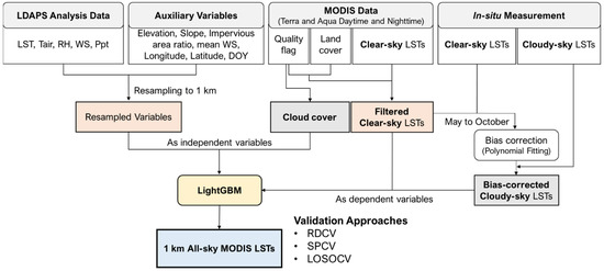
Figure 2.
Flowchart of the LightGBM-based all-sky 1 km MODIS LST reconstruction model proposed in this study.
3.2. Light Gradient Boosting Machine
Ensemble machine learning approaches (e.g., random forest (RF) and extreme gradient boosting (XGBoost)) have been widely used for producing an all-sky LST in many previous studies [14,36,40]. Both RF and XGBoost grow multiple decision trees and then average their outputs to obtain a final prediction for regression, generally yielding better performance than single decision trees. However, they are slow and ineffective when training with a large number of samples [46]. One solution to this problem is to reduce the number of samples, but there is no clear method for optimizing data sampling.
LightGBM was proposed to accelerate the training process without a reduction in accuracy [47,48]. LightGBM belongs to the Gradient Boosting Decision Tree (GBDT) algorithm, which approximates a gradient decent step in the direction of minimizing the loss function (residual errors). Existing GBDT methods (e.g., XGBoost) use a level-wise tree growth strategy that keeps the trees balanced, which often takes a great deal of time to optimize. On the other hand, LightGBM uses the leaf-wise tree growth strategy, which splits the leaf with the most loss and does not bother the remaining leaves on the same level, saving processing time. Additionally, LightGBM employs Gradient-Based One Side Sampling (GOSS), a sampling method based on gradients. The key concept of GOSS is that the instances with large gradients contribute much more to growing a decision tree than those with small gradients. Consequently, GOSS keeps the instances with large gradients, but it performs random sampling on those with small gradients. Through the leaf-wise tree growth strategy and GOSS, LightGBM has a fast training speed with low memory consumption and often performs better than other boosting algorithms [47,49]. Therefore, this study adopted LightGBM to produce all-sky LST for a relatively long-term period (i.e., 2013–2020), with more than 10 million samples per MODIS view time [50,51].
We implemented LightGBM using the ‘lightgbm’ package in Python. The hyperparameters of LightGBM include max_depth, min_data_in_leaf, num_leaves, and n_estimators. The max_depth parameter presents the maximum depth of a tree. The min_data_in_leaf and the num_leaves parameters determine the minimum number of samples in a leaf and the number of leaves, respectively. These three parameters control the overfitting of the LightGBM model. Lastly, the n_estimators parameter indicates the number of trees. Table 1 shows the combination of hyperparameters tested for model optimization in this study. The LightGBM optimization process in this study is described in Section 3.3.

Table 1.
Various combinations of hyperparameters tested to optimize the proposed LightGBM model.
3.3. Performance Evaluation of the Proposed Approach
Three different cross-validation approaches were conducted to evaluate the robustness and generalization of the proposed model. First, random five-fold cross-validation (RDCV) was performed using MODIS LST to evaluate the reconstructed clear-sky LST. To evaluate the spatial distribution of the simulated LST, spatial five-fold cross-validation (SPCV) was also conducted. Finally, leave-one-station-out cross-validation (LOSOCV) using 22 ASOSs was performed to evaluate the estimated cloudy-sky LST. In the cross-validation process, the training and validation sets were randomly divided by 8:2 from the total dataset, except for the independent test data. For example, RDCV randomly divided the total dataset into five subsets, where one subset was used for test data and the remaining four subsets were divided again by 8:2 for training and validation. The optimal hyperparameters were selected based on the lowest validation RMSE (Equation (1)) through the grid search method. This process was repeated five times, and then RDCV performance was obtained by averaging the test result for each fold. This hyperparameter tuning and evaluation approach based on cross-validation has been widely adopted in recent studies that used machine learning [52,53,54].
The proposed model was compared with temporally spline-interpolated LDAPS LST considering its diurnal cycle pattern [55]. The coefficient of determination (R2; Equation (2)), bias (difference; Equation (3)), RMSE, and relative RMSE (rRMSE; Equation (4)) were used for accuracy assessment.
where and are measured and predicted values, respectively.
In addition, this study analyzed the effects of the learning strategy using in situ cloudy-sky LST as a target variable and the cloud cover as the input variable for cloudy-sky LST estimation. Two scenarios—LightGBM without both in situ cloudy-sky LST and cloud cover data (scenario 1) and LightGBM without cloud cover data (scenario 2)—were further compared to the proposed LightGBM model with all input variables.
4. Results
Figure 3 shows the two cross-validation results (i.e., RDCV and SPCV) of LDAPS and the proposed LightGBM model using Terra and Aqua daytime and nighttime clear-sky LST during the summer seasons. LDAPS showed an R2 of 0.30–0.35 and RMSE of 3.61–4.54 °C during the daytime, and an R2 of 0.70–0.80 and RMSE of 2.30–2.38 °C at nighttime. On the other hand, the RDCV result of LightGBM had an R2 of 0.93 and RMSE of 0.95–1.16 °C during the daytime, and an R2 of 0.96–0.97 and RMSE of 0.56–0.58 °C at nighttime, yielding higher estimation accuracy than LDAPS for all different MODIS view times. The SPCV result showed a slightly lower accuracy than the RDCV, but still showed low RMSE values ≤1.4 °C and 0.6 °C during the daytime and nighttime, respectively.
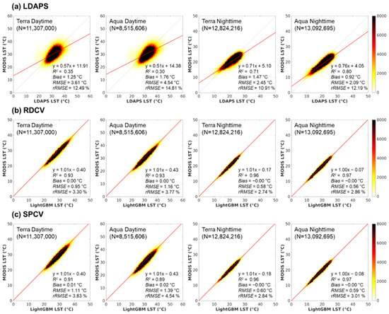
Figure 3.
Performances of (a) LDAPS and the proposed LightGBM model’s (b) RDCV and (c) SPCV for four clear-sky MODIS LSTs (i.e., Terra and Aqua for daytime and nighttime).
We analyzed the spatial difference between the LSTs from the LDAPS and LightGBM models and MODIS LST (Figure 4). LDAPS showed a generally higher LST distribution than MODIS over most of the study area. In particular, LDAPS provided much higher LST than MODIS in urban areas during both day and night, but significantly lower LST than MODIS in coastal areas during the daytime. This might be because GDAPS with a 10–25 km coarse spatial resolution is used as the initial conditions of LDAPS, resulting in high uncertainty and variation in coastal areas. On the other hand, the proposed LightGBM had similar spatial distribution as MODIS LST, yielding little difference between the two.
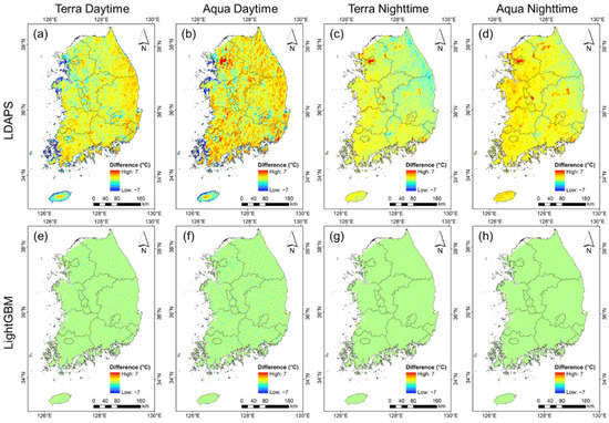
Figure 4.
LST difference between the (a–d) LDAPS and (e–h) the proposed LightGBM model for four clear-sky LSTs (i.e., Terra and Aqua for daytime and nighttime). The difference maps of the LightGBM model were produced from the SPCV results.
The performances of LDAPS and LightGBM by land cover are depicted in Figure 5. The LightGBM outperformed LDAPS in the four different land covers for all MODIS view times, producing higher R2 and lower RMSE. Except for built-up areas, the proposed LightGBM model had an R2 ≥ 0.80 and RMSE ≤ 1.6 °C during the daytime, and an R2 ≥ 0.95 and RMSE ≤ 0.7 °C at nighttime. Among four different land covers, the LightGBM model generally had the highest accuracy in forest areas but was less accurate in the built-up class than other land covers.
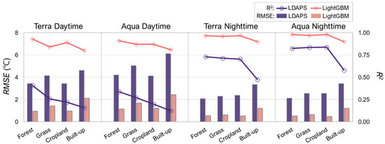
Figure 5.
Performance of the LDAPS and the proposed LightGBM model by land cover for four clear-sky LSTs (i.e., Terra and Aqua for daytime and nighttime). The performance of the LightGBM model by land cover was calculated from the SPCV results.
The clear and cloudy-sky LSTs provided by the LDAPS and the proposed LightGBM model were evaluated through LOSOCV using the bias-corrected in situ LST from the 22 ASOS stations (Table 2). The clear-sky MODIS LST was also compared. Among them, LDAPS showed the highest RMSE at both daytime and nighttime, while relatively high R2 values of 0.77–0.82 at nighttime. On the other hand, LightGBM showed the lowest RMSE of 2.40–2.70 °C and 1.33–1.45 °C during the daytime and nighttime, respectively. Although LightGBM showed a relatively low correlation with in situ LST during the daytime, it produced an R2 similar to MODIS.
Table 2.
LOSOCV results for LSTs from MODIS, LDAPS, and the proposed LightGBM models under clear and cloudy-sky conditions against the bias-corrected in situ LST measurements at 22 ASOSs in June–August from 2013 to 2020.
Under cloudy conditions, LDAPS had an R2 of 0.54–0.59 and RMSE of 2.84–3.34 °C during the daytime, while it yielded an R2 of 0.72–0.75 with RMSE of 1.96–2.21 °C at nighttime. On the contrary, LightGBM had an R2 similar to LDAPS but lower RMSE of 2.41–3.00 °C during the daytime and 1.31–1.36 °C at nighttime. We further compared the RMSE of LDAPS and LightGBM for four cloudy-sky LSTs at each station (Figure 6). LightGBM resulted in lower RMSE values than LDAPS at most stations under cloudy conditions for all four MODIS view times. Additionally, we analyzed the temporal variation of LST estimated by the LDAPS and LightGBM models at station 8 in August 2013, when it was very hot with a high cloud cover rate (Figure S1). For all four MODIS view times, LDAPS tended to overestimate LST compared to the in situ measurements. On the other hand, LightGBM showed good agreement with the in situ LST without such a bias.
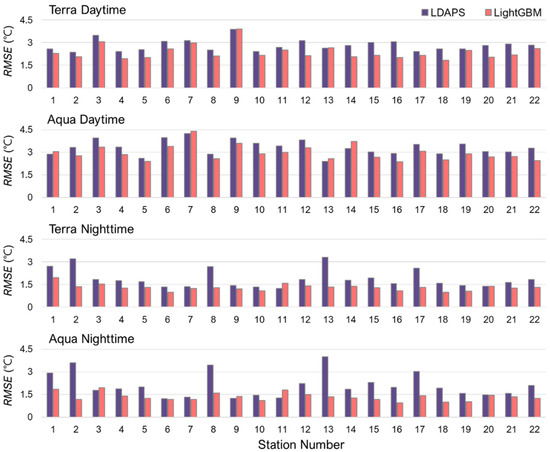
Figure 6.
RMSEs for cloudy-sky LSTs from the LDAPS and proposed LightGBM models against the bias-corrected in situ LST measurements for each ASOS. Please refer to Figure 1 for station numbers.
Figure 7 and Figure 8 depict the spatial maps of the average all-sky 1 km LST of the LDAPS and LightGBM models for daytime and nighttime, respectively, in June–August from 2013 to 2020. The daytime and nighttime LSTs of both models showed a negative spatial relationship with elevation (see Figure 1). While LDAPS showed a relatively smoothed spatial pattern of LST, LightGBM produced spatially detailed LST distribution. Figure 9 displays the original MODIS LSTs and the corresponding all-sky LSTs of LDAPS and LightGBM at both daytime and nighttime on 6 August 2016. As shown in Figure 4, the daily LST difference between MODIS and LDAPS was evident. Although the overall LST spatial patterns of LDAPS were similar to MODIS, they were spatially smoothed. On the contrary, the proposed model successfully filled the missing LST pixels without the smoothing effect.
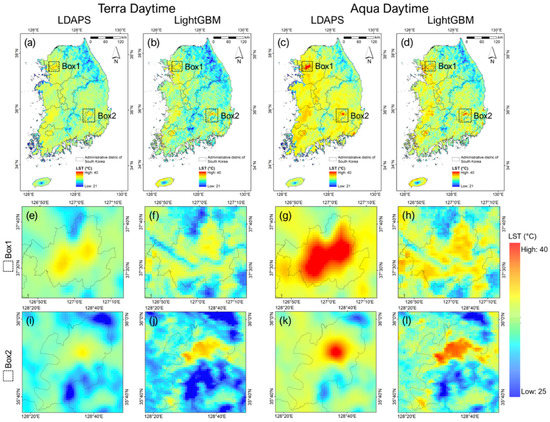
Figure 7.
Spatial distribution of the average all-sky 1 km LSTs for Terra and Aqua daytime produced by (a,c) LDAPS and (b,d) LightGBM in June–August from 2013 to 2020. The enlarged LST distributions of (e,g,i,k) LDAPS and LightGBM (f,h,j,l) are shown for two subset areas (i.e., boxes 1 and 2), which are representative metropolitan areas in South Korea that often suffer from summer heatwaves.
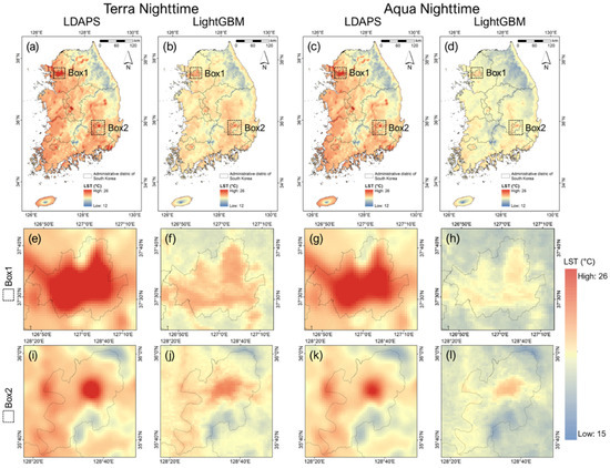
Figure 8.
Spatial distribution of the average all-sky 1 km LSTs for Terra and Aqua nighttime produced by (a,c) LDAPS and (b,d) LightGBM in June–August from 2013 to 2020. The enlarged LST distributions of (e,g,i,k) LDAPS and (f,h,j,l) LightGBM are shown for two subset areas (i.e., boxes 1 and 2), which are representative metropolitan areas in South Korea that often suffer from summer heatwaves.
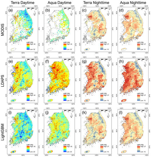
Figure 9.
Spatial distribution of 1 km LSTs from (a–d) MODIS, (e–h) LDAPS, and (i–l) LightGBM for four MODIS view times (i.e., Terra and Aqua for daytime and nighttime) on 6 August 2018.
5. Discussion
5.1. Model Evaluation Using MODIS LST and In Situ LSTs
The performances of the LDAPS and LightGBM models during the daytime were lower than at night (Figure 3). In particular, both models showed the highest rRMSE for Aqua daytime and the lowest rRMSE for Aqua nighttime. This result is because the daytime LST becomes more unstable than the nighttime LST due to downward solar radiation, which causes a more heterogeneous spatial thermal distribution on the land surface in the daytime [5,37,56]. Unlike the proposed model, LDAPS showed a significant performance difference between day and night of up to 2 °C RMSE. LDAPS has a spatially smoothed thermal distribution due to the surface properties roughly considered in the model [57,58,59], which may result in a high error during the daytime with a relatively high spatial variation in the thermal distribution.
In addition, the LDAPS LST showed a high spatial difference compared to the MODIS LST (Figure 4), which could be because LDAPS considers land cover types but does not adequately account for environmental variables such as vegetation abundance and soil moisture [60]. On the other hand, the LightGBM-derived LST showed a spatial distribution very similar to that of MODIS. These results imply that the proposed model produced MODIS-like LST well under clear-sky conditions. Among several types of vegetation, the LightGBM model generally had the highest accuracy in forest areas, with relatively lower performance in grass and cropland areas (Figure 5). This result is consistent with previous studies [15,37]. The built-up class showed a relatively low accuracy compared to other land covers, which may be due to the high uncertainty of MODIS LST over urban areas [19,45].
Clear-sky LSTs from MODIS, LDAPS, and LightGBM showed a relatively low correlation with the bias-corrected in situ observations during the daytime (Table 2). To analyze the low correlation between MODIS and in situ LSTs under clear-sky conditions during the daytime, we analyzed the correlation between the clear-sky LST observed at 22 ASOS stations for all MODIS view times (Figure S2). The temporal correlation matrix between in situ clear-sky LSTs observed at 22 ASOS stations mostly showed R2 > 0.6 at nighttime, while it tended to have low R2 < 0.4 during the daytime. Since the spatial distribution of LSTs becomes unstable due to incoming solar radiation during the daytime [5,37,56], it is not surprising that the MODIS and in situ LSTs have a low correlation under clear-sky conditions during the daytime.
During the daytime under cloudy conditions, LDAPS and LightGBM showed relatively higher R2 values than the clear-sky conditions, which is likely due to the decreased incoming solar radiation by cloud [3,61], causing LST to have a somewhat smaller dynamic range. The RMSE of LightGBM differed by station during the daytime (Figure 6). There was a significant, positive correlation (R2~0.46) between the standard deviation of the bias-corrected in situ cloudy-sky LST and the RMSE of LightGBM. One of the reasons may be that the proposed approach considered the cloud effects using an instantaneous binary cloud cover, which can make it difficult to represent the temporal variability of the cloudy-sky LST. In the future, the temporal variation of cloud cover should be considered to further improve the cloudy-sky LST estimation accuracy. Nevertheless, LightGBM showed higher cloudy-sky LST estimation accuracy than LDAPS overall. Therefore, the validation results using MODIS LST and in situ measurements demonstrated that the proposed model successfully reconstructed all-sky MODIS LSTs, outperforming LDAPS.
5.2. Variable Importance and Effects of Using a Cloud Cover for Estimating Cloud-Sky LST
This study additionally used in situ LST measurements under cloudy skies as the dependent variable, and binary cloud cover as input data to reflect the cloud effects on LST when reconstructing all-sky MODIS LST. The variable importance of the LightGBM was assessed to analyze which variables contributed to the all-sky LST reconstruction model (Figure 10). The LDAPS model’s meteorological variables (e.g., RH, WS, and LST) generally showed high variable importance, as they are closely related to the spatial and temporal variability of LST [43]. The topographical variables such as elevation, latitude, and longitude also had high variable importance, which may have contributed to enhancing the spatial details of the LDAPS data. However, the importance of cloud cover was low. This could be because the relative variable importance of LightGBM was calculated by counting the times a feature was used to split a node in training samples. There were much fewer cloudy-sky LSTs (approximately 14,000) sampled from 22 ASOS stations compared to the clear-sky MODIS LST samples (more than 10 million), which indicates the variable importance of the proposed LightGBM model was greatly affected by the clear-sky LST samples. Thus, the variable importance results (Figure 10) should be interpreted mainly for clear-sky conditions.
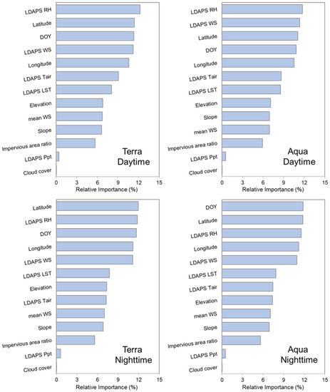
Figure 10.
Relative variable importance calculated from the LightGBM model for four MODIS view times. Relative variable importance was normalized by sum to 100%.
Under the cloudy conditions, we further investigated the impact of using the in situ cloudy-sky LST and cloud cover data in the LightGBM model by selectively excluding them (Table 3). Comparing the proposed model and two scenarios (i.e., scenario 1 and scenario 2) for clear-sky LST, they showed comparable performance, having slightly different R2 (~0.02) and RMSE (~0.02 °C) for all MODIS view times.
Table 3.
LOSOCV results of the proposed LightGBM and two scenario models (i.e., scenario 1 and scenario 2) for clear and cloudy-sky LSTs.
For cloudy-sky LST, however, the three models showed a noticeable difference in the accuracy metrics. Among the three models (i.e., the proposed model, scenario 1, and scenario 2), scenario 1 had the lowest R2 and highest RMSE for each MODIS view time, showing a warm bias ≥1 °C during the daytime and cold bias ≤−1 °C at nighttime. Scenario 2 yielded better LST estimation accuracy metrics under the cloud than scenario 1, which implies that it is beneficial to learn the LST information under the cloud from in situ observations for all-sky LST reconstruction. Compared to scenario 1, scenario 2 had a smaller bias, but still greater than 1 °C, except for Terra daytime. The warm bias during the daytime and the cold bias at nighttime in both scenarios 1 and 2 are due to the cloud effects on LST, with clouds cooling the LST during the daytime by reducing downwelling shortwave radiation and warming the LST at nighttime by increasing downwelling longwave radiation [22,23]. Although both MODIS LST and in situ cloudy-sky LST were used to train the model, the majority of training samples were clear-sky MODIS LST, which may have limited the model’s learning of cloudy-sky LST characteristics. In comparison to the two scenarios, the proposed model had the highest accuracy metrics with a much lower bias. These results demonstrate that the binary cloud cover input data adequately reflected the cloud effects considering the heterogeneity of the relationship between LST and other input variables under both clear and cloudy skies.
5.3. Spatial Distribution Assessment of All-Sky LSTs
Both LDAPS and LightGBM had a similar dynamic range of LST during the daytime, whereas LDAPS showed significantly wider nighttime LST ranges than LightGBM (Figure 7 and Figure 8). Under clear-sky conditions, LDAPS had a higher LST range than MODIS during both the daytime and nighttime. In addition, the comparison between the LDAPS LST and 22 in situ observations (Figure S3) revealed that the LDAPS had a warm bias in cloudy-sky conditions as well as in clear skies at nighttime, but LightGBM did not show such a bias (see Table 2). Moreover, the cloud makes LST cooler during the daytime and warmer during the nighttime. That is, LDAPS had a higher LST than MODIS under clear skies during the daytime, but it was smoothed by the cooling effect of the clouds, which resulted in similar LST ranges for both LDAPS and LightGBM. However, due to the warm bias of LDAPS under both clear and cloudy skies and the warming effect of clouds at night, LDAPS has a wider LST range than LightGBM.
The daytime and nighttime LSTs of LDAPS and LightGBM over the forest areas were relatively lower than those of the other land covers because forests contain various types of vegetation capable of photosynthesis and transpiration that help reduce the heat over the regions [62,63]. Meanwhile, the built-up areas had a higher LST than other land covers due to the huge amount of impervious surfaces [5,64]. These LST spatial distributions are coincident with the results of Yoo et al. (2020) [15]. Compared to LDAPS, LightGBM produced LST spatial distribution maps reflecting the spatial variation of LST according to the land cover and topography in South Korea. These spatial pattern differences were clearly seen in the metropolitan areas (boxes 1 and 2 in Figure 7 and Figure 8). LDAPS resulted in clustered hotspots that did not reflect the complex urban environment, whereas LightGBM not only yielded a higher LST in cities than their surrounding areas but also showed the spatial variability of LST within the cities. The LightGBM successfully reconstructed the all-sky MODIS LST (Figure 9), showing spatial patterns consistent with the original MODIS LST. These results indicate that the missing MODIS LST, mainly due to clouds, can be effectively filled seamlessly through the proposed reconstruction model.
5.4. Novelty and Limitations
Most previous LST gap-filling studies applied the relationship between the clear-sky LST and input variables to fill the missing MODIS LST by cloud. To consider the cloud effects on LST, this study used in situ LST measurements under cloud and cloud cover data along with high-resolution LDAPS meteorological data based on the LightGBM machine learning model. The proposed strategy in this study showed much higher cloudy-sky LST estimation accuracy metrics with RMSE of 2.41–3.00 °C during the daytime and 1.31–1.37 °C at nighttime than the approach proposed by Yoo et al. (2020), which is the same as scenario 2 in this study [15]. In addition, all-sky 1 km MODIS-like LST can be produced near real-time since this study used the analysis data of the operational LDAPS model. Thus, the generated all-sky LST data can be used for practical purposes such as initializing numerical weather forecasting models or assisting in emergency planning.
However, the proposed approach in this study has some limitations. Firstly, since LDAPS produces meteorological data at 3-h intervals, we linearly interpolated them for each MODIS view time and then used them as input data. Because LST has a relatively high diurnal variation, especially during the daytime, the time difference between LDAPS production and MODIS observation can introduce potential uncertainty in the LST reconstruction process. It is expected that the accuracy of LST reconstruction could be further improved when numerical model data with an hour interval or higher temporal resolution are used. Another limitation is the insufficient in situ observations, especially in urban areas where MODIS LST has relatively high uncertainty. Since the all-sky LST spatial distributions of LDAPS and LightGBM were qualitatively compared in two metropolitan cities in South Korea, additional quantitative validation across multiple cities is necessary using in situ observations.
6. Conclusions
This study developed an all-sky 1 km MODIS LST reconstruction model based on LightGBM to fill missing MODIS LST caused mainly by clouds in South Korea during summer seasons. The analysis data of LDAPS, seven auxiliary variables, and binary MODIS cloud cover were used as input variables, while MODIS LST and bias-corrected in situ cloudy-sky LST were used as dependent variables together. The RDCV and SPCV using MODIS LST showed that the proposed model produced a better performance than LDAPS, with an R2~0.9 and RMSE ≤ 1.4 °C and 0.6 °C during the daytime and nighttime, respectively. We evaluated the proposed model under cloudy conditions through LOSOCV using in situ data from 22 weather stations. Under cloudy conditions, LDAPS had an R2 of 0.54–0.59 and RMSE of 2.84–3.34 °C during the daytime, and an R2 of 0.72–0.75 and RMSE of 1.96–2.21 °C at nighttime. The proposed model had an R2 comparable to LDAPS, but it had a lower RMSE of 2.41–3.00 °C during the daytime and 1.31–1.36 °C at nighttime. These results revealed that the proposed model successfully reconstructed the all-sky 1 km MODIS LST. The model performance was improved by incorporating the in situ cloudy-sky LST and MODIS cloud cover data, which adequately reflected the cloud effect on LST.
In this study, instantaneous cloud information was used to reconstruct the all-sky 1 km MODIS LST. In the future, if the temporal variations of cloud-covered conditions such as cumulative incoming solar radiations suggested by Zhao and Duan (2020) are considered using geostationary satellite data, the all-sky MODIS LST reconstruction can be further improved [61]. Although this study used the LDAPS model available for South Korea, we believe that the proposed model could be effectively applied in other countries using WRF or other high-resolution numerical models for all-sky MODIS LST reconstruction.
Supplementary Materials
The following supporting information can be downloaded at: https://www.mdpi.com/article/10.3390/rs14081815/s1, Figure S1: Time-series of the estimated LST by LDAPS and LightGBM models, and bias-corrected in situ LST at station 8 for four MODIS view times (i.e., Terra and Aqua for daytime and nighttime) in August 2013. Figure S2: Temporal R2 between clear-sky LSTs observed in 22 ASOS at Terra and Aqua daytime and nighttime in June–August from 2013 to 2020. Figure S3: The bias of the LDAPS through 22 bias-corrected in situ observations from June to August from 2013 to 2020 at each MODIS view time.
Author Contributions
Conceptualization, D.C. and J.I.; methodology, D.C., D.B., C.Y. and J.I.; software, D.C.; validation, D.C.; formal analysis, D.C., D.B. and C.Y.; investigation, D.C., D.B., C.Y., Y.L. and S.L.; resources, D.C. and C.Y.; writing original draft preparation, D.C.; writing review and editing, D.B., C.Y., J.I., Y.L. and S.L.; visualization, D.C.; supervision, J.I.; project administration, J.I.; funding acquisition, J.I. and C.Y. All authors have read and agreed to the published version of the manuscript.
Funding
This research was supported by the Korea Meteorological Administration Research and Development Program under Grant KMIPA 2017–7010, the National Research Foundation of Korea (NRF) (NRF-2021R1A2C2008561), and the Korea Environment Industry & Technology Institute (KEITI) through the Digital Infrastructure Building Project for Monitoring, Surveying and Evaluating the Environmental Health, funded by the Korea Ministry of Environment (MOE) (2021003330001(NTIS: 1485017948)).
Data Availability Statement
The data and code used in this study are available upon request to the corresponding author. MODIS LST and landcover data (i.e., MOD11A1, MYD11A1, and MCD12Q1) were downloaded from Earthdata Search (https://search.earthdata.nasa.gov/search; assessed on 1 August 2021). Shuttle Radar Topography Mission (SRTM) Digital Elevation Model (DEM) was downloaded from the web page of the United States Geological Survey (USGS) (https://earthexplorer.usgs.gov; assessed on 1 August 2021). The Global Human Settlement (GHS) built-up dataset was downloaded from the European Commission’s Joint Research Centre (https://ghsl.jrc.ec.europa.eu/ghs_bu2019.php; assessed on 1 August 2021).
Conflicts of Interest
The authors declare no conflict of interest.
References
- Tomlinson, C.J.; Chapman, L.; Thornes, J.E.; Baker, C. Remote sensing land surface temperature for meteorology and climatology: A review. Meteorol. Appl. 2011, 18, 296–306. [Google Scholar] [CrossRef] [Green Version]
- Li, Z.-L.; Tang, B.-H.; Wu, H.; Ren, H.; Yan, G.; Wan, Z.; Trigo, I.F.; Sobrino, J.A. Satellite-derived land surface temperature: Current status and perspectives. Remote Sens. Environ. 2013, 131, 14–37. [Google Scholar] [CrossRef] [Green Version]
- Matuszko, D. Influence of the extent and genera of cloud cover on solar radiation intensity. Int. J. Climatol. 2012, 32, 2403–2414. [Google Scholar] [CrossRef]
- Wang, L.; Koike, T.; Yang, K.; Yeh, P.J.-F. Assessment of a distributed biosphere hydrological model against streamflow and MODIS land surface temperature in the upper Tone River Basin. J. Hydrol. 2009, 377, 21–34. [Google Scholar] [CrossRef]
- Yoo, C.; Im, J.; Park, S.; Quackenbush, L.J. Estimation of daily maximum and minimum air temperatures in urban landscapes using MODIS time series satellite data. ISPRS J. Photogramm. Remote Sens. 2018, 137, 149–162. [Google Scholar] [CrossRef]
- Ghazaryan, G.; Dubovyk, O.; Graw, V.; Kussul, N.; Schellberg, J. Local-scale agricultural drought monitoring with satellite-based multi-sensor time-series. GIScience Remote Sens. 2020, 57, 704–718. [Google Scholar] [CrossRef]
- Khan, M.S.; Baik, J.; Choi, M. A physical-based two-source evapotranspiration model with Monin–Obukhov similarity theory. GIScience Remote Sens. 2021, 58, 88–119. [Google Scholar] [CrossRef]
- Sabatini, F. Setting up and managing automatic weather stations for remote sites monitoring: From Niger to Nepal. In Renewing Local Planning to Face Climate Change in the Tropics; Springer: Cham, Switzerland, 2017; pp. 21–39. [Google Scholar]
- Freitas, S.C.; Trigo, I.F.; Macedo, J.; Barroso, C.; Silva, R.; Perdigão, R. Land surface temperature from multiple geostationary satellites. Int. J. Remote Sens. 2013, 34, 3051–3068. [Google Scholar] [CrossRef]
- Kalma, J.D.; McVicar, T.R.; McCabe, M.F. Estimating land surface evaporation: A review of methods using remotely sensed surface temperature data. Surv. Geophys. 2008, 29, 421–469. [Google Scholar] [CrossRef]
- Tran, D.X.; Pla, F.; Latorre-Carmona, P.; Myint, S.W.; Caetano, M.; Kieu, H.V. Characterizing the relationship between land use land cover change and land surface temperature. ISPRS J. Photogramm. Remote Sens. 2017, 124, 119–132. [Google Scholar] [CrossRef] [Green Version]
- Elmes, A.; Healy, M.; Geron, N.; Andrews, M.; Rogan, J.; Martin, D.; Sangermano, F.; Williams, C.; Weil, B. Mapping spatiotemporal variability of the urban heat island across an urban gradient in Worcester, Massachusetts using in-situ Thermochrons and Landsat-8 Thermal Infrared Sensor (TIRS) data. GIScience Remote Sens. 2020, 57, 845–864. [Google Scholar] [CrossRef]
- Mohammad, P.; Goswami, A. Quantifying diurnal and seasonal variation of surface urban heat island intensity and its associated determinants across different climatic zones over Indian cities. GIScience Remote Sens. 2021, 58, 955–981. [Google Scholar] [CrossRef]
- Gao, Z.; Hou, Y.; Zaitchik, B.F.; Chen, Y.; Chen, W. A Two-Step Integrated MLP-GTWR Method to Estimate 1 km Land Surface Temperature with Complete Spatial Coverage in Humid, Cloudy Regions. Remote Sens. 2021, 13, 971. [Google Scholar] [CrossRef]
- Yoo, C.; Im, J.; Cho, D.; Yokoya, N.; Xia, J.; Bechtel, B. Estimation of all-weather 1 km MODIS land surface temperature for humid summer days. Remote Sens. 2020, 12, 1398. [Google Scholar] [CrossRef]
- Xian, G.; Shi, H.; Auch, R.; Gallo, K.; Zhou, Q.; Wu, Z.; Kolian, M. The effects of urban land cover dynamics on urban heat Island intensity and temporal trends. GIScience Remote Sens. 2021, 58, 501–515. [Google Scholar] [CrossRef]
- Cho, D.; Yoo, C.; Im, J.; Lee, Y.; Lee, J. Improvement of spatial interpolation accuracy of daily maximum air temperature in urban areas using a stacking ensemble technique. GIScience Remote Sens. 2020, 57, 633–649. [Google Scholar] [CrossRef]
- Kang, J.; Tan, J.; Jin, R.; Li, X.; Zhang, Y. Reconstruction of MODIS land surface temperature products based on multi-temporal information. Remote Sens. 2018, 10, 1112. [Google Scholar] [CrossRef] [Green Version]
- Li, X.; Zhou, Y.; Asrar, G.R.; Zhu, Z. Creating a seamless 1 km resolution daily land surface temperature dataset for urban and surrounding areas in the conterminous United States. Remote Sens. Environ. 2018, 206, 84–97. [Google Scholar] [CrossRef]
- Pede, T.; Mountrakis, G. An empirical comparison of interpolation methods for MODIS 8-day land surface temperature composites across the conterminous Unites States. ISPRS J. Photogramm. Remote Sens. 2018, 142, 137–150. [Google Scholar] [CrossRef]
- Zhang, T.; Zhou, Y.; Zhu, Z.; Li, X.; Asrar, G.R. A global seamless 1 km resolution daily land surface temperature dataset (2003–2020). Earth Syst. Sci. Data Discuss. 2021, 14, 651–664. [Google Scholar] [CrossRef]
- Dai, A.; Trenberth, K.E.; Karl, T.R. Effects of clouds, soil moisture, precipitation, and water vapor on diurnal temperature range. J. Clim. 1999, 12, 2451–2473. [Google Scholar] [CrossRef]
- Zhang, H.; Zhang, F.; Zhang, G.; He, X.; Tian, L. Evaluation of cloud effects on air temperature estimation using MODIS LST based on ground measurements over the Tibetan Plateau. Atmos. Chem. Phys. 2016, 16, 13681–13696. [Google Scholar] [CrossRef] [Green Version]
- Lu, L.; Venus, V.; Skidmore, A.; Wang, T.; Luo, G. Estimating land-surface temperature under clouds using MSG/SEVIRI observations. Int. J. Appl. Earth Obs. Geoinf. 2011, 13, 265–276. [Google Scholar] [CrossRef]
- Yu, W.; Ma, M.; Wang, X.; Tan, J. Estimating the land-surface temperature of pixels covered by clouds in MODIS products. J. Appl. Remote Sens. 2014, 8, 083525. [Google Scholar] [CrossRef]
- Zeng, C.; Long, D.; Shen, H.; Wu, P.; Cui, Y.; Hong, Y. A two-step framework for reconstructing remotely sensed land surface temperatures contaminated by cloud. ISPRS J. Photogramm. Remote Sens. 2018, 141, 30–45. [Google Scholar] [CrossRef]
- Jia, A.; Ma, H.; Liang, S.; Wang, D. Cloudy-sky land surface temperature from VIIRS and MODIS satellite data using a surface energy balance-based method. Remote Sens. Environ. 2021, 263, 112566. [Google Scholar] [CrossRef]
- Yang, G.; Sun, W.; Shen, H.; Meng, X.; Li, J. An integrated method for reconstructing daily MODIS land surface temperature data. IEEE J. Sel. Top. Appl. Earth Obs. Remote Sens. 2019, 12, 1026–1040. [Google Scholar] [CrossRef]
- Holmes, T.; De Jeu, R.; Owe, M.; Dolman, A. Land surface temperature from Ka band (37 GHz) passive microwave observations. J. Geophys. Res. Atmos. 2009, 114, D4. [Google Scholar] [CrossRef] [Green Version]
- Mo, Y.; Xu, Y.; Chen, H.; Zhu, S. A Review of Reconstructing Remotely Sensed Land Surface Temperature under Cloudy Conditions. Remote Sens. 2021, 13, 2838. [Google Scholar] [CrossRef]
- Royer, A.; Poirier, S. Surface temperature spatial and temporal variations in North America from homogenized satellite SMMR–SSM/I microwave measurements and reanalysis for 1979–2008. J. Geophys. Res. Atmos. 2010, 115, D08110. [Google Scholar] [CrossRef]
- Xu, S.; Cheng, J. A new land surface temperature fusion strategy based on cumulative distribution function matching and multiresolution Kalman filtering. Remote Sens. Environ. 2021, 254, 112256. [Google Scholar] [CrossRef]
- Zhang, Q.; Wang, N.; Cheng, J.; Xu, S. A stepwise downscaling method for generating high-resolution land surface temperature from AMSR-E data. IEEE J. Sel. Top. Appl. Earth Obs. Remote Sens. 2020, 13, 5669–5681. [Google Scholar] [CrossRef]
- Prigent, C.; Rossow, W.B.; Matthews, E.; Marticorena, B. Microwave radiometric signatures of different surface types in deserts. J. Geophys. Res. Atmos. 1999, 104, 12147–12158. [Google Scholar] [CrossRef] [Green Version]
- Long, D.; Yan, L.; Bai, L.; Zhang, C.; Li, X.; Lei, H.; Yang, H.; Tian, F.; Zeng, C.; Meng, X. Generation of MODIS-like land surface temperatures under all-weather conditions based on a data fusion approach. Remote Sens. Environ. 2020, 246, 111863. [Google Scholar] [CrossRef]
- Tan, W.; Wei, C.; Lu, Y.; Xue, D. Reconstruction of All-Weather Daytime and Nighttime MODIS Aqua-Terra Land Surface Temperature Products Using an XGBoost Approach. Remote Sens. 2021, 13, 4723. [Google Scholar] [CrossRef]
- Li, B.; Liang, S.; Liu, X.; Ma, H.; Chen, Y.; Liang, T.; He, T. Estimation of all-sky 1 km land surface temperature over the conterminous United States. Remote Sens. Environ. 2021, 266, 112707. [Google Scholar] [CrossRef]
- Padhee, S.K.; Dutta, S. Spatiotemporal reconstruction of MODIS land surface temperature with the help of GLDAS product using kernel-based nonparametric data assimilation. J. Appl. Remote Sens. 2020, 14, 014520. [Google Scholar] [CrossRef]
- Zhang, X.; Zhou, J.; Liang, S.; Wang, D. A practical reanalysis data and thermal infrared remote sensing data merging (RTM) method for reconstruction of a 1-km all-weather land surface temperature. Remote Sens. Environ. 2021, 260, 112437. [Google Scholar] [CrossRef]
- Zhong, Y.; Meng, L.; Wei, Z.; Yang, J.; Song, W.; Basir, M. Retrieval of All-Weather 1 km Land Surface Temperature from Combined MODIS and AMSR2 Data over the Tibetan Plateau. Remote Sens. 2021, 13, 4574. [Google Scholar] [CrossRef]
- Wan, Z.; Dozier, J. A generalized split-window algorithm for retrieving land-surface temperature from space. IEEE Trans. Geosci. Remote Sens. 1996, 34, 892–905. [Google Scholar]
- Orr, A.; Phillips, T.; Webster, S.; Elvidge, A.; Weeks, M.; Hosking, S.; Turner, J. Met Office Unified Model high-resolution simulations of a strong wind event in Antarctica. Q. J. R. Meteorol. Soc. 2014, 140, 2287–2297. [Google Scholar] [CrossRef] [Green Version]
- Abbas, A.; He, Q.; Jin, L.; Li, J.; Salam, A.; Lu, B.; Yasheng, Y. Spatio-Temporal Changes of Land Surface Temperature and the Influencing Factors in the Tarim Basin, Northwest China. Remote Sens. 2021, 13, 3792. [Google Scholar] [CrossRef]
- Peng, X.; Wu, W.; Zheng, Y.; Sun, J.; Hu, T.; Wang, P. Correlation analysis of land surface temperature and topographic elements in Hangzhou, China. Sci. Rep. 2020, 10, 10451. [Google Scholar] [CrossRef]
- Stroppiana, D.; Antoninetti, M.; Brivio, P.A. Seasonality of MODIS LST over Southern Italy and correlation with land cover, topography and solar radiation. Eur. J. Remote Sens. 2014, 47, 133–152. [Google Scholar] [CrossRef]
- Buciluǎ, C.; Caruana, R.; Niculescu-Mizil, A. Model compression. In Proceedings of the 12th ACM SIGKDD International Conference on Knowledge Discovery and Data Mining, Philadelphia, PA, USA, 20–23 August 2006; pp. 535–541. [Google Scholar]
- Ke, G.; Meng, Q.; Finley, T.; Wang, T.; Chen, W.; Ma, W.; Ye, Q.; Liu, T.-Y. Lightgbm: A highly efficient gradient boosting decision tree. Adv. Neural Inf. Processing Syst. 2017, 30, 3146–3154. [Google Scholar]
- Pham, T.D.; Yokoya, N.; Nguyen, T.T.T.; Le, N.N.; Ha, N.T.; Xia, J.; Takeuchi, W.; Pham, T.D. Improvement of mangrove soil carbon stocks estimation in North Vietnam using Sentinel-2 data and machine learning approach. GIScience Remote Sens. 2021, 58, 68–87. [Google Scholar] [CrossRef]
- Al Daoud, E. Comparison between XGBoost, LightGBM and CatBoost using a home credit dataset. Int. J. Comput. Inf. Eng. 2019, 13, 6–10. [Google Scholar]
- Candido, C.; Blanco, A.; Medina, J.; Gubatanga, E.; Santos, A.; Ana, R.S.; Reyes, R. Improving the consistency of multi-temporal land cover mapping of Laguna lake watershed using light gradient boosting machine (LightGBM) approach, change detection analysis, and Markov chain. Remote Sens. Appl. Soc. Environ. 2021, 23, 100565. [Google Scholar] [CrossRef]
- Huang, S.; Wang, C.; Ding, B.; Chaudhuri, S. Efficient identification of approximate best configuration of training in large datasets. In Proceedings of the AAAI Conference on Artificial Intelligence, Honolulu, HI, USA, 27 January–1 February 2019; pp. 3862–3869. [Google Scholar]
- Liu, X.; Duan, H.; Huang, W.; Guo, R.; Duan, B. Classified Early Warning and Forecast of Severe Convective Weather Based on LightGBM Algorithm. Atmos. Clim. Sci. 2021, 11, 284–301. [Google Scholar] [CrossRef]
- Kang, Y.; Kim, M.; Kang, E.; Cho, D.; Im, J. Improved retrievals of aerosol optical depth and fine mode fraction from GOCI geostationary satellite data using machine learning over East Asia. ISPRS J. Photogramm. Remote Sens. 2022, 183, 253–268. [Google Scholar] [CrossRef]
- Reitz, O.; Graf, A.; Schmidt, M.; Ketzler, G.; Leuchner, M. Upscaling net ecosystem exchange over heterogeneous landscapes with machine learning. J. Geophys. Res. Biogeosci. 2021, 126, e2020JG005814. [Google Scholar] [CrossRef]
- Aires, F.; Prigent, C.; Rossow, W. Temporal interpolation of global surface skin temperature diurnal cycle over land under clear and cloudy conditions. J. Geophys. Res. Atmos. 2004, 109, D4. [Google Scholar] [CrossRef]
- Yang, Y.Z.; Cai, W.H.; Yang, J. Evaluation of MODIS land surface temperature data to estimate near-surface air temperature in Northeast China. Remote Sens. 2017, 9, 410. [Google Scholar] [CrossRef] [Green Version]
- Cho, D.; Yoo, C.; Im, J.; Cha, D.H. Comparative assessment of various machine learning-based bias correction methods for numerical weather prediction model forecasts of extreme air temperatures in urban areas. Earth Space Sci. 2020, 7, e2019EA000740. [Google Scholar] [CrossRef] [Green Version]
- Cho, D.; Yoo, C.; Son, B.; Im, J.; Yoon, D.; Cha, D.-H. A novel ensemble learning for post-processing of NWP Model’s next-day maximum air temperature forecast in summer using deep learning and statistical approaches. Weather Clim. Extrem. 2022, 35, 100410. [Google Scholar] [CrossRef]
- Webster, S.; Brown, A.; Cameron, D.; Jones, C. Improvements to the representation of orography in the Met Office Unified Model. Q. J. R. Meteorol. Soc. A J. Atmos. Sci. Appl. Meteorol. Phys. Oceanogr. 2003, 129, 1989–2010. [Google Scholar] [CrossRef]
- Guo, D.; Wang, C.; Zang, S.; Hua, J.; Lv, Z.; Lin, Y. Gap-Filling of 8-Day Terra MODIS Daytime Land Surface Temperature in High-Latitude Cold Region with Generalized Additive Models (GAM). Remote Sens. 2021, 13, 3667. [Google Scholar] [CrossRef]
- Zhao, W.; Duan, S.-B. Reconstruction of daytime land surface temperatures under cloud-covered conditions using integrated MODIS/Terra land products and MSG geostationary satellite data. Remote Sens. Environ. 2020, 247, 111931. [Google Scholar] [CrossRef]
- Hua, A.K.; Ping, O.W. The influence of land-use/land-cover changes on land surface temperature: A case study of Kuala Lumpur metropolitan city. Eur. J. Remote Sens. 2018, 51, 1049–1069. [Google Scholar] [CrossRef] [Green Version]
- Wickham, J.D.; Wade, T.G.; Riitters, K.H. Comparison of cropland and forest surface temperatures across the conterminous United States. Agric. For. Meteorol. 2012, 166, 137–143. [Google Scholar] [CrossRef]
- Xu, H. Analysis of impervious surface and its impact on urban heat environment using the normalized difference impervious surface index (NDISI). Photogramm. Eng. Remote Sens. 2010, 76, 557–565. [Google Scholar] [CrossRef]
Publisher’s Note: MDPI stays neutral with regard to jurisdictional claims in published maps and institutional affiliations. |
© 2022 by the authors. Licensee MDPI, Basel, Switzerland. This article is an open access article distributed under the terms and conditions of the Creative Commons Attribution (CC BY) license (https://creativecommons.org/licenses/by/4.0/).