Article

Geophysical Study of the Diendorf-Boskovice Fault System (Austria)

1
Dipartimento di Scienze della Terra, dell’Ambiente e delle Risorse, University of Naples Federico II, Via Vicinale Cupa Cintia 21, 80126 Naples, Italy
2
Geological Survey of Austria, Neulinggasse 38, 1080 Vienna, Austria
3
Dipartimento di Ingegneria Civile, Ambientale e Architettura, University of Cagliari, Via Marengo 2, 09123 Cagliari, Italy
*
Author to whom correspondence should be addressed.
Remote Sens. 2022, 14(8), 1807; https://doi.org/10.3390/rs14081807
Submission received: 26 February 2022 / Revised: 4 April 2022 / Accepted: 6 April 2022 / Published: 8 April 2022

Abstract

:
We describe here the results of the characterization of subsurface structures in an area of the south-eastern edge of the Bohemian Massif, in Austria by high-resolution geophysical survey techniques and advanced analysis methods of potential fields. The employed methods included potential field multiscale techniques for source-edge location and characterization of sources at depth. Our results confirmed the presence of already known structures: the location of the Diendorf Fault and the Moldanubian Shearzone are clearly recognized in the data at the same location as on the geological maps, even where the Diendorf fault is covered with sediments of the Molasse Basin. In addition, we detected several geological contacts between different rock types in the Bohemian Massif west of the Diendorf Fault. From our results, we were also able to quickly identify and image, without a priori information, previously unknown structures, such as faults with-depth-to-the top of about 500 m and magmatic intrusions about 400 m deep.

1. Introduction

Geophysical high-resolution techniques are important methods to characterize systems of faults in tectonically complex regions. Often, only limited portions of faults are exposed at the surface, due to the combined result of erosion and tectonic rock exhumation. Thus, important details of the faults are hidden beneath basins. This can make the signature of faulting difficult to read. Geophysical active methods and passive methods can yield quick and effective information on the subsoil characteristics and/or rupture planes, thus highlighting interesting areas to be possibly studied in detail. Among a wide range of methods used for geological interpretation, airborne magnetic and gravimetric surveys, along with electromagnetic and radiometric investigations, have a central role for the characterization of the subsurface and to constrain 2D and 3D modeling of geological structures (e.g., [1,2,3,4,5,6,7,8]).
The acquisition of appropriately spaced data and the subsequent processing of the same yield maps of anomalies of different nature in connection with the different physical properties of the rocks—the density in the case of the gravimetric method, the magnetization in the magnetic one, the resistivity (or conductivity) in the electromagnetic method and the natural radioactivity in the radiometric one.
The main advantages of aerial surveys are the speed of data acquisition and the completeness of coverage of the surveys. In general, aerial surveys play a fundamental role in the reconnaissance phase, which is often the initial phase of any exploration, be it mining, oil, environmental, or geological. However, some modern airborne systems offer such a high resolution that they manage to acquire at small distances from the ground level (100–200 m distance for helicopters, 40–50 m for drones), which can also be applied in the phases of subsequent studies dedicated to the geophysical/geological characterization of the sites.
The present work describes the study and characterization of subsurface structures (deeper than 500 m) in an area of the southeastern edge of the Bohemian Massif in Austria (Figure 1), using high-resolution geophysical survey techniques and advanced analysis methods of potential fields. The complicated geodynamic evolution of this suture area, dated from the Variscian period and resulted in a complex area characterized by numerous subunits of different geological and geophysical properties, as well as a widely dissected topographic profile [9]. The main Paleozoic geological structure, the Diendorf-Boskovice-Čebín fault system, the extraordinary abundance of plutonic basement rocks from the Cadomian age and the magmatic intrusions of the same age represent the main characteristics of this area [10].
Thanks to the use of geophysical methodologies applied to potential field data, it is possible to characterize structures such as faults and intrusive bodies of different extent and depth, locating them both in plan thanks to edge analysis methods, and in depth, thanks to imaging methods. Even though the tectonic structures in this area are mapped well in a map view, their extent in depth is not well-known. The complex multi-phased deformation history of the structures prevents a simple extrapolation from surface observations into the depth.
The results of this work aim at broadening the geological knowledge of the area by corroborating the presence of already known structures but also by showing—quickly and without a priori information—how it was possible to circumscribe and detail previously unknown structures.

2. Geological and Geophysical Background

2.1. Major Geological Structures in the Study Area

The most prominent geological structure in the study area is the Diendorf-Boskovice Fault System (DBFS), a c. 200 km long, approximately NE-SW trending fault system that forms the eastern margin of the Austrian part of the Bohemian Massif (Figure 1). It extends from south of the Danube via the city of Krems (AT) towards the city of Brno (CZ), where it is supposed to be kinematically linked to the Boskovice Furrow. It includes the Diendorf and Boskovice faults, both showing a long-lasting and multiphase history from Variscan times. In addition, the Waitzendorf Fault (WF) is part of the fault system and strikes NNE-SSW [9]. Proofs of NE-SW-striking left-lateral strike-slip partly ductile, mylonitic shear zones during Upper Carboniferous and Permian times are observed along the Diendorf Fault System (DFS). Several studies show not only insights of continuous transtensional left-lateral strike-slip faulting during Miocene, but also recent tectonic activity [9,11]. Total sinistral displacement along the Diendorf Fault is estimated to be between 25 km, derived from offset of granitic blocks [12], and about 40 km, derived from offset of magnetic anomalies [13]. Westward, the Freyenstein Fault System (FFS) extends over 45 km and represents a ductile shear zone overprinted by a brittle fault located at the eastern edge of the South Bohemian Batholith towards the Moldanubian nappes [14].
First systematic gravity measurements along the DFS [13] recognized an elongated, NE-SW trending local minimum from the River Danube up to the border of Austria with the Czech Republic, which follows the trend of the DFS. Additional magnetic measurements along two profiles proved the existence of anomalies at the same location as the gravity minimum. These airborne campaigns were accompanied by ground measurements, mostly geoelectrical and seismic profiles [15,16,17,18]. The ground profiles suggest that the anomalies in the Molasse Basin are mostly granitic blocks that are uplifted along minor N-S striking faults between the DFS and the WF.
The second important geological structure is the Molanubian Shearzone (MSZ in Figure 1), a Variscan E-dipping shearzone, where the Moldavian Superunit is thrusted over the Moravian Superunit. In its southern part, the structure runs N-S, creating the geomorphic eastern margin of the Horn Basin, then bending by 90° into a E-W trend along the northern margin of the Horn Basin, and then finally bending again into a NE-SW striking [19]. The MSZ, together with the WF and the DFS, bound the so-called Thaya tectonicwindow or dome, where the metamorphic orthogneissic rocks of the Moravian Superunit are exposed [19,20].
Figure 1. The study area: (a) DTM model (SRTM 1 arc model [21]); black lines show the main geological structures of the region, (b) geological sketch map (modified after [22]). MSZ: Moldanubian Shearzone; DFS: Diendorf Fault System; WF: Waitzendorf Fault; FFS: Freyenstein Fault System.
Remotesensing 14 01807 g001
Between 1957 and 1978, the OMV company measured petrophysical parameters, such as vertical intensity (vertical component of total magnetic intensity) and magnetic susceptibility, on samples and drill-cores in the framework of hydrocarbon exploration in the study area. The documentation of those in situ magnetic results provided additional information to the aeromagnetic surveys carried out by the GBA in the early 1980s [23]. Another study of in situ measurements of rock densities and susceptibilities conducted in the eastern part of the Bohemian Massif was published 1985 and resulted in rock density and magnetic susceptibility maps [24].

2.2. Insight for Recent Tectonic Activity

The first suggestions that the DBFS might be a tectonically active fault system were based on extensive measurements of joints on both sides of the DFS [25]. The same main direction parallel to the DFS in both, crystalline rocks and loess deposits was observed, and it was concluded that the DFS must have been active after the loess deposition. Few earthquakes have been observed along the southern part of the DFS, whereas there are no earthquake records in the part north of the river Danube [26].
Repeated levelling measurements across the Boskovice Furrow show recent tectonic activity at its eastern margin, suggesting that the Boskovice Fault, the marginal fault of the Boskovice Furrow, is indeed active [10,27,28,29]. In addition, geomorphologic assessment of the fault scarps forming the margins of the Boskovice Furrow suggest that tectonic movement influences the courses of rivers into and out of the Boskovice Furrow [9]. Leichmann and Hejl [30] describe fluvial gravels und loess deposits offset by a NNW-SSE trending fault close to Brno.

3. Data and Methods

3.1. Datasets (Gravimetric, Magnetic, FDEM, Gamma-Ray)

The geophysical dataset used in this work includes land gravimetric data, acquired in the frame of several surveys, and airborne data acquired by five different helicopter-borne surveys (Figure 2a). The coordinates of datasets are in the “MGI-Austria-Lambert” reference system that is a projected reference coordinate system (CRS), used for representing Austrian data.

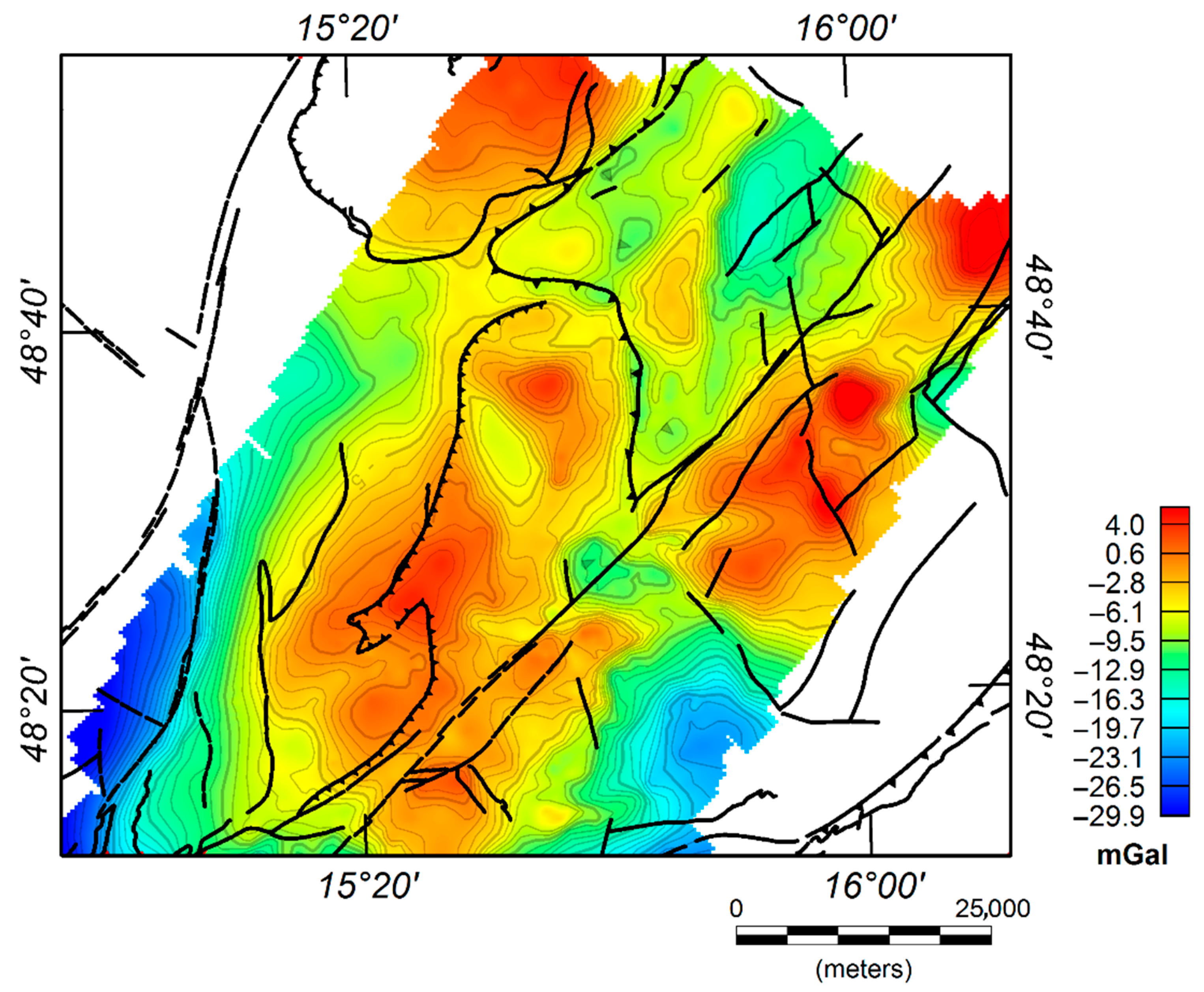
3.1.1. Gravimetric Data

Gravimetric data, unevenly distributed, have been acquired over the last 60 years by different institutions and cover a larger area with respect to airborne data. The different Bouguer gravity maps were brought together and homogenized by the Austrian Federal Office of Metrology and Surveying (BEV) to obtain a single Bouguer gravity map. To this end, all gravimetric data underwent a preliminary processing [31], including (1) calibration, (2) correction of wrong coordinates, and (3) mass correction.
  • Calibration. Due to the different institutions that conducted the acquisitions, the datum levels of the various data were different. After the appropriate modifications, each data was referred to the absolute gravimetric datum established by [32].
  • Correction of wrong coordinates. The low quality of some old topographic maps, from which the horizontal coordinates of measuring stations were obtained, caused systematic errors. To check these errors, the station heights were compared with those obtained by interpolating a high-resolution digital terrain model (with spacing 50 m). Wrong coordinates were corrected using recent topographic maps and using the digital land registry [28].
  • Mass correction. The gravitational effect of the topographic masses was calculated by applying an extremely accurate correction method: in the immediate vicinity of the stations (distance < 1200 m) the topography was approximated by bodies of arbitrary shape (polyhedral) [33], instead of flat-topped prisms. Considering the Earth’s curvature, all mass corrections were calculated in a spherical approximation with a radius of 167 km, assuming a density of 2670 kgm−3, a value very close to the density of the surface rocks of the investigated area. Rock densities measured in 1991 in situ and in drill cores in the study area within the Bohemian Massif area generally show a wide variation, depending not only on the type of rocks but also on the content of minerals. Nevertheless, they confirm this assumed average value of 2670 kgm−3 [34].
Moreover, for the first time, the Bouguer anomalies of Austria were calculated using an ellipsoidal height system. This allows exact estimates of the geophysical indirect effect (GIE) varying about 2 mGal in Austria [35]. Figure 3 shows the Bouguer map obtained by gridding the corrected data with Kriging at an interval of 360 m. It is characterized by several maxima mainly located in the central and eastern side of the surveyed area.

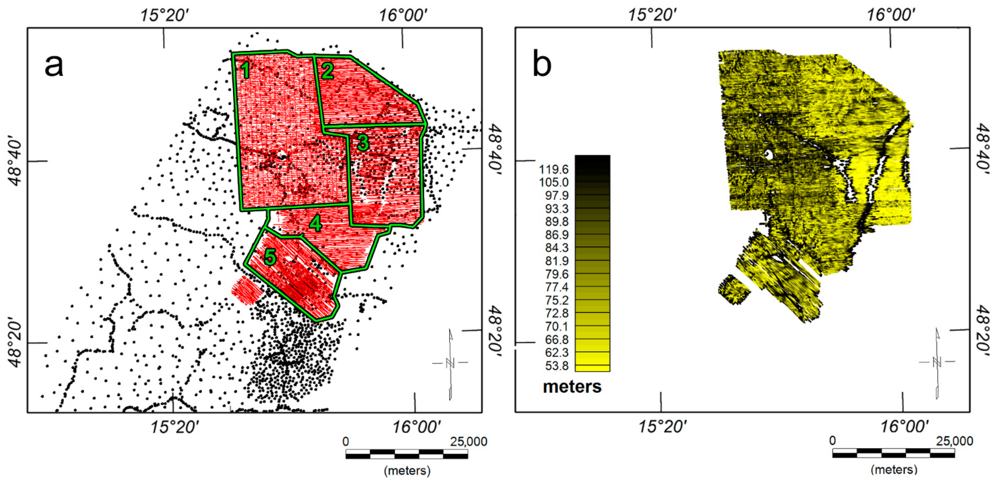
3.1.2. Airborne Data

The airborne surveys were carried out by the Geological Survey of Austria (GBA) [36] over a period of 14 years, between 1983 and 1997, in adjacent areas, numbered from 1 to 5 in Figure 2a and named Geras (1996 and 1997), Pulkau north (1995), Pulkau (1994), Kamptal-Ziersdorf (1983), and Kremser Bucht (1983), respectively. In all cases, aero-magnetic, aero-electromagnetic (AEM), and aero-radiometric data were collected simultaneously, using helicopter-towed geophysical equipment containing three different sensors. For all surveys, the average distance between flight lines was 200 m, while the clearance between the ground and the helicopter was mostly about 80 m (Figure 2b). However, some changes concerning data acquisition as the instrumentation was changed and improved several times over the years, as summarized in Table 1.
Vintage geophysical datasets are generally not as accurate as those collected and processed with modern equipment and software tools. More specifically, the position and height recording were quite imprecise in the 1980s and 1990s. The process of editing and correcting old data was not as standardized as now and the used software was written by GBA. Contemporary geological fault maps were used to support the results.
The data sets of each sub-area were processed by GBA following different specific procedures described below and were then merged into a single aeromagnetic, aero-electromagnetic, and aero-radiometric data set (Figure 4, Figure 5 and Figure 6).

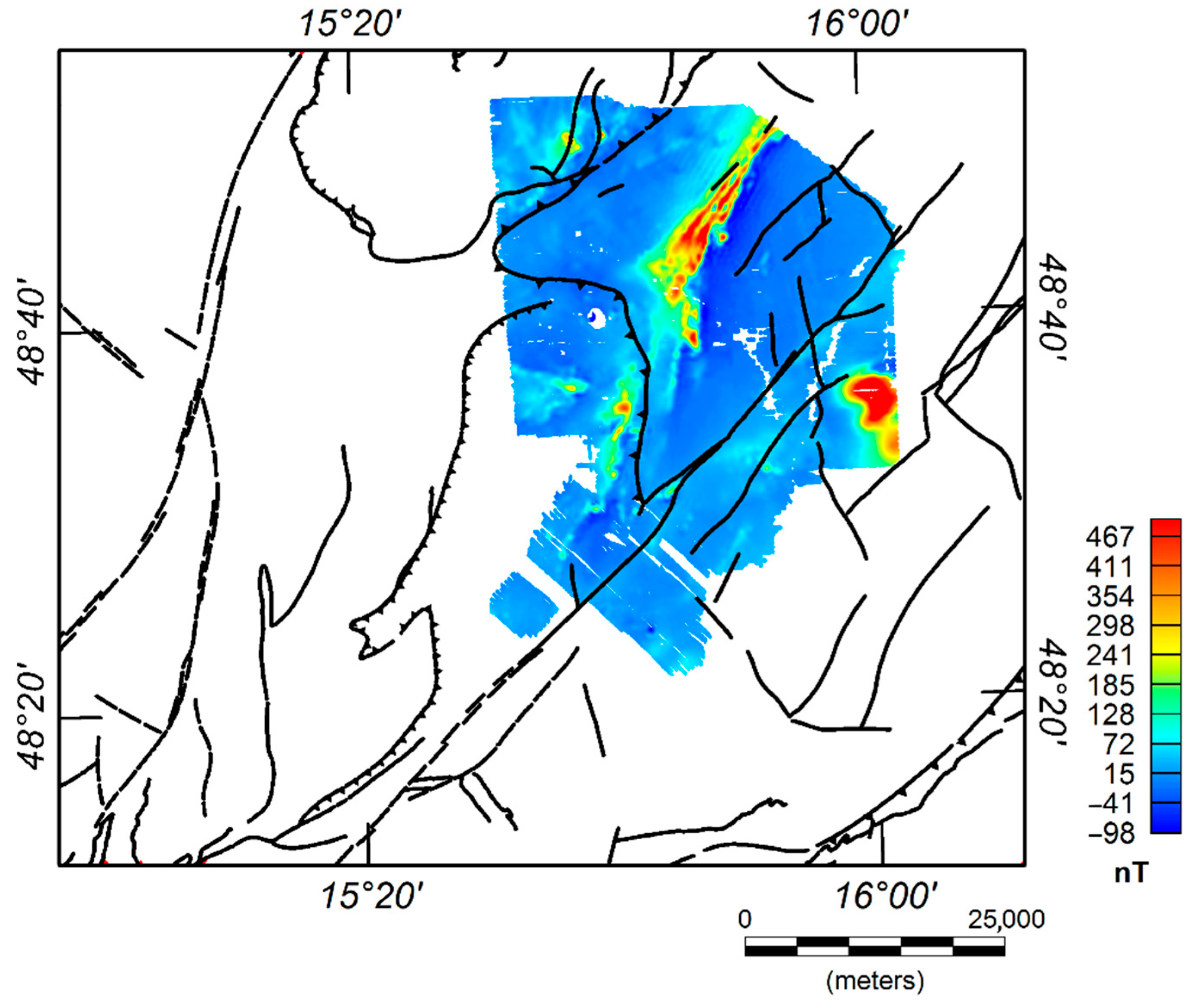
A—Aero-Magnetic Data

Airborne magnetic anomaly maps can provide important insights into the subsurface structure of complex areas characterized by mafic rocks because of their high magnetic response (e.g., [5,37]). In situ measurements carried out in 1991 in the Bohemian Massif show mainly susceptibility values between 0.1 and 0.2 × 10⁻³ (SI unit) [34]. However, a classification of rocks based solely on their susceptibility values is not possible due to the overlapping ranges of the measurement results. Helicopter-borne acquisition allows quick measurements in rugged and inaccessible regions and can provide a satisfactory sampling of the complex magnetic anomaly pattern that often characterizes tectonic areas.
Two different magnetometers were used within the period in which the surveys were carried out in the study area. A proton precision magnetometer (G-801/3) was used until 1994. Then the instrument was replaced with a more accurate cesium vapor magnetome-ter (Scrintrex CS-2), which was located inside the EM-bird. Both devices were carried 20–30 m below the helicopter. Further recording details, can be found in the survey-specific technical reports [15,16,17,18], provided by the GBA and available online. In 1998, the individual magnetic datasets were reprocessed and combined to a single map. This reprocessing step comprises the standard corrections on raw data including: (i) removal of spikes and gaps in the data; (ii) flight path check and repositioning, which consisted in the removal of wrong coordinates, correction of the GPS data, and check of the flight altitude; (iii) Earth’s magnetic field diurnal variation correction, which was performed using a local base station data; (iv) removal of the International Geomagnetic Reference Field (IGRF); (v) statistical leveling, consisting of minimization of the differences between the field values measured at the crossing points of flight lines and tie lines; (vi) reduction to the pole (RTP) using as average values of magnetic field direction for the whole dataset, inclination 65° and declination 5°.
After the data correction procedures, RTP aeromagnetic data were gridded to an interval of 100 m by using the Kriging algorithm. The obtained maps (Figure 4) are characterized by a few prominent anomalies (amplitude about 1000 nT) that align along NE–SW trends. Their interpretation is described in Section 4.

B—Aero-Electromagnetic Data

Regarding AEM data, the Austrian airborne system incorporates the frequency domain electromagnetic (FDEM) method. As mentioned, the main part of a frequency domain electromagnetic system consists of a bird containing several transmitting coils as well as receiving coils in different geometric arrangements (co-axial, co-planar loops). The transmitting coils generate an electromagnetic alternating field with certain frequencies (see Table 1). This primary field induces eddy currents in the conductive subsurface layers. These currents generate in turn a secondary magnetic field that induces a current in the receiver coils. Based on the amplitude and the phase shift of the secondary field relatively to the primary field, conclusions can be drawn on the electrical resistivity of the subsurface [38]. As reported in Table 1, the acquisitions were carried out over a period of several years, so the used frequencies vary for the five areas. The number of loop pairs and the loop configurations of the airborne EM-systems change depending on the survey period.
The exploration depth (the maximum depth to which a good electrical conductor in the underground can be detected) can be assumed to be 100–150 m [15,16,17,18]. In 1998, all the electromagnetic datasets acquired over the years in the five areas were reprocessed and homogenized. Figure 5 shows the homogeneous half-space of real resistivities obtained from the inversion of the apparent resistivity data. We discuss its correlation with geology in Section 5.

C—Aero-Radiometric Data

Airborne gamma-ray spectroscopy determines natural and artificial radioactivity, which depends on the content of radioactive minerals (containing potassium, uranium, and thorium) within the first decimeters of the subsurface. Igneous rocks show a general tendency of increasing radioelement concentrations with degree of magma differentiation, as clearly shown by mildly alkaline and peralkaline volcanics (e.g., [39]). Furthermore, felsic volcanic rocks often show very high radioelement concentrations compared to average crustal abundances.
The gamma-ray spectrometer consists of several sodium iodide crystals, which convert gamma radiation into flashes of light converted into an output voltage, which is proportional to the energy of the incident gamma-ray. Since the air layer between helicopter and ground absorbs gamma radiation (depending on the physical condition of the air), the exact flight altitude, air pressure, air temperature as well as air moisture should be considered when correcting survey data (as described below). Regarding the investigation depth, we note that when gamma rays pass through matter, they lose part of their energy through scattering and absorption. Therefore, most gamma-rays detected at airborne survey heights originate from the first 30 cm of the subsurface [38].
Two different gamma-ray spectrometers were used within the study area (Table 1). Geometrics GR-800B, used in the 1980s contains two sodium iodide crystals with a total volume of 33.6 L. The gamma-ray intensity of this device is sampled into 256 energy channels. Scintrex PGAM-1000 has the same specifications as Geometrics GR-800B but with the addition of an upward looking sodium iodide crystal (for radon correction). The total volume of this device is 37.7 L. The integration time of both devices was 1 s. All airborne gamma-ray data were processed by GBA through the following steps: (i) reduction of cosmic radiation, whose intensity mainly depends on the thickness of the atmosphere above the survey locations; (ii) reduction of the background, to remove the influence of the helicopter and the sensor material while the background of the helicopter is assumed to be a constant; (iii) reduction of the Compton effect due to the presence of anthropogenic radionuclides; (iv) removal of radiometric anomalies related to radon dispersed in the area; (v) height correction, removing the effects of the flight height change. The height variations represent the most significant perturbation to radiometric measurements from aircraft, as the gamma-ray intensity decreases rapidly with increasing flight height, due to the absorption of gamma-rays by the air [40]. Figure 6 shows the maps of thorium, potassium and uranium. Their pattern agrees with the nature of sediments and deposits of the area (see Figure 1). We remark that as the distribution of areo-radiometric gamma-ray data is connected to rather shallow sources, a comparison with gravity and magnetic anomalies and with their computed signals (i.e., EHD) is not always straightforward.

3.2. Methods

3.2.1. EHD

To identify the gravimetric lineaments of the study area, we performed a Multiscale Derivative Analysis (MDA) [41] of the Bouguer anomaly gravity field. MDA is based on the resolutive properties of the Enhanced Horizontal Derivative (EHD) [42,43,44]. The EHD is a high-resolution multiscale boundary estimator based on the horizontal derivative of a weighted sum of any-order derivative of the gravity or magnetic potential:
EHD ( x , y ) = ( ϕ x ) 2 + ( ϕ y ) 2 ,
where
ϕ ( x , y ) = w 0 f ( x , y ) + w 1 f ( 1 ) ( x , y ) + w 2 f ( 2 ) ( x , y ) + + w m f ( m ) ( x , y ) ,
and f ( m ) ( x , y ) is the p-order derivative of the potential and w0, …, wm are the set of weights that control the relative influence of the single terms in the summation. By adding higher-order derivative terms, a better detail of the shallower sources is obtained. The use of the highest order derivatives is in practice limited by the data-sampling step.
By this analysis, the source boundaries in the studied area are emphasized as the maxima of the EHD signal. As sources of different depth/extent generate effects at various scales, different images of the source edges can be obtained by appropriately choosing the first and last terms of the summation (2). The outcome of MDA consists of a combination of derivative terms which enhances the effects at a specific scale. The lower order terms represent deeper sources or larger scale effects; the highest order terms are suitable for small scale and shallow field components. A key feature of the MDA method is that it does not apply sharp component separation but enhances the contributions with a different resolution contained in the data.

3.2.2. Multi-Ridge Geometric Method

This method is built by joining extreme points of the analyzed field at different altitudes and uses a geometric criterion to find the structural index and vertical and horizontal source positions [45]. The extreme points represent the zeros (or maxima) of the field and its p-order spatial derivatives, calculated over a set of altitudes.
Multi-ridge analysis consists of two steps: (1) a set of ridges is constructed, and the position of the source is identified from the intersection point of the various ridges in the underground. In fact, thanks to the homogeneity law, the ridges of the vertical and horizontal derivatives of the field (i.e., the maxima lines) may be graphically extrapolated from the measurement plane to the source position. Thus, all maxima lines converge at the source depth and position; (2) one or more ridges are selected, and Euler deconvolution is applied to the field values along these ridges to estimate the structural index and/or the depth to the source.

3.2.3. DEXP

To study the geometry and depth extent of the faults and structures we performed a gravity multiscale analysis through the Depth from Extreme Points method (DEXP) [46,47], that is a fast technique for analysis of potential fields yielding a 3D image of the source distribution. The DEXP transformation is given by:
Ω ( r , z i ) = T ( r , z i ) | z i | N 2 . i = 1 , , L ,
where Ω ( r , z i ) is the DEXP-scaled field at the altitude zi, T ( r , z i ) is the field T upward continued at zi, and | z i | N 2 is the DEXP power-law of altitudes, having the source-dependent exponent N/2 (with N being the source structural index).
Fedi [46] showed that the extrema in the function Ω correspond to source locations, with the source depth given by the negative of the extreme point altitudes. Thus, we can make the substitution h i = | z i | in Equation (3) and obtain the DEXP image Ω ( r , z i ) with the source domain:
Ω ( r , h i ) = T ( r , z i ) | h i | N 2 . i = 1 , , L .
For positive contrasts of density or magnetization, the extreme value is a maximum, and for negative properties, the extreme value is a minimum. The method is applied to vertical or horizontal derivatives of the gravity/magnetic field, with the differentiation being performed through the Integrated Second Vertical Derivative (ISVD) procedure [42] for the vertical derivatives, in the space-domain for the horizontal derivates, and through the Fourier Transform for the upward continuation.
As DEXP mainly consists of upward continuation and differentiation, it can decrease interference effects and infer the depth of the source-distribution without any pre-filtering. This yields consistent and stable results even when using high-order derivatives of the field and with a low signal/noise ratio.

4. Analysis and Results
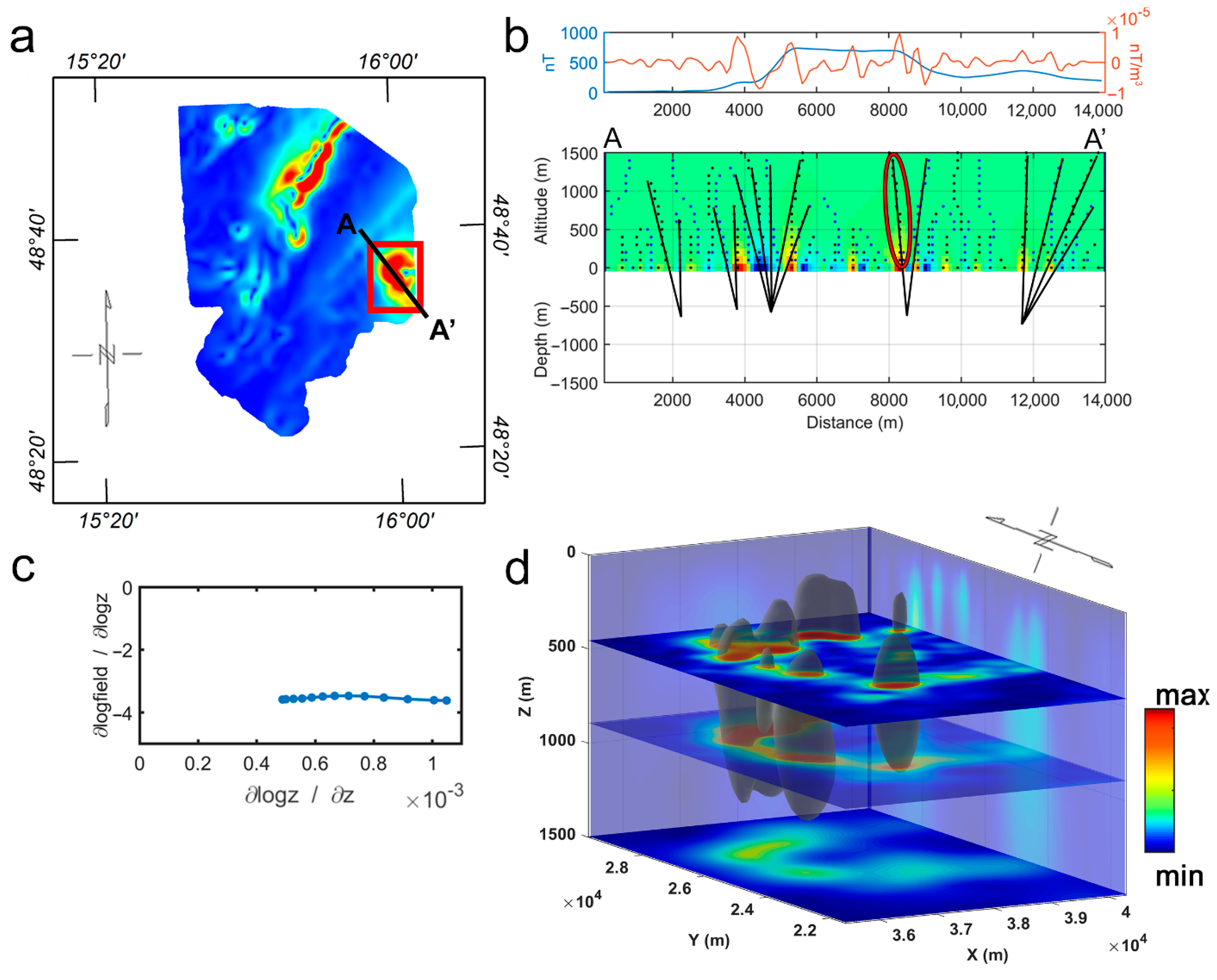
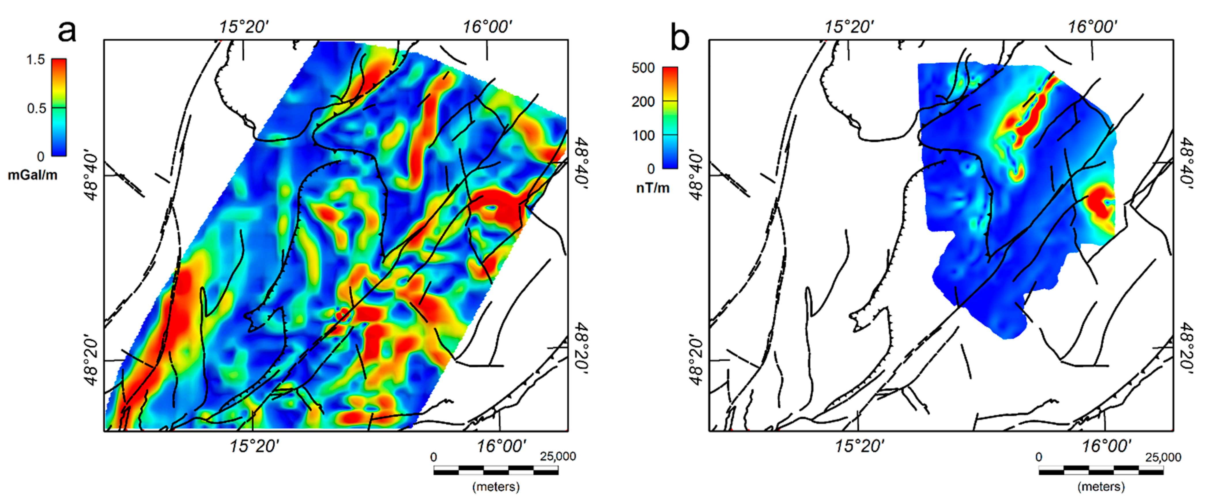
4.1. EHD

The EHD technique was applied to the gravimetric and aeromagnetic data of the survey area by varying the terms of the summation ϕ (2) to visualize the horizontal limits of different scale sources placed at different depths based on a proper choice of weights wi, of the starting term of the summation and of the derivative order p.
Considering the gravity field as the first term of the summation (2) and adding derivatives of orders up to p = 6 we obtained an EHD medium-scale map clearly highlighting some NE-SW trends (Figure 7a). Some of these trends match with geological features in the Molasse Basin and in the south-east and north-east of the Moldanubian unity, whereas others suggest the existence of new structures not corresponding to known lineaments. As for the Diendorf main fault, there is no correspondence between the maximums of the medium-scale EHD and the entire length of the fault. Indeed, the fault pattern matches with the EHD maxima only on its central part, which is identical to the surface expression of the fault. For the Waitzendorf fault (WF) there is instead no correspondence with the maxima of the function.
As regards EHD on magnetic data we computed it by using the reduced field at the pole field as the first order of the summation (2) and taking into the summation orders of derivation up to p = 6 (Figure 7b). From this first medium-scale aeromagnetic EHD map it is possible to notice how the maxima of the function mainly fall on the edges of four sources. An elongated in the NE-SW direction in the north-central sector of the map, two small circular sources at the NW corner of the map and a circular at the eastern edge of the map.
Both the gravimetric and magnetic small-scale structured located by the EHD function will be further analyzed in terms of structural index and depth of the source imaging techniques.

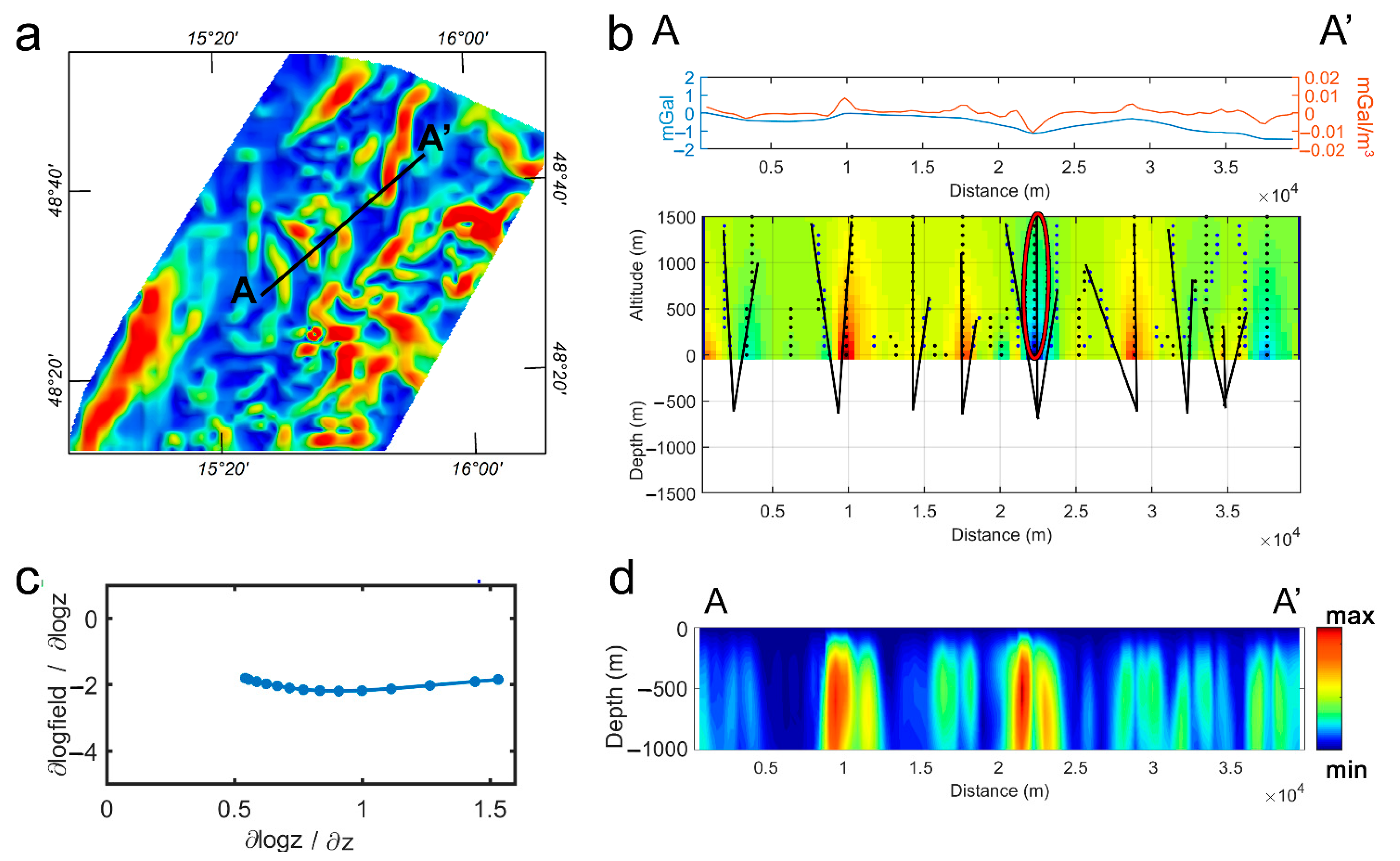
4.2. Multi-Ridge Geometric Method & DEXP

Based on the results of the small-scale EHD analysis, we picked up profiles and areas on which we carried out our DEXP analysis to determine the type of source and estimate its depth. For both the gravimetric and magnetic cases, the procedure included (e.g., [48]):
  • choice of the profile to be analyzed starting from the small-scale EHD map
  • for each chosen profile, selection of the order of derivatives and analysis of the ridges
  • selection of the ridges for the Multiridge Geometric Method [45] for detecting the average depth-to-the-sources
  • choice of the proper ridge for Euler Deconvolution for studying of the degree of homogeneity of the field (Multiridge Euler Deconvolution, e.g., [49])
  • from the degree of homogeneity obtained, we used the Scaling Function Method [50] to identify the structural index, taking into account the order p to be subtracted
  • calculation of the DEXP along a profile or on an area, using the structural index previously obtained. In the gravimetric cases the DEXP was calculated on the horizontal derivative of the field, while in the magnetic cases the DEXP was calculated on the total gradient of the field.
The chosen profiles cross perpendicularly several maxima displayed by the EHD gravimetric map, while the areas chosen for our analysis include circular maxima of the magnetic EHD map (Figure 8a and Figure 9a, respectively). Figure 8b and Figure 9b show our selection of ridges for applying the Multiridge Geometric Method and detecting the depth-to-the-sources. The plots report the ridges relative to the 3rd derivative of the gravity field computed along the two profiles AA’. Black dots are the maxima of the vertical gradient of the field, blue dots represent the maxima of the horizontal gradient of the field, black solid lines join the ridges and extrapolate them from the measurement plane to the source position [45], the red ellipse shows the ridge chosen for the evaluation of the homogeneity degree by Euler Deconvolution analysis. Figure 8b,c and Figure 9b,c show our analysis on structural index applying the Scaling Function Method. The Scaling Function Method is a multiscale method based on the study of the scaling function of potential fields that allows the retrieval of source parameters such as depth and structural index through an analysis along ridges. Following the method, the intercept with the y-axis of the scaling function τm vs. the reciprocal of the altitude 1/z, yields an estimate of the homogeneity degree n and, in turn, of the structural index N. We recall that homogeneous functions of degree n being the potential fields of simple sources, the degree of homogeneity can be expressed as: n = −N + p, where p is the derivative order of the potential field and N is the structural index, whose value varies from 0 to 3 for the magnetic case and from −1 to 2 for the gravity case, based on the homogeneous source type (e.g., [6,51]).
The Scaling Function analysis yielded values of N around −1 for gravity data and 1 for magnetic data. Those values refer to contact-like and to dyke-like structures, for the gravity and magnetic data, respectively [51]. Figure 8d and Figure 6d show the 2D and 3D imaging of the sources along the chosen profile and the chosen area of analysis, respectively. The depth to the sources, highlighted by the maxima of the DEXP signal, is larger than 500 m for the contact-like structures depicted by gravity data (Figure 8d) and about 450 m for the dyke-like structures depicted by magnetic data (Figure 9d); an average acquisition height of 100 m should be subtracted from the DEXP outcome for magnetic data. Based on the inferred values of structural indices, the found depths refer to the top of the structures.

5. Discussion and Conclusions

The purpose of this study was the characterization of sub-surface structures from geophysical data over a section of the Diendorf Fault System, on the south-eastern edge of the Bohemian Massif, Austria. The study area is part of a geologically complex area located in an area where the Bohemian Massif is in close vicinity to the Alpine-Carpathian thrust front. The land gravimetric and high-resolution airborne (magnetic, electromagnetic and gamma-ray) data acquired by the GBA were processed through advanced techniques and recent methods of analysis of potential field data. Our results confirmed the existence of some geological structures already known in the survey area (e.g., the MSZ and the central part of the DFS) and allowed the location of unknown structures with depths of a few hundred meters. Interestingly, the contact between the gneissic and igneous rocks (see Figure 1 and Figure 10) are often well captured by both methods. The Thaya window (Figure 1), bounded by the MSZ, DFS, and the WF, is separated into two units by the newly identified lineaments, both at shallow and larger depths. This is supported by new field observations proposing to subdivide the Thaya window into two nappes [20]. In general, most lineaments identified in the crystalline rocks west of the DFS may be connected either to mapped contacts between different geological units or to geological faults (Figure 10). However, it must be verified in the field if these can be associated with not yet mapped faults, or if they may be an expression of the highly deformed and folded rocks within the area. East of the DFS, the correlation between mapped geological features and lineaments is more challenging, as the Neogene sediments of the Molasse Basin cover the surface (see dark green areas in Figure 1 and Figure 10). The deeper structures are not exposed and therefore not well-known.
The use of the EHD method on potential field data enables us to infer the existence of different structural features whose horizontal limits are clearly visible from the medium-scale gravimetric and magnetic EHD maps. Some of the gravity EHD-lineaments match with known structures, whereas others suggest unknown structures (Figure 10). Specifically, we found that in the western region, almost all the EHD gravity maxima are well-correlated with already known geological structures; in the eastern/central sectors of the map, instead, half of the EHD gravity maxima identify previously unknown structures (Figure 7a).
Furthermore, the features shown by the magnetic data EHD correlate with areas of strong resistivity contrasts and with gamma-ray anomalies (Figure 6). In contrast, the gamma-ray anomalies highlight the strike of the WF, whereas deeper sources of the gravity and magnetic data do not show pronounced lineaments. This suggests that the WF is either not a deep-reaching feature or that the offset along the fault is not large enough to create material differences in the deeper levels.
The use of the DEXP method, applied to areas of the survey area that were found to be interesting based on the EHD analysis made it possible to:
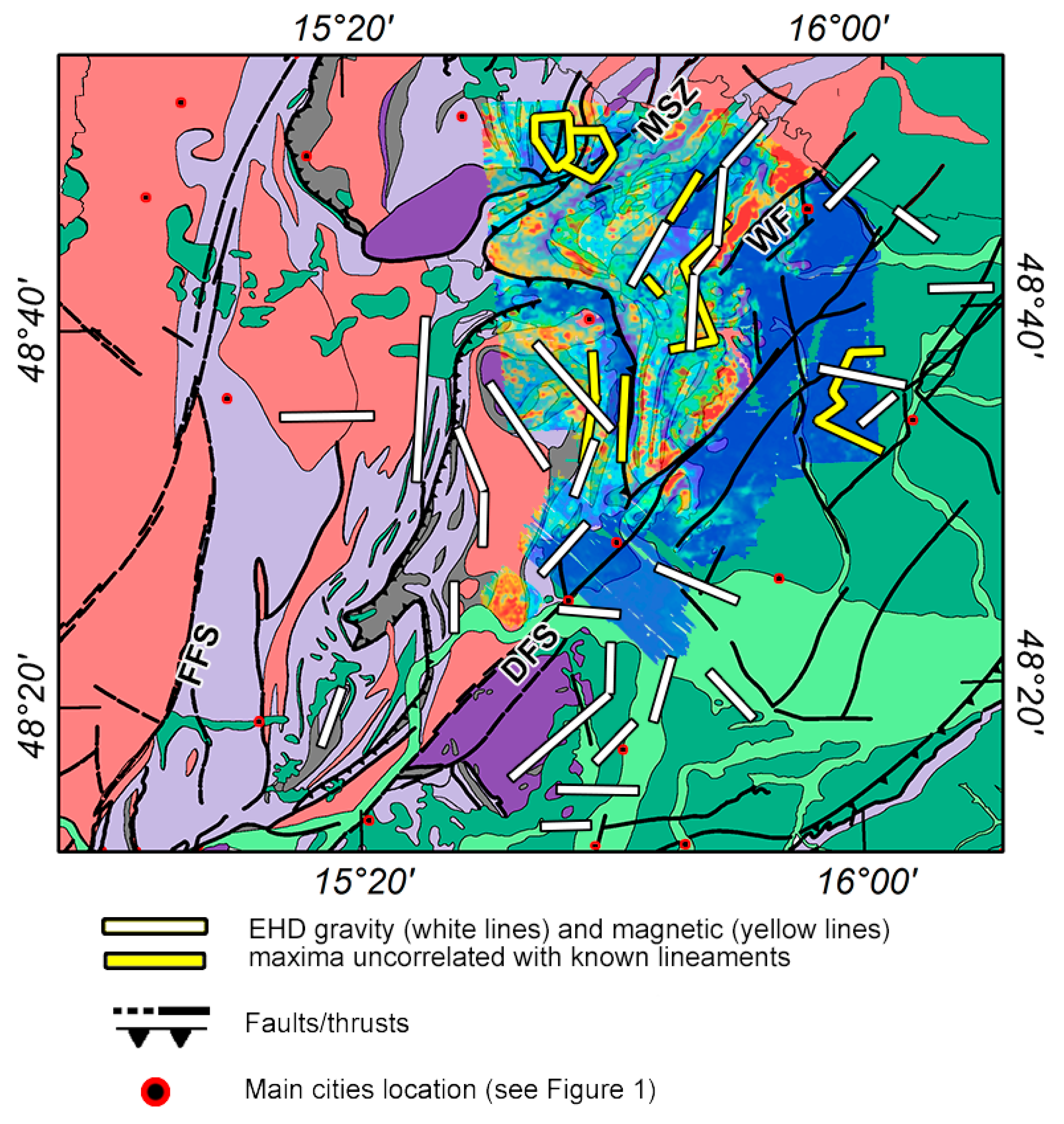
  • Locate a series of sub-surface contacts within the Moldanubian unit and in the Molasse Basin from 2D imaging on gravimetric data, highlighted as DEXP maxima. Given the good correspondence between many already known faults (e.g., part of the Diendorf fault and some faults affecting the Molasse Basin) and the maxima of the medium-scale EHD function and based on the structural indices value (equal to –1), we assume that the maximums identified by the DEXP analysis represent the top of previously unknown subsurface faults. The depth-to-the-top depth of the top of these faults is larger than 500 m.
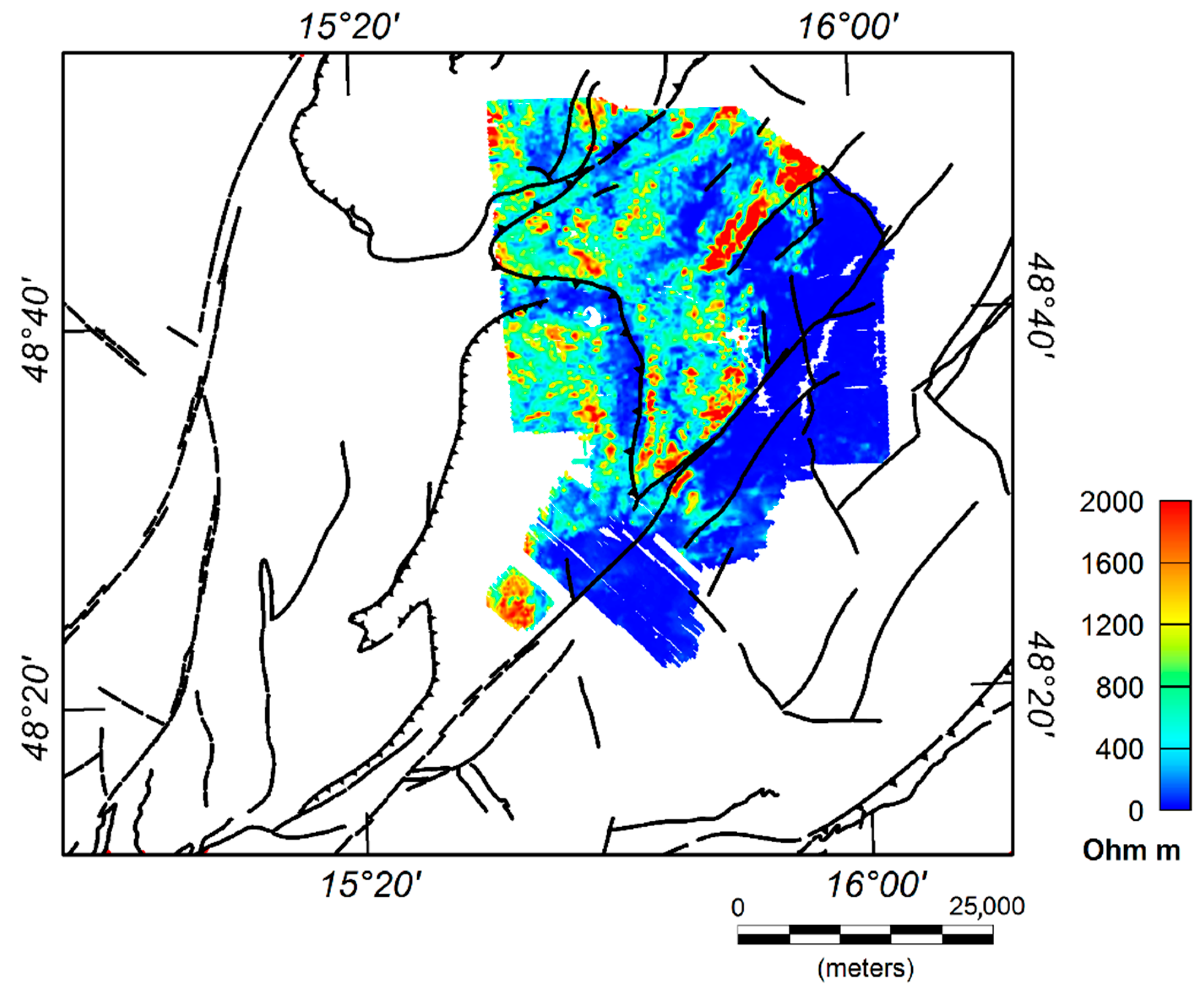
  • Highlighted from 3D imaging on magnetic data is a series of surface magnetized structures (about 450 m deep) that could represent magmatic intrusions. In fact, the central section of the magnetic dataset falls within an area geologically known as Thaya Window—a tectonic window that emerges between the Moldanubian tassels [19]. Furthermore, a part of the magnetized area inside it also presents a strong contrast of resistivity, as can be seen from the inversion model relating to the aero-electromagnetic data.
  • We add that several structures identified thanks to the magnetic data imaging do not have correspondence on the geological map, nor on the resistivity data map. This could be related to the large depth of the structures identified by the analysis of aeromagnetic data (of the order of hundreds of meters) that are masked by covering sediments. In fact, the depth of investigation of the AEM method in the Pulkau area is at most 150 m, not large enough to be able to locate possible resistive bodies and structures below the covering materials. Finally, the widespread presence of magmatic intrusions of the Cadomian age in the area [10], would suggest that the magnetized sources found in this work can be interpreted as intrusions.
We remark that, each geophysical methodology being sensitive to specific physical parameters, the correlation among the results from different methods and between geology and the different geophysical outcomes is strongly dependent on lithological features of the surveyed area.
In conclusion, we highlighted the excellent resolving power of edge-analysis and imaging techniques in a complex geological area namely the Diendorf Fault System area. We located several lineaments both on maps and at depth, which could be the subject of further studies in greater detail. More closely spaced land and airborne data acquired within future research projects would surely improve the accuracy in detection of local-scale geological features. In addition, the information on some of the parameters of the sources provided by the imaging of these areas could be used as geological constraints for inversion models.

Author Contributions

Conceptualization, V.P., E.H. and I.S.; methodology, V.P., I.S., M.M. and G.P.D.; validation, V.P., E.H., I.S., M.M. and R.S.; Writing—original draft preparation, V.P., E.H., I.S. and G.P.D.; Writing—review and editing, V.P., E.H., I.S. and G.P.D.; Figures Editing, M.M. All authors discussed the data, their processing, and the models. All authors have read and agreed to the published version of the manuscript.

Funding

Project 2022 GeoERA (HIKE): this project received funding from the European Union’s Horizon 2020 research and innovation programme under grant agreement No. 731166. Teaching award funds of the University of Cagliari: Project ID 44758 (Dipartimento di Ingegneria Civile, Ambientale e Architettura)–Gian Piero Deidda.

Data Availability Statement

The gravity dataset used in this study are openly available in GFZ Data Services at https://dataservices.gfz-potsdam.de/panmetaworks/showshort.php?id=8039528e-3ada-11eb-9603-497c92695674 (accessed on 3 March 2022). The magnetic, FDEM and gamma-ray data analyzed in this study are available on request from the corresponding author and will be soon openly available on the Tethys Research Data Repository [https://tethys.at/].

Acknowledgments

We would like to thank the aerogeophysics team led by Klaus Motschka and Wolfgang Seiberl for executing the surveys and providing the data. We acknowledge Emilia Miranda for early processing on gravity and magnetic data. We are grateful to two anonymous reviewers for their constructive and helpful comments.

Conflicts of Interest

The authors declare no conflict of interest.

References

  1. Blakely, R.J. Potential Theory in Gravity and Magnetic Applications; Cambridge University Press: Cambridge, UK, 1996. [Google Scholar] [CrossRef]
  2. Eppelbaum, L.V. Geophysical Potential Fields: Geological and Environmental Applications; Elsevier: Amsterdam, The Netherlands, 2019. [Google Scholar]
  3. IAEA-TECDOC-1363. Guidelines for Radioelement Mapping Using Gamma Ray Spectrometry Data. International Atomic Energy Agency (IAEA). 2003. Available online: https://www-pub.iaea.org/mtcd/publications/pdf/te_1363_web.pdf (accessed on 3 March 2022).
  4. Zuzana, S.; Vladislav, R.; Bedřich, M. Effect of small potassium-rich dykes on regional gamma-spectrometry image of a potassium-poor volcanic complex: A case from the Doupovské hory Volcanic Complex, NW Czech Republic. J. Volcanol. Geotherm. Res. 2009, 187, 26–32. [Google Scholar] [CrossRef]
  5. Paoletti, V.; Gruber, S.; Varley, N.; D’Antonio, M.; Supper, R.; Motschka, K. Insights into the Structure and Surface Geology of Isla Socorro, Mexico, from Airborne Magnetic and Gamma-Ray Surveys. Surv. Geophys. 2016, 37, 601–623. [Google Scholar] [CrossRef]
  6. Milano, M.; Fedi, M.; Fairhead, J.D. The deep crust beneath the Trans-European Suture Zone from a multiscale magnetic model. J. Geophys. Res. Solid Earth 2016, 121, 6276–6292. [Google Scholar] [CrossRef] [Green Version]
  7. Milano, M.; Fedi, M.; Fairhead, J.D. Joint analysis of the magnetic field and total gradient intensity in central Europe. Solid Earth 2019, 10, 697–712. [Google Scholar] [CrossRef] [Green Version]
  8. Paoletti, V.; Milano, M.; Baniamerian, J.; Fedi, M. Magnetic Field Imaging of Salt Structures at Nordkapp Basin, Barents Sea. Geophys. Res. Lett. 2020, 47, e2020GL089026. [Google Scholar] [CrossRef]
  9. Roštínský, P.; Pospíšil, L.; Švábenský, O. Recent geodynamic and geomorphological analyses of the Diendorf–Čebín Tectonic Zone, Czech Republic. Tectonophysics 2013, 599, 45–66. [Google Scholar] [CrossRef]
  10. Pospíšil, L.; Roštínský, P.; Švábenský, O.; Weigel, J.; Witiska, M. Active tectonics in the eastern margin of the Bohemian massif-based on the geophysical, geomorphological and GPS data. Acta Geodyn. Geomater. 2012, 9, 315–329. [Google Scholar]
  11. Decker, K. Tectonic Assessment of integrated Geological, geophysical, Morphological and structural Geological Data. Project N-C-036/F/98 Ground Potential of the Horn–Hollabrunn Environmental Area; Geologische Bundesanstalt: Wien, Austria, 1999. (In German) [Google Scholar]
  12. Schermann, O. Über Horizontalseitenverschiebungen arn Ostrand der Böhmischen Masse. Mitt. Ges. Geol. Bergbaustud. 1965, 16, 89–103. (In German) [Google Scholar]
  13. Figdor, H.; Scheidegger, A.E. Geophysical investigation of the Diendorf Fault. Verh. Der Geol. Bundesanst. 1977, 3, 243–270. (In German) [Google Scholar]
  14. Griesmeier, G.E.U.; Iglseder, C.; Schuster, R.; Petrakakis, K. Polyphase deformation along the South Bohemian Batholith-Moldanubian nappes boundary—The Freyenstein Fault System (Bohemian Massif/Austria). Austrian J. Earth Sci. 2020, 113, 139–153. [Google Scholar] [CrossRef]
  15. Seiberl, W.; Heinz, H. Aerogeophysikalische Vermessung Im Bereich Der Kremser Bucht. Technical Report. Vienna: Geological Survey of Austria, May 1986. Available online: http://opac.geologie.ac.at/ais312/dokumente/AeroGeoPh_1986_KremserBucht.pdf (accessed on 3 March 2022). (In German).
  16. Seiberl, W.; Heinz, H. Aerogeophysikalische Vermessung Im Raum Ziersdorf. Technical Report. Vienna: Geological Survey of Austria, October 1986. Available online: http://opac.geologie.ac.at/ais312/dokumente/AeroGeoPh_1986_Ziersdorf.pdf (accessed on 3 March 2022). (In German).
  17. Seiberl, W.; Roetzel, R. Aerogeophysikalische Vermessung Im Bereich Geras, Niederösterreich. Technical Report. Vienna: Geological Survey of Austria, August 1998. Available online: http://opac.geologie.ac.at/ais312/dokumente/AeroGeoPh_1998_Geras.pdf (accessed on 3 March 2022). (In German).
  18. Seiberl, W.; Roetzel, R.; Pirkl, H.R. Aerogeophysikalische Vermessung im Bereich von Pulkau/NÖ.’ Technical report. Vienna: Geological Survey of Austria, May 1996. Available online: http://opac.geologie.ac.at/ais312/dokumente/AeroGeoPh_1996_Pulkau.pdf (accessed on 3 March 2022). (In German).
  19. Štípská, P.; Schulmann, K.; Höck, V. Complex metamorphic zonation of the Thaya dome: Result of buckling and gravitational collapse of an imbricated nappe sequence. Geol. Soc. London, Spéc. Publ. 1999, 169, 197–211. [Google Scholar] [CrossRef]
  20. Linner, M.; Roetzel, R.; Huet, B.; Hintersberger, E. A new subdivision for the Moravian Superunit—The redefined Pleißing and the newly defined Pulkau nappe. In Proceedings of the 4th Friends of the Bohemian Massif Meeting, Freistadt, Austria, 10 July–10 October 2021. [Google Scholar]
  21. Farr, T.G.; Rosen, P.A.; Caro, E.; Crippen, R.; Duren, R.; Hensley, S.; Kobrick, M.; Paller, M.; Rodriguez, E.; Roth, L.; et al. The Shuttle Radar Topography Mission. Rev. Geophys. 2007, 45, RG2004. [Google Scholar] [CrossRef] [Green Version]
  22. Schuster, R.; Daurer, A.; Krenmayr, H.G.; Linner, M.; Mandl, G.W.; Pestal, G.; Reitner, J. Rocky Austria: The Geology of Austria-Brief and Colourful 2014. Geological Survey of Austria. Available online: https://geolba.maps.arcgis.com/apps/webappviewer/index.html?id=0e19d373a13d4eb19da3544ce15f35ec (accessed on 3 March 2022).
  23. Zych, D. Messungen Der Erdmagnetischen Vertikalintensität Und Suszeptibilitätsuntersuchungen Durch Die Ömv-Ag Als Beitrag Zur Kohlenwasserstoffexploration in Österreich; Zentralanstalt für Meteorologie und Geodynamik (ZAMG) Publikation: Vienna, Austria, 1985. (In German) [Google Scholar]
  24. Hösch, K.; Steinhauser, P. Gesteinsphysikalische Untersuchungen in Der Östlichen Böhmischen Masse Niederösterreichs; Bericht Bund/Bundesländer-Rohstoffprojekt N-C-006b/81, Bibl. Geol. B.-A./Wiss. Archiv Nr. A 06299–R, 28 S., 7 Abb.: Wien, Austria, 1985. (In German) [Google Scholar]
  25. Scheidegger, A.E. Untersuchungen des Beanspruchungsplanes im Einflußgebiet der Diendorfer Störung; Jahrbuch Der Geologischen Bundesanstalt: Vienna, Austria, 1976; Volume 119, pp. 83–95. (In German) [Google Scholar]
  26. Hammerl, C.; Lenhardt, W. Erdbeben in Niederösterreich von 1000 bis 2009 n. Chr. Abh. Der Geol. Bundesanst. 2013, 67, 297. (In German) [Google Scholar]
  27. Pospíšil, L.; Švábenský, O.; Weigel, J.; Witiska, M. Geological constraints on the GPS and precise levelling measurements along the DIENDORF-ČEBÍN tectonic zone. Acta Geodyn. Geomater. 2010, 7, 317–333. [Google Scholar]
  28. Vyskočil, P. Recent crustal movements in the Bohemian Massif. Tectonophysics 1975, 29, 349–358. [Google Scholar] [CrossRef]
  29. Vyskočil, P. Recent crustal movements their properties and results of studies at the territory of Czech Republic. In Seismicity, Neotectonics, and Recent Dynamics with Special Regard to the Territory of Czech Republic; Research Institute of Geodesy, Topography and Cartography: Zdiby, Czech Republic, 1996; pp. 77–120. ISBN 80-85881-04-7. [Google Scholar]
  30. Leichmann, J.; Hejl, E. Quaternary tectonics at the eastern border of the Bohemian Massif: New outcrop evidence. Geol. Mag. 1996, 133, 103–105. [Google Scholar] [CrossRef]
  31. Meurers, B.; Ruess, D. A new Bouguer gravity map of Austria. Austrian J. Earth Sci. 2009, 102, 62–70. [Google Scholar]
  32. Ruess, D. Der Beitrag Österreichs an UNIGRACE—Unification of Gravity Systems of Central and Eastern European Countries. VGI—Osterr. Z. Für Vermess. Und Geoinf. 2002, 90, 129–139. Available online: https://de.readkong.com/page/der-beitrag-osterreichs-an-unigrace-uni-cation-of-gravity-7039576 (accessed on 3 March 2022).
  33. Meurers, B.; Ruess, D.; Graf, J. A program system for high precise Bouguer gravity gravity determination. In Proceedings of the 8th International Meeting on Alpine Gravimetry: Leoben 2000; Österreichische Beiträge zu Meteorologie und Geophysik; ZAMG: Wien, Austria, 2001; pp. 217–226. [Google Scholar]
  34. Aric, K.; Gutdeutsch, R.; Heinz, H.; Meurers, B.; Seiberl, W.; Adam, A.; Smythe, D. Geophysical Investigations in the Southern Bohemian Massif. Jahrbuch Der Geologischen Bundesanstalt 1997, 140, 9–28. [Google Scholar]
  35. Meurers, B.; Ruess, D. Compilation of a new Bouguer gravity data base in Austria. VGI—Osterr. Z. Für. Vermess. Und. Geoinf. 2007, 2, 90–94. [Google Scholar]
  36. Motschka, K. Aerogeophysics in Austria. Bull. Geol. Surv. Jpn. 2001, 52, 83–88. [Google Scholar]
  37. Paoletti, V.; D’Antonio, M.; Rapolla, A. The structural setting of the Ischia Island (Phlegrean Volcanic District, Southern Italy): Inferences from geophysics and geochemistry. J. Volcanol. Geotherm. Res. 2013, 249, 155–173. [Google Scholar] [CrossRef]
  38. Supper, R.; Baroň, I.; Ottowitz, D.; Motschka, K.; Gruber, S.; Winkler, E.; Jochum, B.; Römer, A. Airborne geophysical mapping as an innovative methodology for landslide investigation: Evaluation of results from the Gschliefgraben landslide, Austria. Nat. Hazards Earth Syst. Sci. 2013, 13, 3313–3328. [Google Scholar] [CrossRef] [Green Version]
  39. Bohrson, W.A.; Reid, M.R. Petrogenesis of alkaline basalts from Socorro Island, Mexico: Trace element evidence for contamination of ocean island basalt in the shallow ocean crust. J. Geophys. Res. Earth Surf. 1995, 100, 24555–24576. [Google Scholar] [CrossRef]
  40. Grasty, R.; Minty, B.R.S. A Guide to the Technical Specifications for Airborne Gamma-Ray Surveys; Australian Geological Survey Organization: Canberra, Australia, 1995; ISBN 0642223661. [Google Scholar]
  41. Fedi, M. Multiscale derivative analysis: A new tool to enhance detection of gravity source boundaries at various scales. Geophys. Res. Lett. 2002, 29, 507. [Google Scholar] [CrossRef]
  42. Fedi, M.; Florio, G. Detection of potential fields source boundaries by enhanced horizontal derivative method. Geophys. Prospect. 2001, 49, 40–58. [Google Scholar] [CrossRef]
  43. Luiso, P.; Paoletti, V.; Nappi, R.; La Manna, M.; Cella, F.; Gaudiosi, G.; Fedi, M.; Iorio, M. A multidisciplinary approach to characterize the geometry of active faults: The example of Mt. Massico, Southern Italy. Geophys. J. Int. 2018, 213, 1673–1681. [Google Scholar] [CrossRef]
  44. Luiso, P.; Paoletti, V.; Nappi, R.; Gaudiosi, G.; Cella, F.; Fedi, M. Testing the value of a multi-scale gravimetric analysis in characterizing active fault 2 geometry at hypocentral depths: The 2016-2017 Central Italy seismic sequence. Ann. Geophys. 2018, 61, 29. [Google Scholar] [CrossRef]
  45. Fedi, M.; Florio, G.; Quarta, T.A. Multiridge analysis of potential fields: Geometric method and reduced Euler deconvolution. Geophysics 2009, 74, L53–L65. [Google Scholar] [CrossRef]
  46. Fedi, M. DEXP: A fast method to determine the depth and the structural index of potential fields sources. Geophysics 2007, 72, I1–I11. [Google Scholar] [CrossRef]
  47. Fedi, M.; Pilkington, M. Understanding imaging methods for potential field data. Geophysics 2012, 77, G13–G24. [Google Scholar] [CrossRef] [Green Version]
  48. Paoletti, V.; Buggi, A.; Pašteka, R. UXO Detection by Multiscale Potential Field Methods. Pure Appl. Geophys. 2019, 176, 4363–4381. [Google Scholar] [CrossRef]
  49. Paoletti, V.; Ialongo, S.; Florio, G.; Fedi, M.; Cella, F. Self-constrained inversion of potential fields. Geophys. J. Int. 2013, 195, 854–869. [Google Scholar] [CrossRef] [Green Version]
  50. Florio, G.; Fedi, M.; Rapolla, A. Interpretation of regional aeromagnetic data by the scaling function method: The case of Southern Apennines (Italy). Geophys. Prospect. 2009, 57, 479–489. [Google Scholar] [CrossRef]
  51. Cella, F.; Fedi, M. Inversion of potential field data using the structural index as weighting function rate decay. Geophys. Prospect. 2011, 60, 313–336. [Google Scholar] [CrossRef]
Figure 2. Survey layouts. (a) Acquisition points of gravimetric data (unevenly distributed in black) and acquisition lines of airborne data (in red); measurement areas: 1: Geras, 2: Pulkau north, 3: Pulkau, 4: Kamptal-Ziersdorf 5: Kremser Bucht; (b) clearance of the airborne data.
Remotesensing 14 01807 g002
Figure 3. Bouguer map of the study area. The main maxima, with amplitude of about 30 mGal, are located in the central and eastern sections of the map and are often edged by the known faults of the area.
Remotesensing 14 01807 g003
Figure 4. RTP Aeromagnetic map of the study area. Two main anomalies, with amplitude of about 500 nT, are located in the northern and eastern sides of the map.
Remotesensing 14 01807 g004
Figure 5. Aero-electromagnetic resistivity map of the study area. The main maxima, with amplitude of about 1500–2000 Ohm m, are correlated with the known faults and are located in the central and western sectors of the survey area. The region of minima (dark blue) coincides with the extent of the Neogene Molasse Basin and the location of smaller sedimentary basins within the Bohemian Massif.
Remotesensing 14 01807 g005
Figure 6. (a) Aero-radiometric potassium data (K); (b) Aero-radiometric thorium data (Th); (c) Aero-radiometric uranium data (U). The main maxima in the three maps are well-correlated with the known faults and geological units of the survey area.
Remotesensing 14 01807 g006
Figure 7. EHD map of the survey area: (a) Medium-scale EHD map of gravity data obtained using derivatives of order up to p = 6; (b) medium-scale EHD map of aeromagnetic data obtained using derivatives of order up to p = 6.
Remotesensing 14 01807 g007
Figure 8. Structural index and depth estimation for gravimetric data: (a) EHD map highlighting lineaments with overlaid the profile chosen for our analysis; (b) ridges relative to the 3rd derivative of the gravity field computed along the profile AA’; (c) evaluation of the SI N by the scaling function analysis; (d) 2D imaging of the sources of the area on horizontal gradient of gravity data along the chosen profile; the depth to the sources is shown by the maxima of the DEXP signal (normalized dimensionless units are used).
Remotesensing 14 01807 g008
Figure 9. Structural index and depth estimation for magnetic data: (a) EHD map showing the circular pattern chosen for our analysis (red rectangle); (b) ridges relative to the 3rd derivative of the magnetic field computed along the profile AA’; (c) evaluation of the SI N by the scaling function analysis; (d) 3D imaging of the sources in the analysis area performed on total gradient of magnetic data; the depth to the sources is shown by the maxima of the DEXP signal (normalized dimensionless units are used). An average acquisition height of 100 m should be subtracted from the outcomes of the Multiridge Geometric Method and DEXP.
Remotesensing 14 01807 g009
Figure 10. Correlation between geology (refer to Figure 1), resistivity values deriving from the EM measurements (colored contouring) and the main maxima of the medium-scale EHD function on gravity (white lines) and magnetic (yellow lines) data. West of the DFS, the identified lineaments correlate generally well with faults, thrusts, or contacts between mapped geological units. Eastward, in the Molasse Basin, the correlation is not as obvious, but the Neogene sedimentary infill of the Molasse Basin covers deeper seated structures; therefore, these could be newly discovered faults or geological contacts.
Remotesensing 14 01807 g010
Table 1. Vintage data sets measured using different technical equipment and survey specification.
Aerogeophysical Survey/yMagnetic DeviceElectromagnetic Device/FrequenciesRadiometric DeviceData per sec (Mag/EM/Rad)Average Line Spacing [m]
Kremser Bucht/1983G-801/3DIGHEM II/900 Hz (vert./coaxial), 3600 Hz (horiz./coplanar)GR-800 B1/4/1200
Kamptal-Ziersdorf/1983G-801/3DIGHEM II/900 Hz (vert./coaxial), 3600 Hz (horiz./coplanar)GR-800 B1/4/1200
Pulkau/1994Scintrex CS-2DIGHEM II/900 Hz (vert./coaxial), 7200 Hz (horiz./coplanar)Scintrex PGAM-10005/10/1250
Pulkau north/1995Scintrex CS-2DIGHEM II/900 Hz (vert./coaxial), 7200 Hz (horiz./coplanar)Scintrex PGAM-10005/10/1200
Geras/1996–1997Scintrex CS-2GEOTECH “Hummingbird”/434 Hz (vertic./coplanar), 3212 Hz (horiz./coaxial), 7002 Hz(vertic./coplanar), 34,133 Hz (horiz./coaxial)Scintrex PGAM-10005/10/1200
Publisher’s Note: MDPI stays neutral with regard to jurisdictional claims in published maps and institutional affiliations.

