Article

Constructing a Large-Scale Urban Land Subsidence Prediction Method Based on Neural Network Algorithm from the Perspective of Multiple Factors

1
Faculty of Land Resources Engineering, Kunming University of Science and Technology, Kunming 650093, China
2
School of Earth Sciences, Yunnan University, Kunming 650500, China
3
Engineering Research Center of Domestic High-Resolution Satellite Remote Sensing Geology for Universities of Yunnan Province, Kunming 650500, China
4
MNR Key Laboratory of Sanjiang Metallogeny and Resources Exploration & Utilization, Kunming 650051, China
*
Author to whom correspondence should be addressed.
These authors contributed equally to this work.
Remote Sens. 2022, 14(8), 1803; https://doi.org/10.3390/rs14081803
Submission received: 17 February 2022 / Revised: 27 March 2022 / Accepted: 6 April 2022 / Published: 8 April 2022
(This article belongs to the Section Engineering Remote Sensing)

Abstract

:
The existing neural network model in urban land-subsidence prediction is over-reliant on historical subsidence data. It cannot accurately capture or predict the fluctuation in the sequence deformation, while the improper selection of training samples directly affects its final prediction accuracy for large-scale urban land subsidence. In response to the shortcomings of previous urban land-subsidence predictions, a subsidence prediction method based on a neural network algorithm was constructed in this study, from a multi-factorial perspective. Furthermore, the scientific selection of a large range of training samples was controlled using a K-shape clustering algorithm in order to produce this high-precision urban land subsidence prediction method. Specifically, the main urban area of Kunming city was taken as the research object, LiCSBAS technology was adopted to obtain the information on the land-subsidence deformation in the main urban area of Kunming city from 2018–2021, and the relationship between the land subsidence and its influencing factors was revealed through a grey correlation analysis. Hydrogeology, geological structure, fault, groundwater, high-speed railways, and high-rise buildings were selected as the influencing factors. Reliable subsidence training samples were obtained by using the time-series clustering K-shape algorithm. Particle swarm optimization–back propagation (PSO-BP) was constructed from a multi-factorial perspective. Additionally, after the neural network algorithm was employed to predict the urban land subsidence, the fluctuation in the urban land-subsidence sequence deformation was predicted with the LSTM neural network from a multi-factorial perspective. Finally, the large-scale urban land-subsidence prediction was performed. The results demonstrate that the maximum subsidence rate in the main urban area of Kunming reached −30.591 mm a 1 between 2018 and 2021. Moreover, there were four main significant subsidence areas in the whole region, with uneven distribution characteristics along Dianchi: within the range of 200–600 m from large commercial areas and high-rise buildings, within the range of 400–1200 m from the under-construction subway, and within the annual average. The land subsidence tended to occur within the range of 109–117 mm of annual average rainfall. Furthermore, the development of faults destroys the stability of the soil structure and further aggravates the land subsidence. Hydrogeology, geological structure, and groundwater also influence the land subsidence in the main urban area of Kunming. The reliability of the training sample selection can be improved by clustering the subsidence data with the K-shape algorithm, and the constructed multi-factorial PSO-BP method can effectively predict the subsidence rate with a mean squared error (MSE) of 4.820 mm. The prediction accuracy was slightly improved compared to the non-clustered prediction. We used the constructed multi-factorial long short-term memory (LSTM) model to predict the next ten periods of any time-series subsidence data in the three types of cluster data (Cluster 1, Cluster 2, and Cluster 3). The root mean square errors (RMSE) were 0.445, 1.475, and 1.468 mm; the absolute error ranges were 0.007–1.030, 0–3.001, and 0.401–3.679 mm; the errors (mean absolute error, MAE) were 0.319, 1.214, and 1.167 mm, respectively. Their prediction accuracy was significantly improved, and the predictions met the measurement specifications. Overall, the prediction method proposed from the multi-factorial perspective improves large-scale, high-accuracy urban land-subsidence prediction.

1. Introduction

Land subsidence is an environmental geological phenomenon in which regional ground elevation decreases with the compression of the surface soil of the earth’s crust under the action of natural and human factors [1]. It is one of the most common geological disasters worldwide [2]. In recent years, the degree and extent of land subsidence have been deepening and increasing along with the acceleration of urbanization in China. Meanwhile, urban areas are the entities most affected by land subsidence owing to various factors, such as the over-exploitation of groundwater, tunneling, and urban expansion, which are characterized by slow genesis, long duration, a wide impact range, complex causal mechanisms, and great difficulty in their prevention and control [2,3,4]. In the past 40 years, the losses caused by land subsidence in China have reached 300 billion. Urban land subsidence not only affects the productivity and lives of urban residents and traffic safety, but also severely hinders sustainable socioeconomic development [1]. Therefore, it is urgent and challenging to explore an effective method for predicting land subsidence [1].
Kunming, the capital and largest city of Yunnan Province in southwestern China, is located in the middle of the Yunnan–Guizhou Plateau, surrounded by the Dianchi Lake to the south and mountains on the remaining three sides. Located on China’s frontier with Southeast and South Asia, Kunming has implemented massive urban construction over the past two decades. During the process, a large amount of arable land and gardens has been occupied by high-rise buildings, roads, and other structures [5]. However, this large-scale urbanization has induced a series of geological hazards, such as landslides, subsidence, and ground cracks. In particular, the extent, amount, and rate of ground subsidence change from year to year, with an overall trend of increase, making it one of the most prominent geological hazards and significantly damaging houses, roads, canals, pipelines, and other forms of infrastructure [4]. Ground subsidence in Kunming is the loss of ground elevation caused by a combination of natural and human factors. The major natural factors include geological formations and hydrogeology, and the human factors primarily consist of groundwater mining and urban construction [6,7].
Interferometric synthetic aperture radar (InSAR) technology is an all-weather monitoring method, which has the advantages of large scale, low cost, high speed and high accuracy, and can be used for the precise measurement of surface deformation, such as in urban land subsidence [8,9,10], landslide monitoring [11,12], earthquake analysis [13], infrastructure assessment [14,15], and others [16]. With the development of high-resolution SAR (synthetic aperture radar), remote sensing technology has truly entered the era of high resolution, presenting high potential in the refined monitoring of surface deformation. Moreover, the data of the Earth observation satellite Sentinel-1A/B in the European Space Agency’s Copernicus program (Global Monitoring for Environment and Security, GMES) is free and open-access, providing users with rich and useful synthetic aperture radar data. However, the acquisition, storage, preprocessing, and a series of time-series parameter inversions of a large amount of image data in the monitoring area require excessive processing time, posing challenges to the computer performance, disk space, and other hardware conditions [17]. It is more challenging to monitor large-scale surface deformation. Concurrently, atmospheric delay error and phase unwrapping error are two of the main types of error in deformation inversion. Therefore, it is essential to handle atmospheric delay errors and phase-unwrapping errors when obtaining surface deformation information. An open-source InSAR time-series analysis method, LiCSBAS (the small-baseline subset within LiCSAR), proposed by Morishita et al. [17] for an automated Sentinel-1 InSAR processor, can effectively solve the problem that large-scale monitoring requires a significant amount of processing time and can overcome atmospheric delay errors and phase solution. Entanglement errors can be effectively controlled using LiCSBAS. Thus, it is especially suitable for the acquisition of large-scale urban land-subsidence deformation information.
Traditional land-subsidence prediction models are mainly divided into three categories: (1) physical process models, which use factors such as soil and water combined with geotechnics to model the physical process of land subsidence [18], based on the physical mechanism of subsidence, and perform predictions by simulating the subsidence process; (2) mathematical and statistical models, which usually adopt discrete time-series data to predict future subsidence states based on the mathematical and statistical prediction of historical subsidence [18]; and (3) neural network models, which generally employ the acquired subsidence data to predict future subsidence states through neural networks [19,20]. However, physical process models possess complex parameters, and the relevant data are difficult to obtain, significantly limiting their application [1]. The simple statistical laws of mathematical–-statistical models do not easily explain complex ground subsidence phenomena, and mathematical–statistical models frequently lack physical and geoscientific bases, while the accuracy of time-series methods is affected by the quality of historical data [1,21]. In recent years, neural network models have been widely applied in many fields [19,22,23]. Related studies revealed that the use of neural networks has achieved good results in the prediction of various types of engineering deformation. Meanwhile, urban land subsidence presents nonlinear characteristics, and neural networks have powerful nonlinear mapping capabilities, laying a theoretical foundation for the prediction of urban ground models using neural network models. However, the existing neural network models have the following three drawbacks: (i) they rely excessively on historical subsidence data, which only play a fitting role and cannot effectively make predictions; (ii) they cannot accurately capture or predict the fluctuations of sequence deformation and, therefore, cannot obtain satisfactory prediction results [21]; (iii) they are limited by the training samples, which only allow the prediction of small-scale subsidence and not large-scale subsidence. A literature review was performed to manage the drawbacks of existing neural network models for subsidence prediction and to perform large-scale urban land-subsidence predictions. It was demonstrated that researchers have established a land-subsidence prediction model based on machine learning from a multi-factorial perspective [24]. Under the determination of the nonlinear relationship between the influencing factors and land subsidence, an XGBoost (eXtreme Gradient Boosting) land-subsidence prediction model with good results (namely, the construction of a land-subsidence prediction model based on a neural network algorithm from a multi-factorial perspective) can provide a solution for the existing neural network model, which cannot perform land-subsidence prediction, and overcome the drawback of the model’s over-reliance on subsidence data. Regarding the drawback that existing neural network models cannot accurately capture or predict the fluctuation in the sequence deformation, InSAR deformation time-series prediction based on a long–short memory (LSTM) neural network has been proposed [21]. It can overcome the limitations of previous fitting analyses, which were based only on existing data, perform a multi-factorial prediction for a single subsidence point, and accurately capture and predict sequence deformation. Concerning large-scale urban ground subsidence, which has numerous types of subsidence sequence, the selection of training samples directly affects the final prediction accuracy. Since K-shape is a new time-series clustering algorithm [25] and can efficiently generate time-series clusters, it was chosen to cluster the subsidence time series.
The traditional artificial neural network (ANN) model, with its advantages of self-adaptation, self-learning, nonlinear mapping, and fault tolerance, especially BP (back propagation) neural network, has a high self-learning ability, which allows it to tackle complex deformation problems, while its output results are influenced by the initial weights and thresholds [21,26]. The genetic algorithm (GA) and the particle swarm optimization (PSO) algorithm are evolutionary computational techniques [27]. The genetic algorithm is based on Darwin’s theory of evolution [28]. The particle swarm optimization algorithm is inspired by the social behavior of flocks of birds and fish [28]. Both methods are employed for the global optimization of variables to obtain better prediction results. Therefore, genetic algorithms and particle swarm optimization algorithms can also be used to optimize the weights and biases of neural network models and, thus, improve the prediction accuracy of neural network models [29]. The K-shape time-series clustering algorithm proposed by John Paparrizos et al. [25] can efficiently compare sequences and compute sequence centers while ensuring scaling invariance, translation invariance, and transformation invariance. The main methods include shape-based distance (SBD) and computing the center of mass of the class (which preserves the shape and features of the class) based on the SBD. Long short-term memory neural networks are a special type of recurrent neural network (RNN), designed specifically for processing sequential data, and have unique advantages in learning time-series data features [21,30]. LSTM neural networks consist of two main components (the storage module and the gate module), which are responsible for stabilizing the transmission of information and the control over the information passed. Compared with traditional artificial neural networks, the storage and gate modules enable LSTM neural networks to better capture time-series data fluctuations and obtain desirable prediction results [31,32].
In summary, this study aims to address the drawbacks of the lack of reliable sample data for large-scale urban land-subsidence prediction and the existing neural network algorithms, which mostly fit, but rarely achieve prediction. Specifically, the main urban area of Kunming was taken as the research object. LiCSBAS technology was used to obtain the land-subsidence deformation information from 2018–2021 in the main urban area of Kunming. The time-series clustering K-shape algorithm was adopted to cluster the acquired land-subsidence time-series. Next, the clustered subsidence points were classified, and hydrogeology, geological structure, fault, groundwater, high-speed railways, and high-rise buildings were selected as the influencing factors. Subsequently, the PSO-BP neural network algorithm was constructed to predict the urban land subsidence from a multi-factorial perspective. Finally, the fluctuation in the urban land-subsidence sequence deformation was predicted using the LSTM neural network from a multi-factorial perspective in order to achieve large-scale, high-precision urban land-subsidence prediction.

2. Materials and Methods

2.1. Materials

2.1.1. Overview of the Study Area

The study area is located in Kunming, the capital of Yunnan Province, in southwestern China, as illustrated in Figure 1a. Kunming is currently one of the only large- and medium-sized cities experiencing ground subsidence in the western highlands of the continent in China, with a severe subsidence area of about 300 km2. Kunming is located in a fertile lake basin on the northern shore of Dianchi Lake, surrounded by mountains to the north, west, and east, with an altitude of 1900 m and a latitude just north of the Tropic of Cancer [4,7]. As of 2014, Kunming had a population of 6.6 million and an urban population of 4.5 million [33]. Due to its low latitude and high altitude, Kunming has one of the mildest climates in China, characterized by short, cool, dry winters, mild days and cool nights, and long, warm, humid summers [4].

2.1.2. Geological Background

The main urban area of Kunming is located in the Late Cenozoic fault basin, which is controlled by several Quaternary active fractures. As shown in Figure 1b, the study area has significant neotectonic movements, which are controlled especially by the north–south main active faults, which are mainly characterized by fault-block uplift and subsidence cutting by faults in different directions. Since the Late Cenozoic, the compressive stress in the north of the regional stress field has mainly been in the west, and the tensile stress is generated in the basin area bounded by the Puduhe fault (F54) and the Yiyun fault (F153). As a result, five sub-blocks, namely Xishan, Puji, Sheshan, Hei Longtan, and Baiyi, controlled by The Puji–Hangjia Village fault (F55), Heilongtan–Guandu fault (F150), and the Baiyi–Hengchuan fault (F149), are successively pulled northward (Figure 1b). Due to the control of the faults, the magnitude of the rift is different. Generally speaking, the magnitude of the sag is large in the south and relatively small in the north [34].
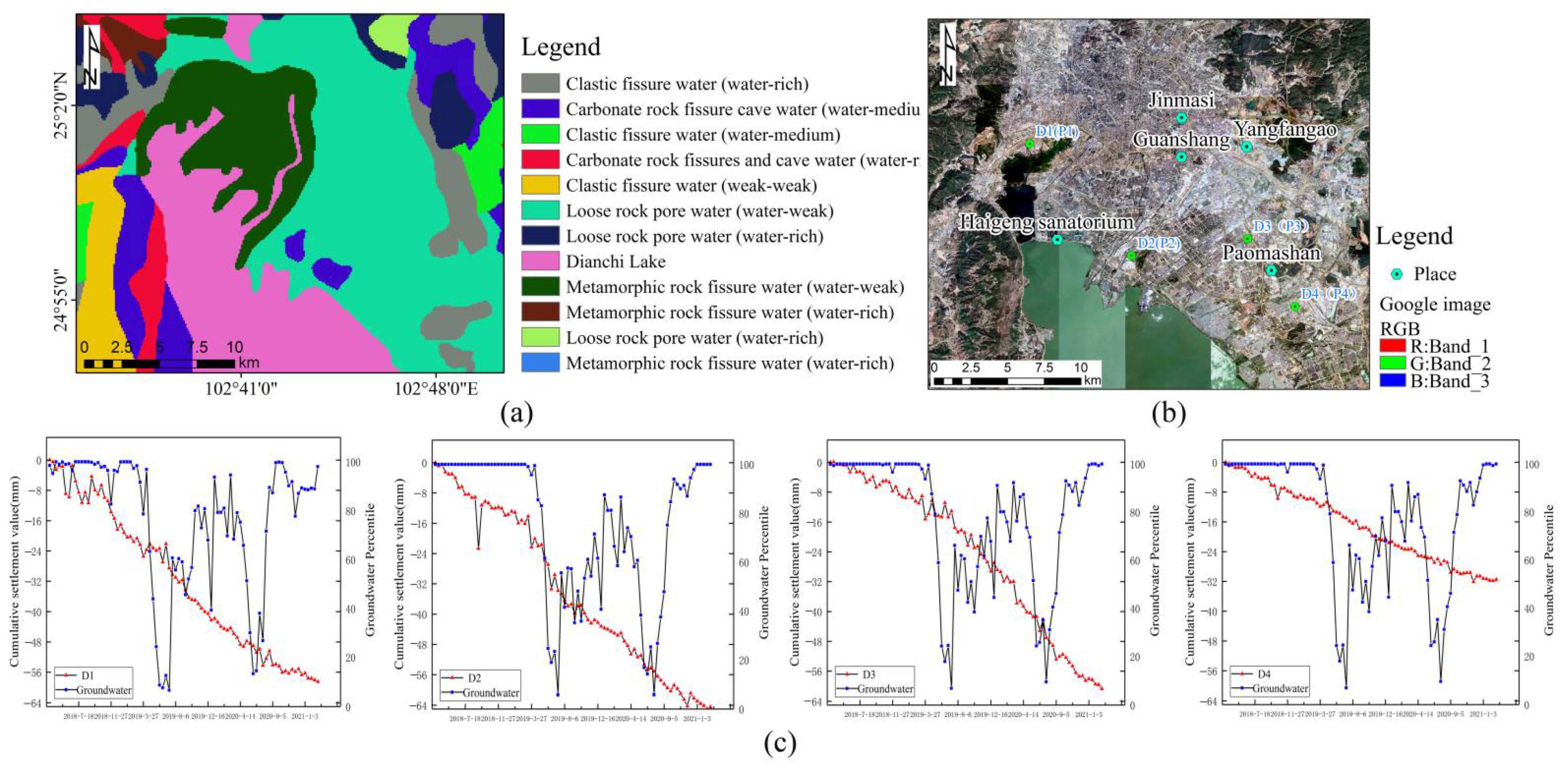
The main urban area of Kunming features widely developed Quaternary loose sedimentary layers and Quaternary accumulations of varying thicknesses distributed near the surface. The soils are composed of lacustrine silt and clay, interspersed with multiple layers of silt, peat, and lignite. Quaternary soils of various geneses are the main foundation soils of the urban construction area. The spatial lithology is mainly Quaternary lithology, with clay-like soils and sand-like soils, and gravel-like soils and soft soils are mostly intercalated or lenticularly distributed in the main soil layers [4]. In the plane, the transition relationship between soil layers with different properties is complex. In the profile, soil layers with different properties are generally interlaced in a dogtooth pattern. The distribution of the groundwater is determined by various factors, such as the geological structure and stratum lithology. Regarding Kunming City, the entire area takes the Dianchi Lake in the west as the minimum discharge benchmark for surface water and groundwater, forming a naturally structured fault–sag basin. There are various types of groundwater in the main urban area of Kunming City, including metamorphic rock fissure water, loose rock pore water, clastic rock fissure water, carbonate rock fissure and cave water, etc. The hydrogeological distribution of the main urban area of Kunming City is shown in Figure 1c. The depth of the groundwater table is shallow, and the depth of the pore water is 0–5 m. Under the influence of the shallow depth of the groundwater table, pit-wall collapse and sand gushing easily occur during the excavation of the foundation pit, and the improper exploitation of the pore water can easily trigger land subsidence.

2.1.3. Second-Class Level Survey of the Surface Deformation

According to the level survey data from 1979 to 1986, there is apparent ground subsidence in the local part of the Kunming urban area, roughly bounded by the Pudu River–Xishan Fault, with fluctuating continuous subsidence in the eastern area and the subsidence center in the area of East Station Railway Station–Xiao Banqiao. In the above subsidence area, the central part of the Kunming city area settles slowly, while the east and west sides settle faster and several secondary subsidence centers appear. Moreover, the early isolated subsidence centers gradually develop into regional subsidence zones, with an annual average subsidence rate of 12.42~56.8 mm a 1 . Since 1986, the Yunnan Seismological Bureau and the Kunming Survey and Design Institute have been measuring the second-class level survey of urban construction in the Kunming area. After a total timespan of 11 years (1987~1998), featuring four periods of whole-network-level monitoring work, a clearer understanding of the urban and suburban areas of Kunming land-subsidence characteristics was developed. The subsidence amount and subsidence rate of each subsidence area are shown in Table 1, and the distribution of the subsidence area is shown in Figure 2.

2.1.4. Research Status of Subsidence Causes in the Study Area

So far, most researchers have studied the causes of subsidence in the main urban area of Kunming. For example, Li et al. [35] investigated various controlling factors, such as geological structure, stratum distribution, groundwater exploitation, infrastructure construction, and human activities, in ground load. The results suggest that land subsidence in Kunming is mainly affected by tectonic activities. The geomorphic sediments in faulted basins provide conditions for the development and acceleration of land subsidence. The previous land-subsidence area and the over-exploitation of groundwater are closely related. However, the subsidence area has been expanding in recent years due to the increase in human activity. Yuanyuan Ma et al. [36] comprehensively analyzed the causes of the subsidence in the Kunming area based on urban construction data, geological and hydrological data, and meteorological data. The results revealed that the subsidence in Kunming was induced by the soil deformation caused by the construction of the subway, large buildings, and commercial districts. The amount of groundwater in Kunming can be effectively supplemented. Thus, the land subsidence in Kunming presents significant seasonal nonlinear subsidence with rainfall. To sum up, the subsidence of the main urban area of Kunming is impacted by factors such as geological structure, urban construction (large commercial areas, high-rise buildings, and subway construction), faults, hydrogeology, groundwater, rainfall, and other factors.

2.1.5. Data

  • InSAR data
This study uses the radar data sequence acquired by ESA as the benchmark dataset. Launched in 2014, ESA’s Sentinel-1 satellite (ESA Copernicus Open Access Hub. Available online: https://scihub.copernicus.eu/dhus/#/home (accessed on 1 March 2018)) contains two satellites with four imaging modes [37]. It uses the C-band to obtain radar images. Furthermore, it can run 24 h per day, 7 days per week. In this study, we used LiCSBAS processing technology to obtain the subsidence rate and time-series subsidence in the study area. LiCSAR (automated sentinel-1 InSAR processor), (COMET-LiCS Sentinel-1 InSAR portal. Available online: https://comet.nerc.ac.uk/COMET-LiCS-portal/ (accessed on 5 March 2018)) products [38] and GACOS (Generic Atmospheric Correction Online Service for InSAR. Available online: http://www.gacos.net/ (accessed on 5 March 2018)) products [17] are required to use LiCSBAS software [17]. L1-level Sentinel-1 images downloaded from ESA require a processing series to obtain differential interferograms and unwrapped differential interferograms, resulting in a large amount of disk space, computational performance, and processing time. The LiCSAR product released by COMET, a project of the Seismic and Volcanic Structure Observation and Modeling Center of the UK Environmental Research Council (NERC), provides free processed unwrapped maps and coherence maps, which can be downloaded and used directly without downloading and preprocessing steps. The product can effectively save the user’s processing time and storage time, and improve the processing efficiency. The GACOS tropospheric delay-correction product released by the University of Newcastle, UK, uses the Iterative Tropospheric Decomposition (ITD) model to separate the stratified and turbulent signals from the total tropospheric delay and generate a high-space-resolution zenith total delay map for use in calibrating InSAR measurements and other applications [39]. In Section 3.1, we describe our use of the 84 orbit-raising radar images collected from 2018 to 2021 to process the radar images with the LiCSBAS method to obtain the land-subsidence information from the main urban area of Kunming from 2018 to 2021.
  • Subsidence-Influencing-Factor Data and Other Data
The main factors influencing subsidence include the geological structure of the study area, urban construction (large-scale commercial areas, high-rise buildings, and subways), faults, hydrogeology, groundwater data, and rainfall. The geological structure, hydrogeology, and fault data were derived from the National Geological Archive (National Geological Archive. Available online: http://www.ngac.cn/125cms/c/qggnew/index.htm (accessed on 1 January 2022)) at the Institute of Geology, part of the China Earthquake Administration (Institute of Geology, part of the China Earthquake Administration. Available online: https://www.eq-igl.ac.cn/tzgg/info/2020/21942.html (accessed on 6 January 2022)). With a scale of 1:200,000, we vectorized it through georeferencing, and finally obtained the geological structure, hydrogeology, and fault data in the unified coordinate system of the study area. The data on large-scale commercial districts, high-rise buildings, and subways from 2018 to 2021 were downloaded through Bigemap (Bigemap. Available online: http://bigemap.com (accessed on 6 January 2022)), the official map downloader in China, to download the corresponding POI (point of interest) vector data and process them to obtain the vector data in a unified coordinate system. The rainfall data (Precipitation Processing System. Available online: https://arthurhou.pps.eosdis.nasa.gov (accessed on 12 January 2022)) and groundwater data (Groundwater and Soil Moisture Conditions from GRACE-FO Data Assimilation for the Contiguous U.S. and Global Land. Available online: https://nasagrace.unl.edu/ (accessed on 12 January 2022)) from 2018 to 2021 were from the National Aeronautics and Space Administration. The data format was raster data, with a resolution of 1 km, and the data were processed to obtain raster data in a unified coordinate system. The above data are discussed in Section 4.3. The land-subsidence data were analyzed by grey correlation to determine whether they had a strong relationship with the subsidence data, and they were used as the main influencing factors in the construction of the land-subsidence prediction model.
Using the SRTM DEM data (United States Geological Survey. Available online: https://lpdaac.usgs.gov/ (accessed on 2 March 2018)) from a joint survey and mapping of the National Aeronautics and Space Administration (NASA), Jet Propulsion Laboratory (JPL), and National Imagery and Mapping Agency (NIMA), the spatial resolution was found to be 30 m. This was used for the removal of the terrain phase, described in Section 2.2.1, and the gray relational analysis, described in Section 3.3. High-resolution Google imagery (Google Earth. Available online: http://www.google.cn/intl/zh-CN/earth/ (accessed on 20 January 2022)) obtained from Google Earth was used for the location annotation of the leveling data, described in Section 2.1.3, and an overlay analysis of the urban construction and groundwater extraction points, described in Section 3.3.2.
This experimental dataset consisted of InSAR-related data from 2018 to 2021, subsurface data from 2018 to 2021, rainfall from 2018 to 2021, and data on hydrogeology, geological structures, faults, high-speed rail construction, and high-rise buildings, as well as other data. Table 2 contains specific data and specifications.

2.2. Methods

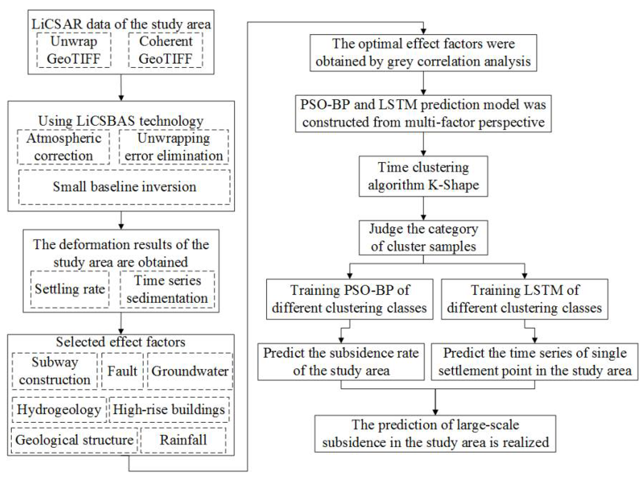
First, the LiCSBAS method was used to obtain the subsidence data for the main urban area of Kunming. According to the obtained subsidence data, the data were clustered using the time-series clustering K-shape algorithm. Next, the influence of hydrogeology, geological structure, fault, groundwater, rainfall, high-speed railway construction, and high-rise building data on urban land subsidence was analyzed. Thirdly, the PSO-BP neural network algorithm was constructed for the clustered subsidence point data from the perspective of multiple factors to predict the annual subsidence of the main urban area of Kunming from 2018-03 to 2021-02. Finally, the LSTM neural network was employed to predict the fluctuation in the subsidence sequence deformation of each subsidence point from the perspective of multiple factors. Finally, the large-scale land-subsidence prediction in the main urban area of Kunming was performed. The method flow is demonstrated in Figure 3.

2.2.1. LiCSBAS Technology to Obtain Subsidence Information

The LiCSBAS (small-baseline subset within LiCSAR) analysis method is an open-source InSAR time-series analysis method based on the LiCSAR [1] product, which is an automated Sentinel-1 InSAR processor. LiCSBAS can effectively solve large-scale monitoring that requires a significant amount of processing time and can effectively control the atmospheric delay error and phase-unwrapping error. It is particularly suitable for the acquisition of large-scale urban land-subsidence deformation information. According to Equation (1), the LiCSBAS method decomposes the interference phase to obtain the deformed phase:
φ φ topo + φ def + φ atm + φ flat + φ noise
where φtopo is the terrain phase affected by the DEM error; φdef is the deformation phase in the radar line of sight (LOS); φatm is the atmospheric delay phase; and φnoise is the flat phase. When the other phases are removed, φ can be obtained [40].
The principal steps of the LiCSBAS method are as follows. First, the LiCSAR product related to the area of interest is downloaded, and the external GACOS product is used to perform atmospheric correction for tropospheric noise [41]. Next, the overall interference quality check and loop-closure-phase difference are adopted to eliminate errors in the interference pair, and to identify and discard factors that would degrade the results. Subsequently, the interferometric pairs after atmospheric correction and unwrapping error are applied for small-baseline subset inversion to obtain the displacement time-series and rates. Next, the rate standard deviations (STD) and a noise pixel masking index are estimated based on multiple noises. Finally, the time series is spatiotemporally filtered to reduce residual noise, and the filtered time series and velocity are derived.
In the experiment, the Sentinel-1 radar image LiCSAR product processed from March 2018 to February 2021 was selected, and the LiCSBAS method was used to obtain the land-subsidence information in the main urban area of Kunming. It is expected to be used as the crucial index data for subsequent subsidence prediction.

2.2.2. K-Shape Algorithm for Clustering

K-shape is a new time-series clustering algorithm. K-shape relies on the SBD distance metric and the time-series shape extraction method to efficiently generate time-series clusters. It is based on an iterative refinement process similar to that used in K-means. Through this iterative process, K-shape minimizes the sum of squared distances and manages to produce clusters that are homogeneous (similarity of observations within clusters) and well separated (differences in observations from different clusters), and scales linearly with the number of time series. The algorithm can be used to efficiently compare sequences and computes centroids under zoom, translation, and translation invariance. K-shape is a non-trivial example of K-means. Compared with similar attempts in the literature [42,43], its distance measurement and centroid calculation method make K-shape the only scalable method that is significantly better than K-means [25]. At the same time, compared with the CLARA algorithm proposed by Gabriella Milone and Germana Scepi in 2011 [44], both K-shape and CLARA algorithms can be clustered according to shape and are suitable for processing large data sets. K-shape focuses more on to the shape of the time series, rather than the simple shape.
In each iteration, the K-shape algorithm performs two steps: (1) In the assignment step, the algorithm works by comparing each time series with all the computed centroids and assigning each time series to the closest; and (2) in the refinement step, the cluster centers are updated to reflect the changes in cluster membership in the previous step until there is no change in cluster membership or the maximum number of iterations allowed is reached. In the assignment step, K-shape depends on the SBD distance metric of Formula (2). In this paper, a brief overview of the specific flow of the K-shape algorithm is provided, and the detailed algorithm flow is detailed in [25] (Equation (2)).
S B D ( x , y ) = 1 max w ( C C w ( x , y ) i = 1 m x i · i = 1 m y i )
where x = ( x 1 , , x m ) and y = ( y 1 , , y m ) represent two time series, respectively. C C w ( x , y ) = c 1 , , c w is the cross-correlation measure of time series x and y . S B D ( x , y ) takes the value between 0 and 2, and 0 represents the complete similarity of the time series.
In the refinement step, the K-shape relies on the formula (Equation (3)) centroid calculation method; we use SBD, which determines the optimal offset x i P k for each.
μ k = arg max μ k μ k T · ( I 1 m O ) T · x i P k · ( I 1 m O ) · μ k μ k T · μ k
where the maximum value μ k * represents the square similarity of all the other time series; I is the identity matrix; O is a matrix of all ones; k is the number of clusters to be generated.
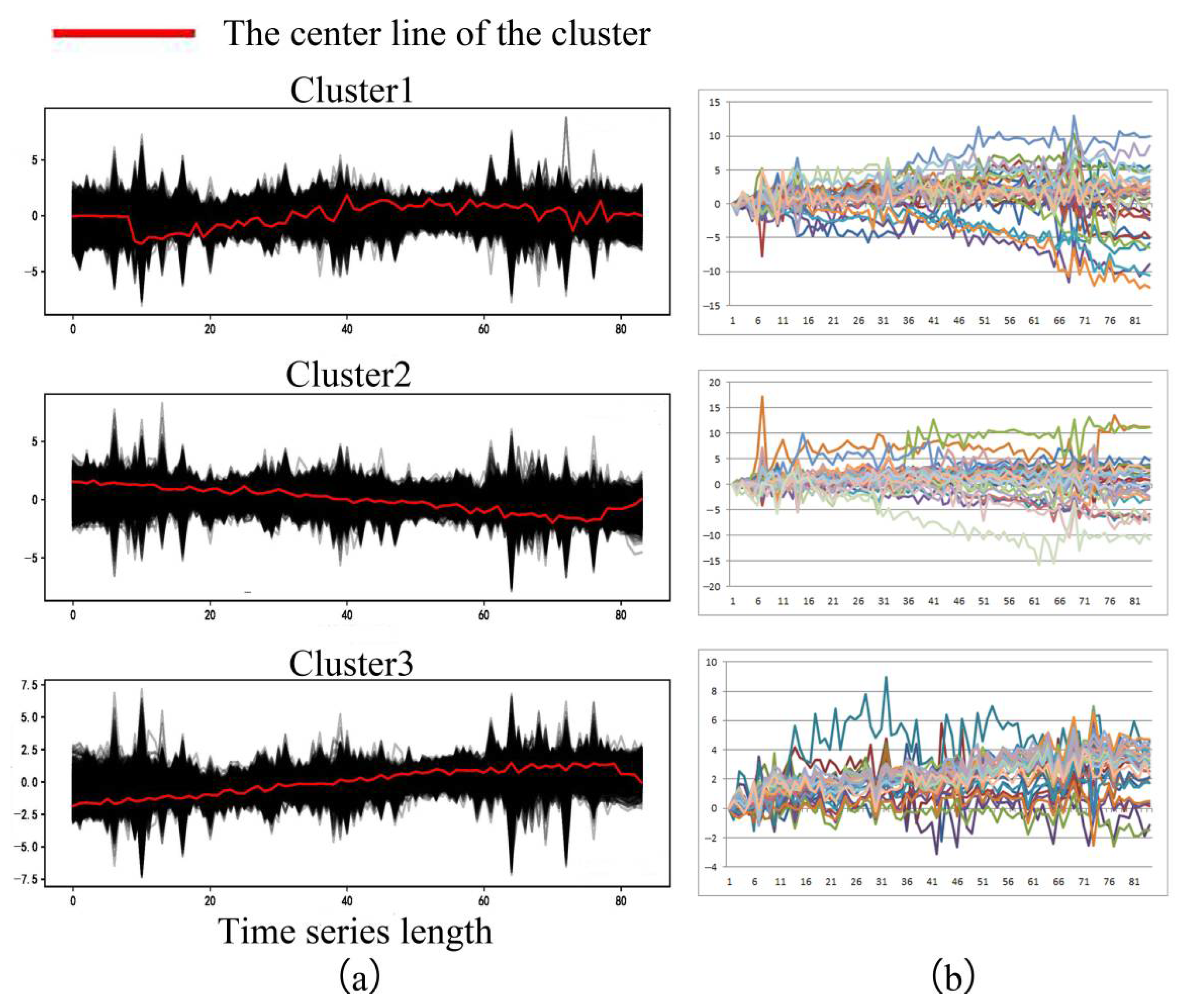
The K-shape clustering algorithm was used in this study to cluster the 40,901 subsidence data points in the main urban area of Kunming obtained by the LiCSBAS method. Furthermore, the value of the number of clusters k was determined according to the elbow diagram. In other words, the intra-cluster error variance SSE (sum of squares for error) was taken as the objective function to divide the clusters. Finally, the subsidence data of the same time series shape were clustered. According to the elbow diagram, the clustering was the most reasonable when k = 3. The 40,901 subsidence data points in the main urban area of Kunming were divided into three clusters, with subsidence data points in each cluster of 7951, 11,928, and 21,022, respectively.

2.2.3. Grey Relational Analysis

The purpose of grey correlation analysis is to quantitatively reflect the correlation between the target variable and the influencing factors so as to screen out the main factors among the numerous influencing factors. The focus of grey correlation analysis is on ranking the correlations between sequences by calculating correlations instead of calculating specific correlation values between sequences. Therefore, the criterion for selecting factors for the grey relational degree is which input factors are determined according to the order of the relational degree when the number of inputs to the prediction model is fixed, rather than whether the relational degree is higher than a certain relational value. According to the error of the prediction model under different input numbers, the input factor of the model is determined. The principle is to convert the statistical data corresponding to the variable factors in the system into geometric curves. Grey relational analysis holds that the closer the curve geometry, the greater the relational degree. The factor corresponding to the curve is the main factor dominating the development trend of the system. The steps in grey correlation calculation are presented in [45].
In the experiment, the target variable represents the average annual sedimentation rate. The data from the hydrogeology, geological structure, fault, groundwater, rainfall, subway construction, and high-rise buildings are X m , which represents the m th influencing factor, and x m ( n ) , which represents the mth influencing factor of the nth subsidence point. Each impact factor is expressed as a series of variables (Equation (4)):
{ X 1 = { x 1 ( 1 ) , x 1 ( 2 ) , , x 1 ( n ) } X i = { x i ( 1 ) , x i ( 2 ) , , x i ( n ) } X m = { x m ( 1 ) , x m ( 2 ) , , x m ( n ) }
Then find the correlation coefficient (Equation (5)):
γ [ x 0 ( k ) , x i ( k ) ] = min i min k | x 0 ( k ) x i ( k ) | + τ max i max k | x 0 ( k ) x i ( k ) | | x 0 ( k ) x i ( k ) | + τ max i max k | x 0 ( k ) x i ( k ) |
In the formula, τ take the common value of 0.5.
The correlation between X 0 and X i is obtained according to the formula (Equation (6)):
γ ( X 0 , X i ) = 1 n k = 1 n γ [ x 0 ( k ) , x i ( k ) ]
In the experiment, 2000 pieces of data were randomly selected from the clustered data to conduct grey correlation analysis using SPSSAU, an online Statistical Product and Service Solutions (SPSS) analysis software. Additionally, the qualitative influencing-factor faults, subway construction, and high-rise buildings were quantitatively processed through a buffer analysis covering the study area. Finally, the distance to the fault, subway, and high-rise buildings was determined, as shown in Figure 4. Figure 4a represents the distance from the fault; Figure 4b represents the distance from the subway; Figure 4c represents the distance from the high-rise building.According to the grey correlation analysis, the relationship between the influencing factors (hydrogeology, geological structure, groundwater, rainfall, distance from faults, subway, and high-rise buildings) and target variables (the average annual ground subsidence of the main urban area of Kunming) was obtained, and the cause of its subsidence is discussed.

2.2.4. Neural Network Algorithm

  • PSO optimization of BP neural network algorithm
The BP neural network is a common branch of the neural network, which applies the error back-propagation between the predicted value and the actual value to update the weights and biases in the BP neural network. The relationship between the input parameter x and the output value y can be expressed as Equation (7).
y = f ( w x + b )
where w and b represent the weight matrix and bias vector from adjacent layers, respectively, and f represents the activation function [29].
The neural BP network learning algorithm has shortcomings, such as its slow convergence speed, the ease with which it falls into local minima, and its difficult-to-determine network structure. The particle swarm algorithm was employed to optimize the weights and thresholds of the BP neural network. The PSO algorithm was first proposed by American electrical engineer Eberhart and social psychologist Kennedy in 1995, based on flocks of birds foraging [29]. In the PSO algorithm, the population is a set of particles, and each particle represents a potential solution to the problem, encoded by the weights and biases of the hidden and output layers in the BP neural network. Each particle has its own velocity and position vector. The evaluation index of the performance of each particle is the fitness function based on the prediction error of the BP neural network. The individual particle searches its search space and obtains the position where the fitness function reaches the maximum value, which is called the individual optimal position. Regarding all the particles, the position that the highest fitness function of a single particle can reach is called the global optimal position. The new velocity and position vector for each particle is updated with the current velocity, the individual optimal position, and the global individual optimal position. The detailed update rules are presented in [28].
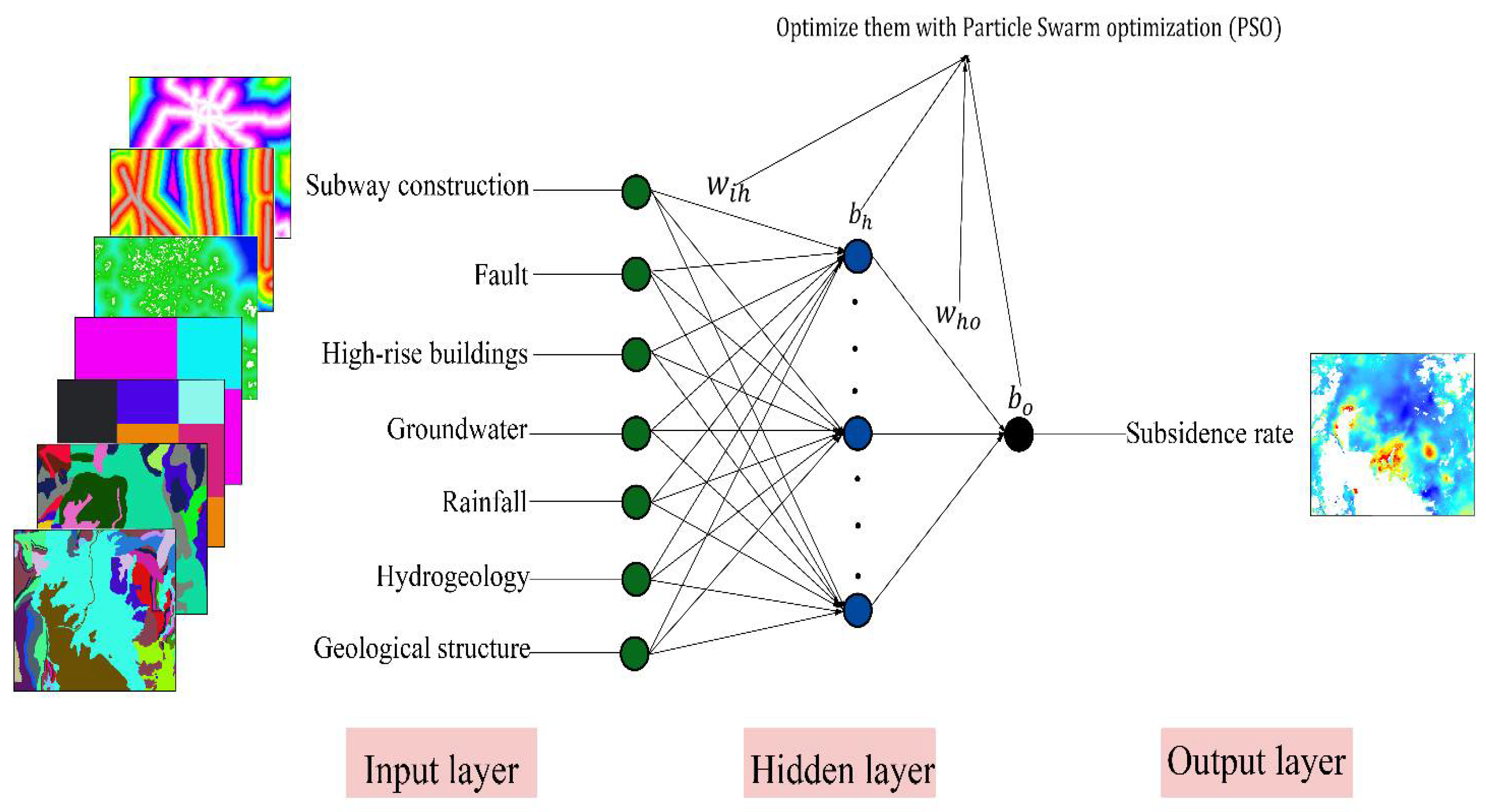
In this study, the BP neural network optimized by PSO was divided into three layers: input layer, hidden layer, and output layer. The multi-factor PSO-BP prediction model constructed in this experiment is illustrated in Figure 5. The input layer contains seven neurons: hydrogeology, geological formation, groundwater, rainfall, distance to fault, high-speed rail, and high-rise buildings. The output layer contains one neuron, which is the settling rate. The activation functions of the hidden layer and input layer were selected as tansig and purelin, respectively, and the training function was selected as trainlm. According to multiple experiments, the training parameters of the PSO-BP model under different clusters were obtained. The mean squared error (MSE) was selected as the loss function, which can be obtained by Equation (8). The PSO-BP neural network is trained from the training set until the performance on the training and validation sets does not significantly improve [32]. If either of these two criteria is met, the training process of the PSO-BP neural network is stopped. One criterion is that the mean squared error (MSE) of the training set is below 1 × 10⁻⁸. Another criterion is that the MSE of the validation set fails to decrease in 20 consecutive iterations, so as to prevent overfitting in the training process. The three types of data set divided by K-shape clustering were divided into training set, validation set, and test set, of which the training set and the validation set accounted for 40% and 10%, respectively. Different PSO-BP models were trained, and the remaining 50% comprised the test set. The mean squared error (MSE) was used to evaluate the performance of the analysis and prediction. The detailed mathematical expression is expressed in Equation (8). Finally, the subsidence rate of the main urban area of Kunming in 2018–2021 was predicted.
M S E = 1 N i = 1 N ( x i y i ) 2
where N represents the number of samples; x i represents the actual annual subsidence rate; and y i represents the predicted annual subsidence rate.
  • LSTM neural network algorithm
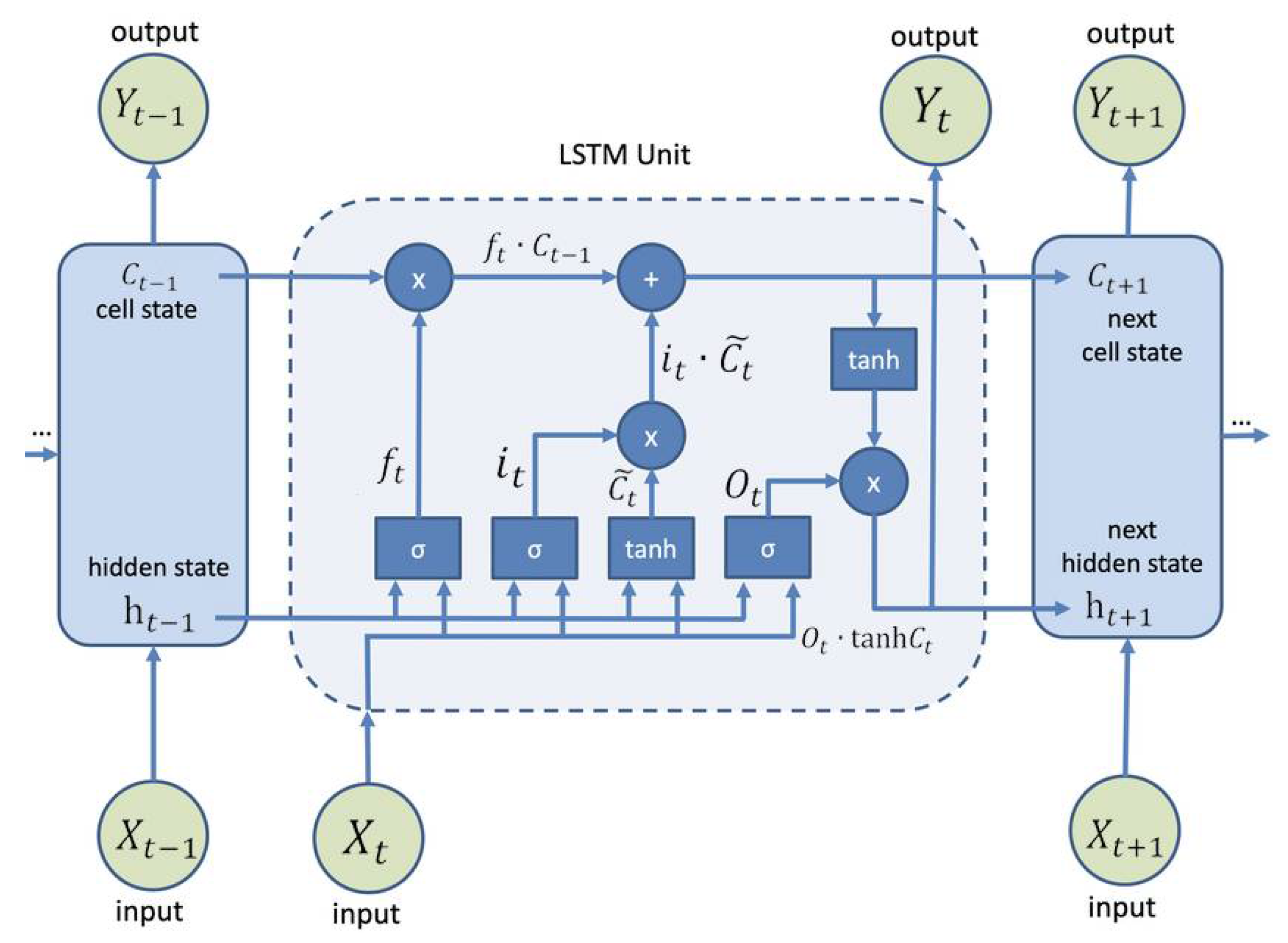
LSTM networks are special types of recurrent neural network that learn long-term dependent information [46]. If the gap between the current predicted position and the relevant information keeps increasing, the simple recurrent neural network may lose its ability to learn information from such a long distance away, and the performance of the recurrent neural network is also limited. For cases such as this, in 1997, Hochreiter and Schmidhuber proposed the long short-term memory (LSTM) network [47]. Unlike the single-loop body structure, the LSTM network structure is a special network structure with a three-“gate” (forgetting gate, input gate, and output gate) structure. For many problems, LSTM networks have achieved considerable success, and they have been widely used for sequence modeling tasks [48]. Most of the current recurrent neural networks are implemented through the LSTM network structure. The basic LSTM neural network structure is shown in Figure 6. The value σ represents the sigmoid function, and its output is between 0 and 1; tanh is the hyperbolic tangent function, and its output is between −1 and 1; h t 1 represents the output of the previous cell; and X t represents the input of the current cell.
The first stage of the LSTM neural network decides whether to forget or remember information in the cell state. The calculation formula of the forgetting gate is as follows (Equation (9)):
f t = σ ( W f · [ h t 1 , X t ] + b f )
where σ is a sigmoid activation function, f t is the forgetting gate, h t 1 is the output at time t − 1, and X t is the input vector at time t. The values W f and b f represent the weight vector and bias vector of the forget gate, respectively. If the output value of f t is close to 0, this means that the previous data have been forgotten; however, if it is close to 1, this does not mean that the previous data have been remembered.
The second stage of the LSTM neural network determines which new data are stored in the cell state. Achieving this requires two steps: first, the sigmoid layer decides which information needs to be updated, and the tanh layer generates a vector, which is an alternate candidate value C ˜ t for updating, which is added to the cell state. Second, by combining the two pieces of data, the model creates new values to update the cell state. The formula for calculating the input gate is as follows (Equations (10) and (11)):
i t = σ ( W i · [ h t 1 , X t ] + b i )
C ˜ t = tanh ( W C · [ h t 1 , X t ] + b C )
where σ is a sigmoid-shaped activation function, i t is the input gate, W i and b i represent the weight vector and bias vector of the input gate, respectively, and W C and b C represent the updated weights and biases, respectively.
In the third stage of the LSTM neural network, the old cell state C t 1 is updated by f t and i t . The values C ˜ t and C t 1 are multiplied by f t to remove redundant information. The new cell state C t is obtained by updating the past state C t 1 . This is calculated as follows (Equation (12)):
C t = f t · C t 1 + i t · C ˜ t
The final stage of the LSTM neural network decides what to output. First, we run a sigmoid layer to determine which part of the cell state will be output. Next, we process the cell state through tanh (to obtain a value between −1 and 1) and multiply it with the output of the sigmoid gate; consequently, we output only the part of the output we determined. This is calculated as follows (Equations (13) and (14)):
O t = σ ( W O · [ h t 1 , X t ] + b O )
h t = O t tanh ( C t )
where h t represents the new output value, O t is the output gate, and W O and b O represent the weight vector and bias vector of the output gate, respectively.
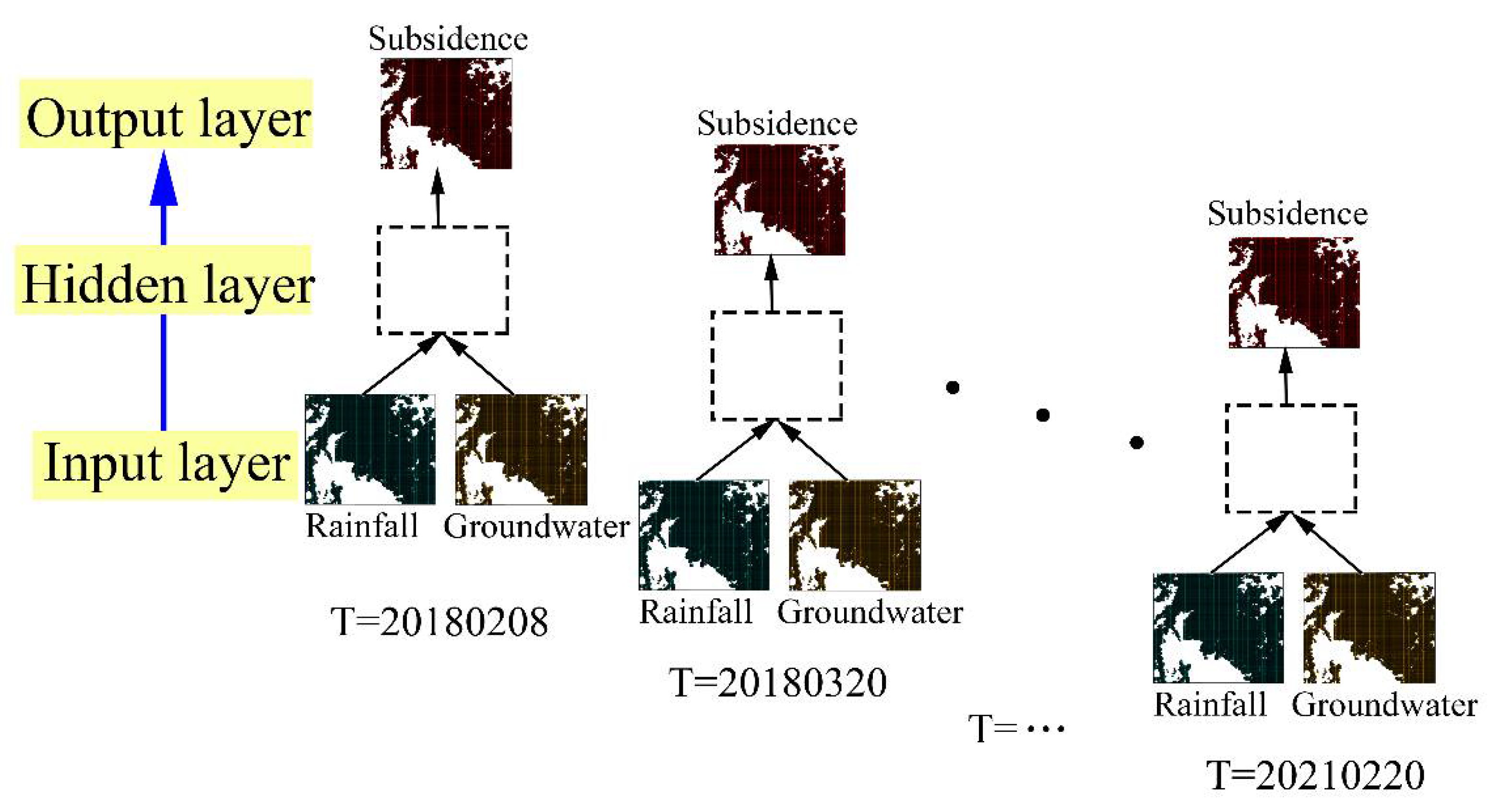
In this study, the multi-phase subsidence deformation of the same subsidence point has no relationship with the distribution distance of subways, high-rise buildings, river systems, and faults. It is mainly associated with the rainfall and groundwater data in the corresponding time period of the month. Furthermore, the deformation of the time-series subsidence of a single subsidence point is predicted using the LSTM neural network algorithm. The rainfall and groundwater data in the corresponding time period of the month are used as the input layer, and the subsidence is the output layer. The multi-factorial LSTM prediction model constructed in this experiment is presented in Figure 7. Following the length of the historical sequence L, a new data set was created through a sliding window and divided into a training set and a test set, suggesting that the first 76 periods should be selected as training samples and the last 10 periods used as verification and test samples. The time errors were lower than the multi-step prediction. Therefore, the single-step prediction method was preferred in this paper to build the network model, implying that the time step was 1 [49]. The various training parameters were set as follows: the hidden layer node was 50 layers; the training times of Cluster 1, Cluster 2, and Cluster 3 were set to 1400, 1000, and 1500 times, respectively; the batch size was set to 45; the rectified linear unit (ReLU) function was selected as the neuron activation function; and the learning rate η was 0.01. The learning rate was adjusted according to the changes in the MAE index of the test set, and the parameters were updated using the adaptive moment estimation (Adam) algorithm. Compared with other optimization methods, the overall performance of the Adam algorithm in practical applications is better, and the loss function adopts the mean absolute error. The root mean square error and mean absolute error were selected to evaluate the prediction accuracy of the LSTM neural network (Equations (15) and (16)). Finally, the time-series deformation and subsidence of a single subsidence point in the main urban area of Kunming from 2018 to 2021 were predicted.
R M S E = t = 1 N ( y t y ˜ t ) 2 N
M A E = 1 N | t = 1 N y t y ˜ t |
where y t and y ˜ t are the observed and predicted values of the subsidence at time t, respectively, and N is the number of experimental datasets.

3. Results

3.1. InSAR Land-Subsidence Deformation Results

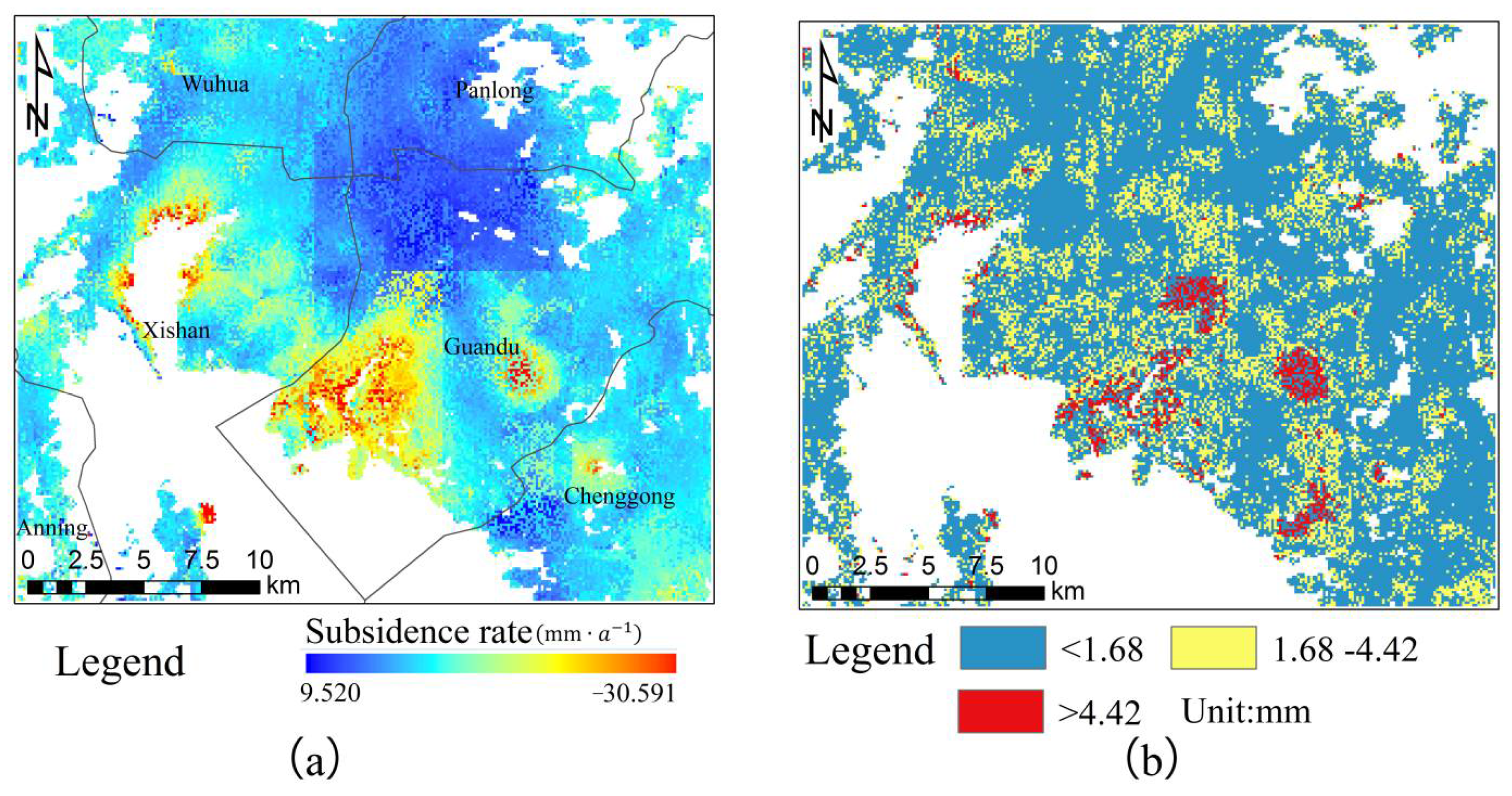
The deformation rate of the main urban area of Kunming from 2018 to 2021 is illustrated in Figure 8a. From 2018 to 2021, the maximum land-subsidence rate in the main urban area of Kunming was −30.591 mm a 1 . There are four significant subsidence areas in the main urban area of Kunming City. They are unevenly distributed along Dianchi Lake. Except for the area of Xiaobanqiao Street, the former subsidence center, the newly added settlement area A and the existing settlement area B have developed into new settlement centers in the main urban area of Kunming, distributed along Dianchi Lake, indicating that the early isolated subsidence centers are gradually developing into regional subsidence zones. The subsidence area A is mainly located in the Rongchuang–Xinhe–Wangjiadui community area in Kunming, Xishan District, showing a “three-core” distribution. The maximum subsidence is located in Rongchuang, with the maximum subsidence rate of −25.46 mm a 1 . Subsidence area B is the largest subsidence center in the main urban area of Kunming and continues to expand from south to north to the city center. Here, the subsidence is more severe. This area is located in Liujia Village, Caojiaqiao, Niuqiao Village, and the Dianchi Exhibition Center, in the Guandu District. In the area of Sijia Community–Luoya Community–Wangjia Village and Longma Community, the largest subsidence is located near Dianchi Lake, on Huizhan North Road, with a subsidence rate of −28.01 mm a 1 . Subsidence area C is located in the Yangfu Community–Guangwei Community–Xinjing Community area, and Xiaobanqiao Street, in the Guandu District. The subsidence center is located in Guangwei Community. The subsidence trend is gradually increasing from north to south, and the subsidence near Xiaobanqiao Street has a weakening trend. The largest subsidence in the region is located in the Guangwei community, with a subsidence rate of −15.34 mm a 1 . Subsidence area D is located in the Daluoyang community and Xiaoluoyang community, and in Luoyang Street, in the Chenggong District. The largest subsidence in this area is located in the Daluoyang community, with a subsidence rate of −12.65 mm a 1 . There may be a tendency toward further subsidence. There are many sedimentation funnels in the study area, and the three-dimensional surface sedimentation rate is shown in Figure 8b.

3.2. K-Shape Time Clustering Results

Figure 9a illustrates the clustering results of the 40,901 time-series subsidence data points obtained by the K-shape algorithm, which were clustered into three categories. Due to the presence of a large amount of data in each category, it was not easy to observe the subsidence time series. Thus, 30 records were extracted from each of the three categories, with the subsidence time series presented in Figure 9b.

3.3. Grey Relational Analysis Results and Analysis

3.3.1. Grey Relational Analysis Results

The grey relational analysis was performed on the clustered data, and the results obtained are provided in Table 3. As revealed in the table, the seven types of influencing factor selected from the three clusters of data were highly correlated with the subsidence rate, and the correlation results were all greater than 0.8. This suggested that the seven selected types of influencing factor were suitable for subsequent multi-factorial model construction.

3.3.2. Relationship between Influencing Factors and Land Subsidence

  • The Influence of Urban Construction on Surface Deformation
In recent years, the construction of large-scale commercial districts, high-rise buildings, and subways has become one of the essential factors of urban development affecting urban surface deformation. Figure 10a shows the superimposed result of the vector data from the large commercial districts and high-rise buildings extracted by POI (point of interest) and the high-resolution Google image, as well as a partial enlarged image. It can be seen from the partially enlarged image that the vector data from the large-scale commercial districts and high-rise buildings proposed by POI overlap with high-resolution Google images, and all the extracted vector data of the large-scale commercial districts and high-rise buildings are consistent with the real situation, thus proving the data’s reliability and validity. Consequently, we performed an overlay analysis with the subsidence rate obtained by the LiCSBAS technique in the large commercial districts and high-rise buildings, as shown in Figure 10b. The analysis demonstrated the presence of large commercial districts and high-rise buildings within a certain range of the subsidence area. However, this does not indicate that subsidences will inevitably occur where large-scale commercial districts and high-rise buildings are present. The large-scale commercial areas and high-rise buildings had the largest subsidence within 200–600 m. This is due to the fact that the loads of high-rise buildings and large-scale commercial areas are transferred to the foundation soil through their foundations, which changes the original stress state in the foundation soil layer and generates additional stress on the foundation, resulting in soil deformation and regional subsidence. The major subsidence areas in the study area are concentrated in Xishan District and Guandu District. As the technological, cultural, and commercial centers of Kunming, the development of large-scale commercial areas and high-rise buildings is essential. After an on-the-spot investigation, the subsidence areas were found to be located in large-scale commercial areas and high-rise buildings. During the peak period of architectural development, there were several projects under construction such as Kunming Sunac and Dianchi Houhai, as well as the Dianchi Convention and Exhibition Center, Wanda Plaza, and other projects. Meanwhile, the demand is increasing. In addition to the impact of large commercial areas and high-rise buildings on the surface deformation of the main urban area of Kunming, it can be seen from Figure 10c that the surface deformation of the main urban area of Kunming was affected by the construction of the subway. Table 4 provides the construction and operation time of each subway line. The table implies that the subsidence area is located around the subway; subsidence area A is located near the first phase (L9) of Metro Line 6, and subsidence area D is located near the first phase (L1) of Metro Line 1. The operation of these two subway lines began in 2012. It can be demonstrated that the vibration generated during the operation of the subway would cause damage to the ground. Subsidence has an effect. Metro Line 4 (L7) runs through subsidence area C and is under construction from 2018 to 2020. The second phase (L5) of Metro Line 2 (L5) and Line 5 (L8) runs through subsidence area B. Owing to the excavation of deep foundation pits and underground structure works during the construction of the subway, the excavation of the soil will be difficult when unloading the soil. The movement of the surface soil into the mining surface, the deformation of the enclosure structure of the deep foundation pit, and the overall subsidence of the underground structure all cause surface subsidence. Consequently, most of the subsidence areas are located around the subway. Compared with the subway lines already in operation, the subway lines under construction are more likely to cause subsidence in the surrounding land, and the subsidence is most severe 400–1200 m from the subway under construction.
  • Influence of geological structure and faults on surface deformation
Quaternary lacustrine facies and delta facies loose sedimentary layers are widely developed in the study area, mainly lacustrine facies silt and soft clay, interspersed with multiple layers of silt, peat, and lignite. According to the drill holes, the Quaternary has complex sedimentary facies transitions, both longitudinally and laterally. The northeastern part is dominated by delta facies deposition; the southwestern part is dominated by lacustrine facies, accounting for more than 1/2 of the section thickness, with 7–20 layers (27 at most) of peat and lignite, with a single layer thickness of 0.5–26.6 m. The sedimentary thickness gradually increased from 100 m to more than 500 m from the northeast to the southwest, and the cohesive soil layer also increased. In the profile, in addition to the weak clay and silty clay layers (mostly lacustrine facies) intercalated with sand, gravel or gravel layers (mostly alluvial or lacustrine facies), there are also sand, pebble, and gravel layers. There are weak clay, silty clay or peat soil layers [34]. As shown in Figure 11a, the main geological structures of the four land-subsidence areas in the main urban area of Kunming are all lacustrine sedimentary layers, consisting of sand, clay, and peat soil, with a thickness of 62 m. The physical and mechanical properties of the soil layer are shown in Table 5. The water content (w) in the settlement area is generally 13%~45% (up to 60%), the void ratio (e) is 0.1~1.1 (up to 3.8), and the compressibility (α1-2) is 0.092~0.866 MPa−1 (maximum 1.793 MPa−1), indicating that the settlement area has the characteristics of self-weight compaction, soft structure, low-degree consolidation, high compressibility, and high water content, resulting in land subsidence. The settlement range is wide and the settlement rate is high. The subsidence area near the surface is mainly soft soil, the mechanical properties of the soft soil are poor, the construction of the soft soil distribution area is difficult, and the deformation of and damage to houses and roads are common. The results revealed that subsidence areas A and B are located at the edge of Dianchi Lake, where groundwater is abundant and the sedimentary layer is relatively soft. The construction of subways, high-rise buildings, and other large-scale projects can lead to sedimentary layer subsidence. Concurrently, as shown in Figure 11b, subsidence area A is located at the intersection of the Pudu River fault zone (north section) (F1), the Chenggong–Fumin fault zone (F2), and the Machang–Xianjie (F5) fault, and it runs through the subsidence zone, exhibiting a cross-intersecting shape. The Chenggong–Fumin fault zone (F2) runs through subsidence zone B, and the Heilongtan–-Guandu fault zone (F3) is nearby, demonstrating a “V”-shaped fault interaction in the study area (Figure 11b). For the main urban area of Kunming, the impact of the fault on the surface deformation is more significant. If there is a fault, the stability of the soil structure is damaged and the land subsidence is aggravated. Heilongtan–Guandu fault zone (F3) and Baiyi–Hengchong fault (F4) are nearby, although no fault zone runs through subsidence zones C and D.
  • Influence of Hydrogeology and Groundwater Exploitation on Surface Deformation
Land subsidence requires certain soil geological hydrogeological conditions and stress-transition conditions. Regarding the hydrogeological conditions, confined aquifers with abundant water that are suitable for long-term exploitation are frequently present in systems with relatively loose water-bearing systems. Within a certain range of this mining layer, it is beneficial to land subsidence if its top and bottom have relatively thick under-consolidated or normally consolidated cohesive soil layers. From the perspective of stress transformation in the soil layer, the fluctuating and substantial reduction in the confined water level has become the basic premise for the expansion of land subsidence. The main hydrogeological types in the study area, including metamorphic rock fissure water, loose rock pore water, clastic rock fissure water, and carbonate rock fissure water, are displayed in Figure 12a. The results suggested that except for subsidence area A, which is located in the fissure water of metamorphic rocks, most of the other subsidence areas are located in the pore water of loose rocks and lack rich amounts of water. The study area is dominated by surface water, and the groundwater extraction in Kunming is mainly composed of karst water, pore water, and fissure water, which is generally used for urban living-, industry, and other purposes. The amount of groundwater exploitation is relatively large, the buried depth of the groundwater table in the subsidence area is shallow, and the burial depth of the pore water is generally 0–5 m. Affected by the shallow depth of the groundwater level, problems such as pit-wall collapse, water, and sand gushing may occur during the excavation of foundation pits, and the improper exploitation of pore water can easily cause land subsidence.
According to the water-level monitoring data in Yunnan Province, as shown in Table 6 (see Figure 12b for the groundwater exploitation sites in the corresponding blocks), the large-scale concentration and over-exploitation of groundwater has led to a continuous decline in the water level of a wide range of hot water; the decline rate is increasing, and a falling funnel has gradually formed. In the early 1980s, the burial depth of the hot water level was generally 4~6m, and the water inflow volume of a single well was 1000~1750 m3/d. However, the current water level is generally lower than the water level when the well was completed, and the average burial depth of the water level has increased to 11~25 m3/d. m; the maximum decline value is more than 35 m, the average decline rate for many years is 1.80 m/a, and the maximum is 4.59 m/a [34]. Land subsidence is closely related to the decline in groundwater over time. The evolution of land subsidence is a process involving the excessive exploitation of groundwater, the continuous decline in water level, and continuous formation and expansion. After controlling the amount of groundwater extraction, the groundwater level can gradually rise, and the land-subsidence rate also decreases or even stops. Since the data related to groundwater exploitation could not be obtained, we used the groundwater data released by NASA to obtain groundwater data for the same number of days and analyzed the four randomly selected time-series settlement points D1, D2, D3 and D4, as shown in Figure 12b. The analysis results are shown in Figure 12c. As can be seen from the figure, the cumulative subsidence values of the four time-series subsidence points show seasonal changes with groundwater, which is consistent with the high correlation between the groundwater and subsidence we obtained through the grey correlation degree.
  • The influence of rainfall on the surface deformation
Kunming features distinct dry and wet seasons in terms of time distribution, and its annual rainfall is 1450 mm. The rainy season is from May to October, and the rainfall in this period accounts for about 85% of the total for the whole year. The dry season lasts from November to April of the following year, and the rainfall during this period only comprises about 15% of the annual total. As mentioned above, the main urban area of Kunming is mainly composed of a lacustrine sedimentary layer, which comprises sand, clay, and peat soil. The subsidence area is mainly soft soil near the surface, which is prone to collapse and deformation under the action of rainfall. In this study, a superposition analysis of the annual rainfall and the subsidence area in the corresponding time range, from 2018 to 2021, was performed to explore the influence of rainfall on the surface deformation in Kunming. It was discovered that the average annual rainfall is more likely to lead to land subsidence in the range of 109–117mm. Furthermore, the time-series points P1, P2, P3, and P4 (as shown in Figure 12b) were randomly selected within the four subsidence regions, as presented in Figure 13. The four selected subsidence points exhibit nonlinear subsidence and have a good correlation with rainfall. The deformation time-series fluctuates with the change in rainfall; the main outcome is that the deformation variable increases with the rainfall, forming a markedly accelerated process. Simultaneously, the effect of rainfall on land subsidence is temporary, and the surface deformation will gradually tend toward the original normal consolidation and subsidence process when the rainfall stops. The four subsidence points, P1, P2, P3, and P4, settled faster and displayed seasonal changes. The P2 and P3 subsidence points settled the fastest, and their maximum subsidence values were −64.45 mm and −60.75 mm, respectively. This was due to the fact that the two subsidence points were subsided by the combined action of subways, high-rise buildings, and rainfall.

3.4. Construction and Demonstration Application of Subsidence Prediction Model

3.4.1. Multi-Factorial PSO-BP Model to Predict Sedimentation Rate Results

The best prediction-model training parameters obtained by the constructed multi-factor PSO-BP model for the three categories of data after several adjustments are presented in Table 7. The training-set data from different categories (Cluster 1, Cluster 2, and Cluster 3) were predicted by the corresponding constructed PSO-BP models for the validation and test sets, and their corresponding mean squared errors (MSE) were as follows: 1.519, 1.465; 1.419, 1.441; and 1.485, 1.494, respectively. Specifically, the smaller the MSE, the more the prediction model described, and the better the accuracy of the experimental data. Meanwhile, there was no over-fitting phenomenon. The final predicted sedimentation rate of the main urban area of Kunming from 2018–2021 is illustrated in Figure 14a. The PSO-BP model constructed by using this paper can effectively predict a large area of urban land subsidence, and its predicted subsidence area is consistent with the results of the InSAR monitoring of the subsidence area. As revealed by calculating the error between the predicted subsidence rate and the actual InSAR monitoring rate (Figure 14b), the areas with a prediction error of less than 1.68 mm account for the largest total in the whole study area, and the areas with a prediction error greater than 4.42 mm are mainly concentrated near the subsidence area, especially the C subsidence area, which features the largest error. By calculating the MSE of the predicted and monitored values for the whole study area as 4.821 mm, according to the DZ/T 0154-2020 “Specification for Ground Subsidence Measurement” issued by the Ministry of Natural Resources of China, the deformation accuracy of the SBAS-InSAR is ±10 mm. Among the 24,540 predicted subsidence-rate points, there are 24,432 deformation accuracies greater than 0 and less than ±10 mm, accounting for about 99.5%; the deformation accuracy is higher than ±10 mm in 108 cases, accounting for about 0.5%. This implies that the prediction accuracy meets the measurement specification requirements. Thus, the effectiveness of the PSO-BP algorithm for predicting the land-subsidence rate in a large urban area was verified.

3.4.2. Multi-Factorial LSTM Model to Predict Time-Series Subsidence Results

The constructed multi-factorial LSTM model was used to predict the last ten periods of any time-series sedimentation data in each of the three types of data, and the results are provided in Figure 15. The root mean square error (RMSE) of the three types of data (Cluster 1, Cluster 2, and Cluster 3) are 0.445, 1.475, and 1.468 mm, respectively; the mean absolute errors (MAE) are 0.319, 1.214, and 1.167 mm, respectively; the absolute error ranges are 0.007~1.030, 0~3.001, and 0.401~3.679 mm, respectively. It can be observed that the root mean square error and mean absolute error of the three types of data are very small, and the maximum absolute error of the three types of data is 3.679 mm, which satisfies the DZ/T 0154-2020 “Ground Subsidence Measurement Specification” issued by the Ministry of Natural Resources of China, with an SBAS-InSAR deformation Accuracy ±10 mm. Therefore, it was verified that the multi-factorial LSTM model can be used to predict the subsidence of the time series.

4. Discussion

4.1. Influence of the Accuracy of InSAR Monitoring Results on the Prediction Model

The large-scale urban land-subsidence prediction method proposed in this paper from the perspective of multiple factors is mainly based on the use of the subsidence rate and time-series data obtained by InSAR technology to perform the corresponding prediction. It can be demonstrated that the accuracy of the InSAR monitoring results directly affects the final prediction accuracy. Due to the lack of a contemporaneous leveling survey and GPS survey data, the accuracy of the monitoring data in this paper cannot be accurately evaluated. To this end, the annual subsidence rate data of the study area obtained in different historical periods were collected and compared with the annual subsidence rate obtained by the method in this paper, as listed in Table 8. This comparison suggests that the subsidence rates of the five selected subsidence areas, including Guangwei Village, Xiaobanqiao, and Yuhu Village, are in good agreement with the leveling data and the data obtained through InSAR. Thus, a field investigation on the subsidence area obtained above was conducted to understand whether the monitoring results were in line with the actual situation. It was revealed that the impact of subsidence on buildings and foundations can be clearly observed in the subsidence area, as presented in Figure 16.
In summary, LiCSBAS technology was used as a means of obtaining early large-scale urban land-subsidence monitoring data in this study. The monitoring results can be used to effectively control the atmospheric delay and phase unwrapping, while the monitoring data accuracy is in line with the actual situation. It acts as a late prediction model.

4.2. The Advantages and Disadvantages of the Constructed Multi-Factorial Prediction Model Compared with Existing Prediction Models

The urban land-subsidence prediction model we constructed from a multi-factorial perspective is different from that used by previous researchers, who simply used monitoring data as the main factor. Although its subsidence prediction accuracy is high, it only plays a fitting role. So far, a few researchers have tried to predict from a multi-factorial perspective in other fields [6], although they could not effectively predict time-series data. Meanwhile, large-scale subsidence prediction could not be achieved. The multi-factor PSO-BP model we constructed can effectively predict the land-subsidence rate in large cities. Moreover, the multi-factorial LSTM model we constructed can accurately capture and predict the subsidence deformation of serial time series. Furthermore, the K-shape time-series clustering algorithm was introduced in this paper to manage large-scale forecasting. Compared with the prediction accuracy without clustering, as exhibited in Table 9, the prediction accuracy after clustering is slightly higher than before clustering. If the training samples are gradually reduced so that they cannot fully learn the large-scale sedimentation rate, the prediction accuracy without clustering is lower than after K-shape clustering.
There are still some deficiencies in the multi-factorial prediction model described in this paper. For example, the selected influencing factors were shown to be highly correlated with subsidence through grey relational analysis. Whether the size has an impact on the final prediction accuracy remains to be demonstrated. The data from each cluster were obtained, and our experiment solved the drawback that the previous prediction model could not accurately capture or predict the sedimentation deformation of the sequence time series. However, although we obtained a suitable parameter selection for the data under each cluster, the number of iterations for each time-series subsidence point was different, and it was impossible to use the unified parameters to predict the entire region time-series subsidence. Only the multi-factorial LSTM we constructed point is trained to predict each point. It can undoubtedly increase the handling workload, which will also be studied in follow-up research.

4.3. Analysis of InSAR Processing Limits and Error Control

In this article, we described the use of LiCSBAS technology to obtain the urban land-subsidence deformation rate in the study area, which is limited by the LiCSAR product released by COMET, a project of the Centre for Seismological and Volcanic Structure Observation and Modelling of the UK Environmental Research Council (NERC). For the research area we selected, we found that some data were missing from the coherence map obtained under the descending orbit of the research area by querying the LiCSAR product; therefore, although we could use the LiCSAR product under the ascending orbit to obtain the subsidence rate along the radar’s line of sight, we could not obtain the settling rate in the vertical direction. At the same time, LiCSBAS technology is more suitable for processing Sentinel data, and it does not easily process ALOS PALSAR, TerraSAR-X-1, or other data.
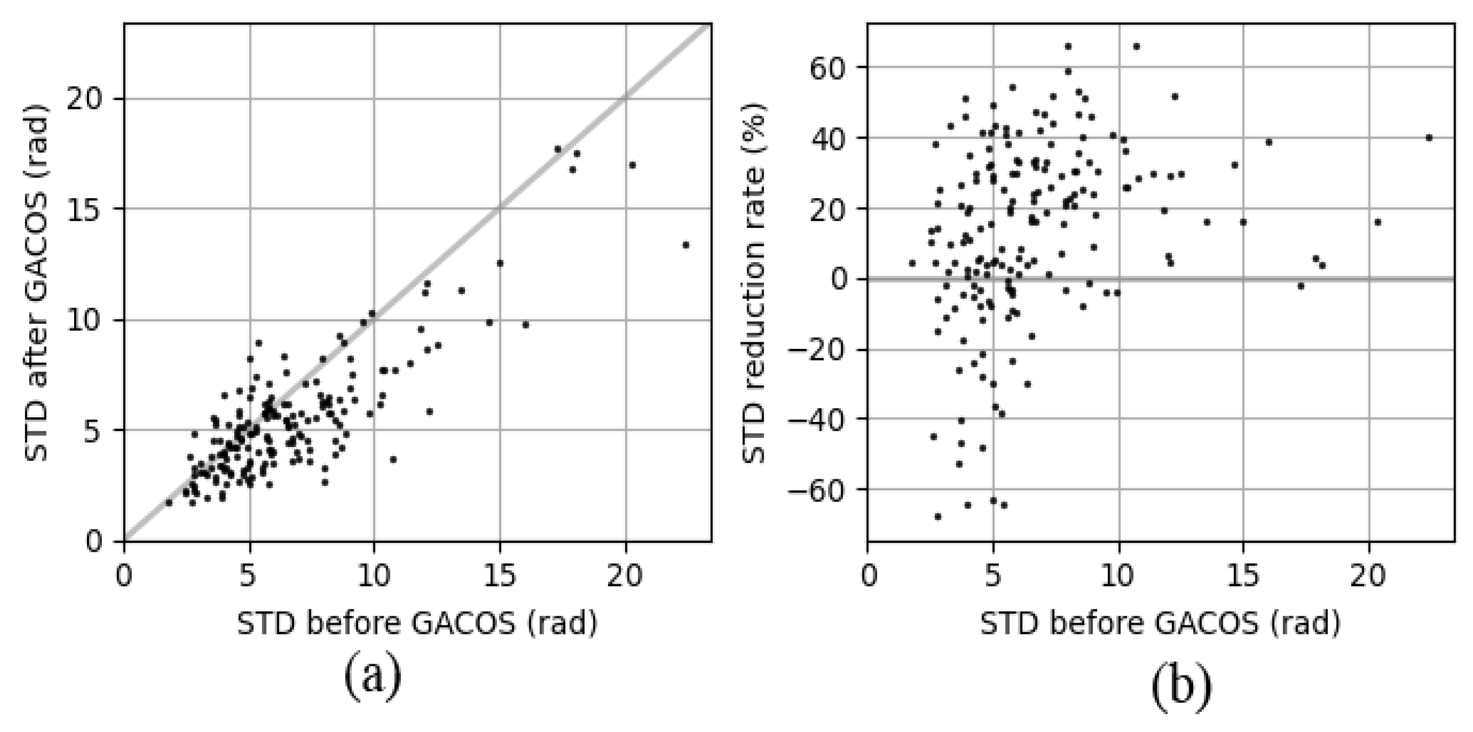
Atmospheric delay error and phase unwrapping error are two of the main errors in InSAR deformation inversion, and improving them can effectively improve the final monitoring accuracy. The atmospheric delay error is corrected to reduce its effect. At present, there are two main methods of atmospheric correction: (1) In the time series, the data set composed of multiple interferograms is filtered to estimate the phase of the atmospheric effects and remove them [50]; and (2) external data, such as GPS data, meteorological observations, or other on-board sensor data, are used for calibration [51]. The above methods have their respective advantages and disadvantages, and there is currently no general method to eliminate atmospheric imagery. In this experiment, we chose to introduce GACOS products for atmospheric correction, and used the overall interference-quality inspection and loop-closure phase to eliminate the unwrapping errors [17]. Figure 17 shows the phase standard deviation correlation diagrams of 189 pairs of interferograms in the main urban area of Kunming before and after the GACOS correction. From Figure 17a, it can be seen that the phase standard deviation after the GACOS correction was significantly lower than before the correction, and the maximum-phase standard deviation after the correction reduced from 8.0 rad to 2.7 rad. From Figure 17b, it can be seen that the rate of change of the STD before and after the correction was significantly reduced in 73.4%, and the negative impact after the correction accounted for 26%, a total of 47 pairs. The gray line indicates that the phase STD and its rate of change remained unchanged before and after the correction. It can be seen that using GACOS to correct tropospheric atmospheric delay has a certain effect.
The quality inspection of the overall interferometric pairs in the study area corrected by the GACOS atmospheric delay product did not detect interferometric pairs with low coherence and fewer effective pixels. The interferometric pairs that satisfied the quality inspection were checked for loop-closure phase, and the threshold was set as 1.5 rad, and we generated an interference-pair space-time baseline distribution diagram, as shown in Figure 18. The blue is the space-time baseline generated after the overall interference-pair-quality inspection, and the red is the unqualified interference pair after the loop-closure-phase inspection, which needs to be eliminated.

4.4. Error Source Control Analysis and the Shortcomings of This Method

4.4.1. Error Source Control Analysis

The main limitations of the method in this paper are the various image factors in the input layer of the neural network. In order to ensure the accuracy of the influencing factors input by the input layer and control their errors, in Section 2.1.3, which describes the general situation of the study area, through the discussion of the causes of urban land subsidence in the study area by existing scholars, the factors affecting land subsidence were obtained. On this basis, through the correlation analysis of the above-mentioned influencing factors in Section 3.3.1, it was proven, from a quantitative point of view, that the influencing factors selected in this paper have a high correlation with urban land subsidence, and that each type of influencing factor selected has a high degree of correlation, above 0.8. In general, if the correlation between the input layer (influencing factors) and the output layer (urban land-subsidence rate) of the neural network is greater than 0.6, a neural network model can be established for prediction. This paper effectively guarantees the accuracy of influencing factors and controls their errors from both qualitative and quantitative perspectives.

4.4.2. Shortcomings of This Method

In this study, a particle swarm optimization–back propagation (PSO-BP) neural network algorithm was constructed from a multi-factorial perspective to predict urban land subsidence, and then the LSTM neural network was used to predict the sequence deformation of the urban land subsidence from a multi-factorial perspective. The fluctuation in the land subsidence eventually produced a large-scale urban land-subsidence prediction. However, there the following two problems remain: (1) We established buffers with a certain width range for the subways, large commercial areas, high-rise buildings, and faults to quantitatively process them. The specific width of the buffer zone was a given number of meters, and the prediction accuracy obtained was the best, which remains to be further verified by future research. (2) Since large-scale hydrogeological, geological structure, and fault data are classified data, they are not made public in China; therefore, higher and larger-scale data could not be obtained. The accuracy of the predictions will be further improved if these predictions can be made using larger-scale hydrogeological, geological structure, and fault data.

5. Conclusions

Existing neural network models are over-reliant on historical subsidence data for urban land-subsidence prediction and cannot accurately capture or predict fluctuations in the sequence deformation. Regarding large-scale urban land-subsidence prediction, the improper selection of training samples directly affects the final results and the prediction accuracy. Therefore, this paper proposed a subsidence prediction method based on a neural network algorithm from a multi-factorial perspective, given the shortcomings of the previous neural network model in urban land-subsidence prediction. Additionally, a K-shape clustering algorithm was adopted to select a large range of training samples. Finally, the subsidence rate and time-series subsidence of the main urban area of Kunming from 2018 to 2021 were predicted to explore the use of high-precision urban land-subsidence prediction methods. The conclusions are as follows.
(1) The LiCSBAS method can effectively monitor the urban land subsidence in the main urban area of Kunming. A new time-series method, LiCSBAS, was used to monitor the maximum land-subsidence rate of −30.591 mm a 1 in the main urban area of Kunming from 2018 to 2021. There are four significant subsidence areas in the main urban area of Kunming City, which are unevenly distributed along Dianchi Lake. The results revealed that land subsidence is more likely to occur within 200–600 m of large commercial areas and high-rise buildings, within 400–1200 m of the subway currently under construction, and within 109–117 mm of the average annual rainfall. The existence of faults will destroy the stability of the soil structure and increase the land subsidence. The hydrogeology, geological structure, and groundwater also have a certain influence on the land subsidence of the main urban area of Kunming.
(2) After clustering, the multi-factorial PSO-BP model can effectively predict large-scale urban land subsidence. The K-shape clustered data Cluster 1, Cluster 2, and Cluster 3 were predicted by the corresponding multi-factorial PSO-BP model for the validation set and test set. The corresponding mean square errors (MSE) were as follows: 1.519, 1.465; 1.419, 1.441; and 1.485, 1.494, respectively. The smaller the MSE, the better the accuracy of the prediction model in describing the experimental data. Moreover, there was no overfitting phenomenon. Among the 24,540 predicted sedimentation-rate points, 24,432 had a deformation accuracy greater than 0 and less than ±10 mm, accounting for about 99.5%; and 108 had a deformation accuracy greater than ±10mm, accounting for about 0.5%. It was demonstrated that the prediction accuracy met the requirements of the measurement specification. The prediction accuracy after clustering was slightly improved compared to the accuracy when no clustering was used.
(3) The constructed multi-factorial LSTM can effectively capture and predict fluctuations in the sequence deformation. The constructed multi-factorial LSTM model was used to predict the next ten periods of any time-series subsidence data in the three types of data. The root mean square errors (RMSE) of the three types of data (Cluster 1, Cluster 2, and Cluster 3) were 0.445, 1.475, and 1.468 mm, respectively; the mean absolute errors (MAE) were 0.319, 1.214, and 1.167 mm, respectively; the absolute error ranges were 0.007~1.030, 0~3.001, and 0.401~3.679 mm, respectively. This prediction accuracy met the requirements of measurement specifications.
(4) The results demonstrate the application of large-scale, high-precision urban land-subsidence prediction. The prediction model we constructed from the perspective of multiple factors can effectively predict the land-subsidence rate and time-series subsidence of large cities, suggesting that it can be used to perform prediction by inputting the corresponding influencing factors. Our research expands the application scope of land-subsidence prediction models from the relationship between multiple factors and subsidence. This is different from previous studies, which adopted existing monitoring data to build their models. This paper lays a foundation for large-scale urban land-subsidence prediction.
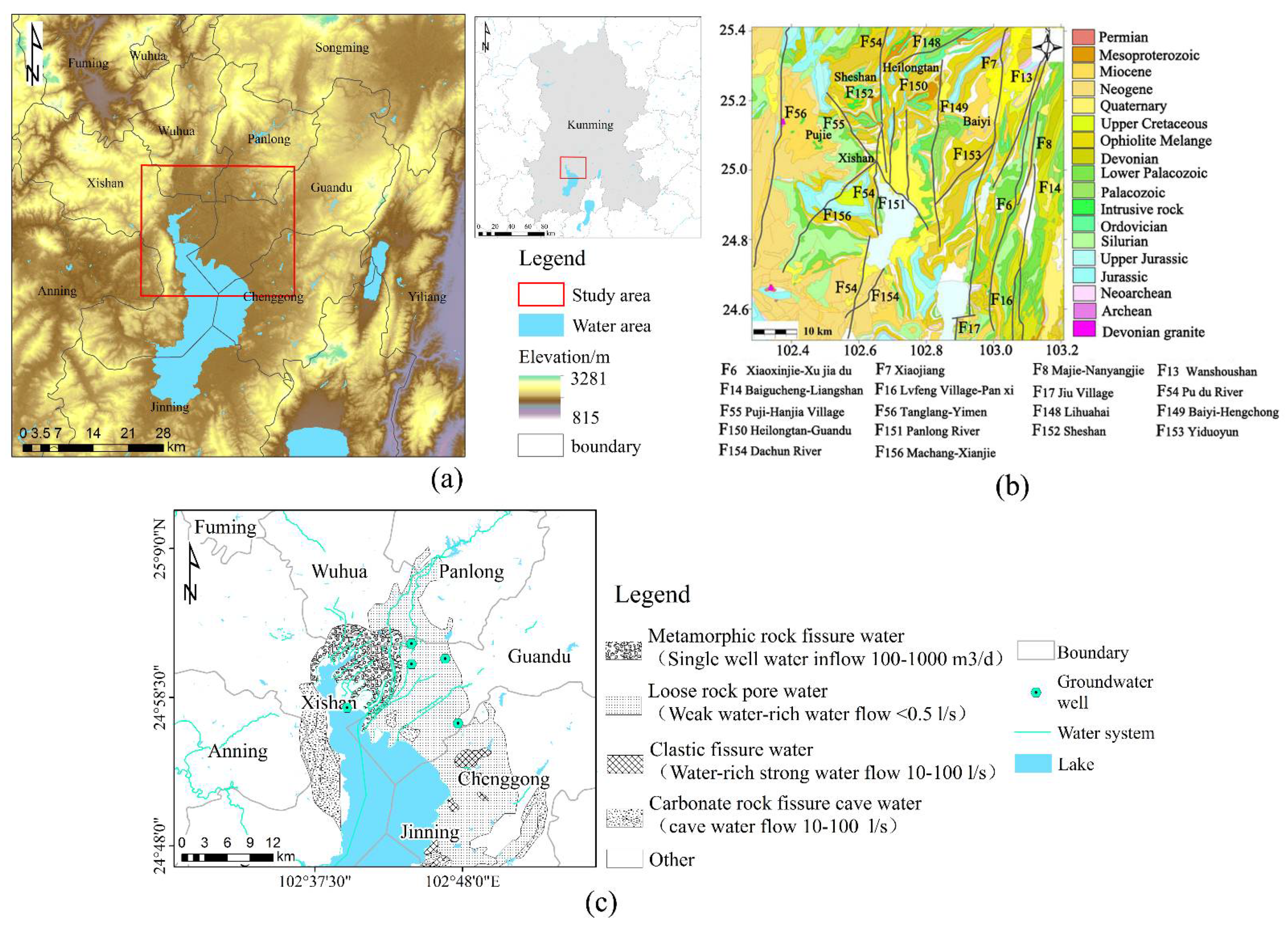
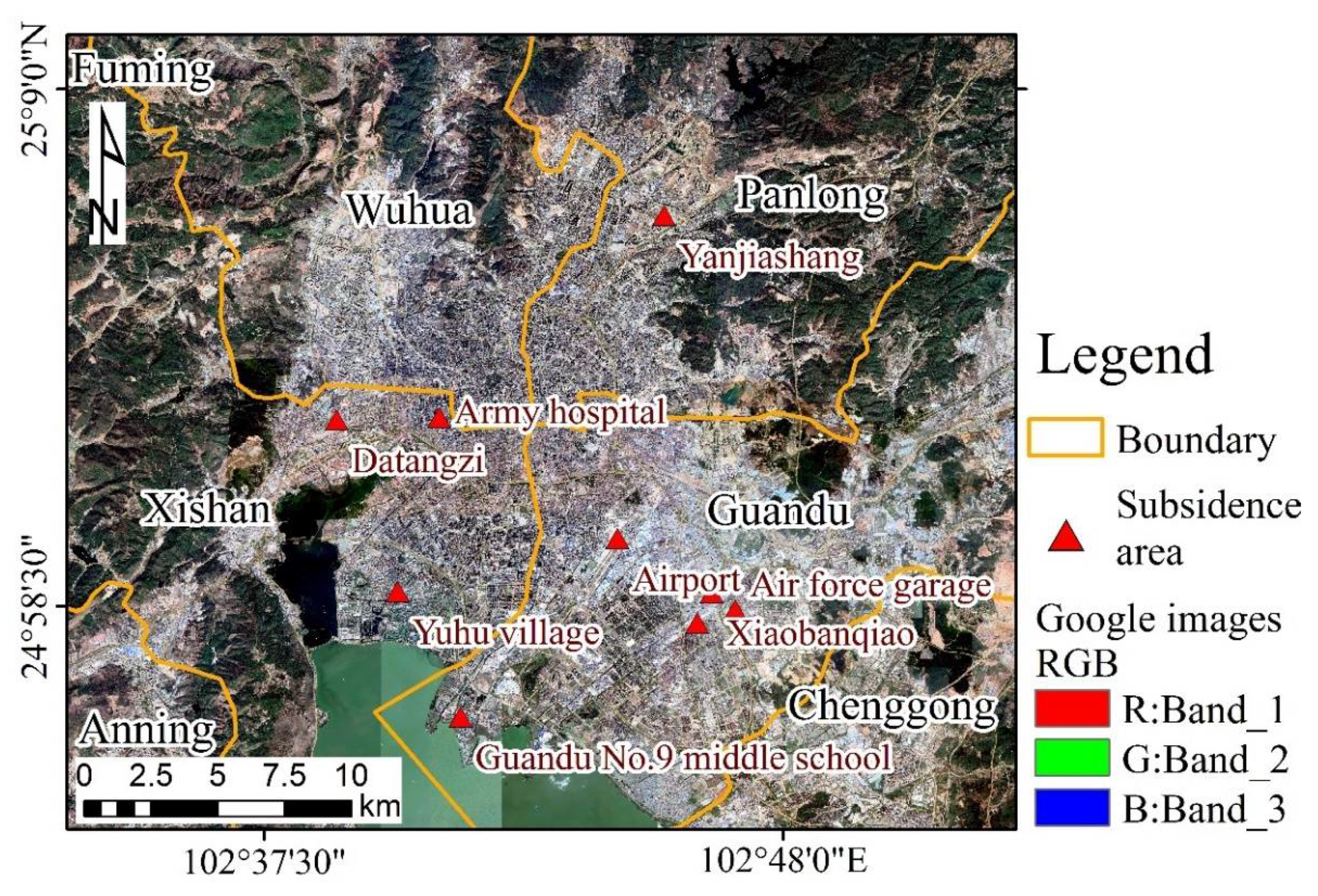
Author Contributions

D.Z. designed the experiments, performed the algorithm, and wrote the original paper. Writing—review and editing, X.Z. and Z.Z.; funding acquisition, X.Z. and Z.Z.; Z.Z. provided guidance. All authors have read and agreed to the published version of the manuscript.

Funding

This research was funded by “National Natural Science Foundation of China” (grant no. 42161067), “General Project of Applied Basic Research Program of Yunnan Province” (grant no. 2018FB078) and “Joint Foundation Project between Yunnan Science and Technology Department and Yunnan University” (grant no. 2019FY003017).

Institutional Review Board Statement

Not applicable.

Informed Consent Statement

Not applicable.

Data Availability Statement

The data presented in this study are available upon request from the corresponding author.

Acknowledgments

The authors would like to thank the anonymous reviewers for their valuable feedback on the manuscript. We would also like to thank the UK Environmental Research Council (NERC) Centre for Seismological and Volcanic Tectonic Observation and Modelling for the LiCSAR product released by COMET and the GACOS tropospheric delay correction product released by the University of Newcastle, UK.

Conflicts of Interest

The authors declare no conflict of interest.

References

  1. Zhou, Q.; Hu, Q.; Ai, M.; Xiong, C.; Jin, H. An improved GM (1, 3) model combining terrain factors and neural network error correction for urban land subsidence prediction. Geomat. Nat. Hazards Risk 2020, 11, 212–229. [Google Scholar] [CrossRef] [Green Version]
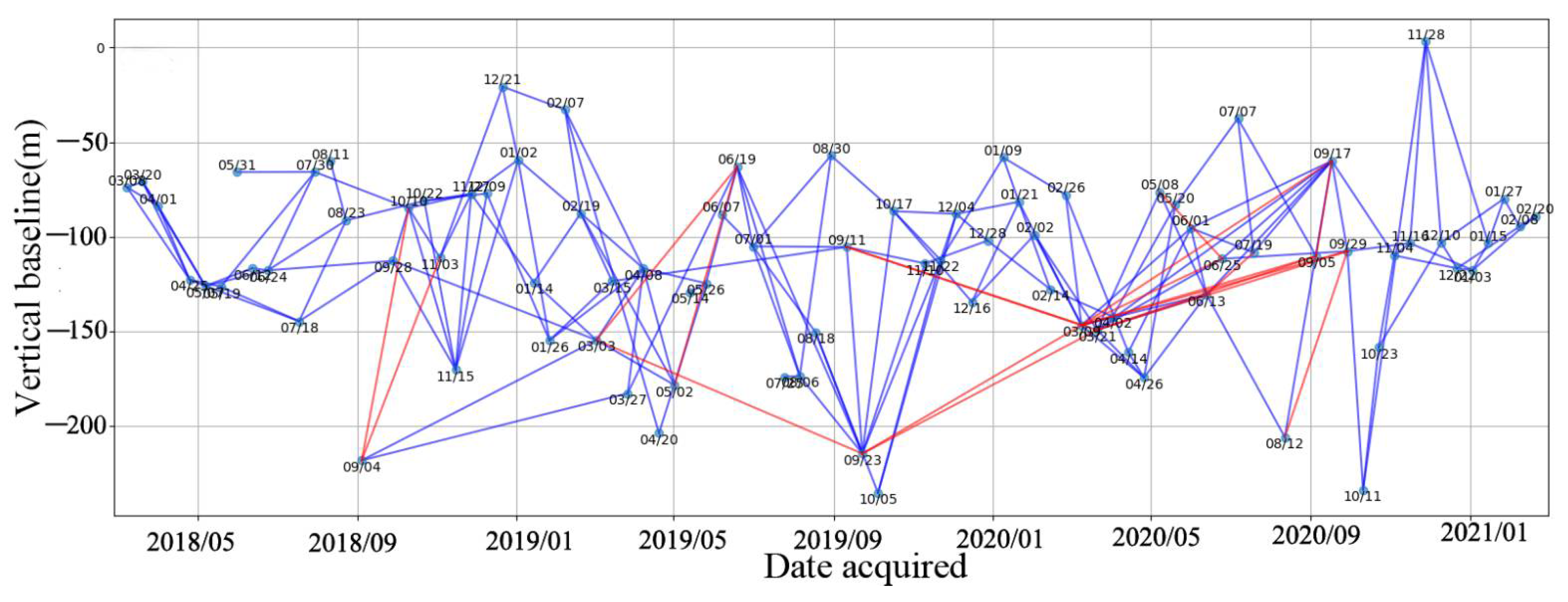
  2. Pradhan, B.; Abokharima, M.H.; Jebur, M.N.; Tehrany, M.S. Land subsidence susceptibility mapping at Kinta Valley (Malaysia) using the evidential belief function model in GIS. Nat. Hazards. 2014, 73, 1019–1042. [Google Scholar] [CrossRef]
  3. Holzer, T.L.; Johnson, A.I. Land subsidence caused by ground water withdrawal in urban areas. GeoJournal 1985, 11, 245–255. [Google Scholar] [CrossRef]
  4. Hu, R.L.; Yue, Z.Q.; Wang, L.U.; Wang, S.J. Review on current status and challenging issues of land subsidence in China. Eng. Geol. 2004, 76, 65–77. [Google Scholar] [CrossRef]
  5. Lu, N.; Hernandez, A.J.; Ramsey, R.D. Land cover dynamics monitoring with Landsat data in Kunming, China: A cost-effective sampling and modelling scheme using Google Earth imagery and random forests. Geocarto Int. 2015, 30, 186–201. [Google Scholar] [CrossRef]
  6. A’Campo, W.; Bartsch, A.; Roth, A.; Wendleder, A.; Martin, V.S.; Durstewitz, L.; Hugelius, G. Arctic Tundra Land Cover Classification on the Beaufort Coast Using the Kennaugh Element Framework on Dual-Polarimetric TerraSAR-X Imagery. Remote Sens. 2021, 13, 4780. [Google Scholar] [CrossRef]
  7. Zhu, W.; Li, W.L.; Zhang, Q.; Yang, Y.; Zhang, Y.; Qu, W.; Wang, C.S. A decade of ground deformation in Kunming (China) revealed by multi-temporal synthetic aperture radar interferometry (InSAR) technique. Sensors 2019, 19, 4425. [Google Scholar] [CrossRef] [Green Version]
  8. Hanssen, R.F. Radar Interferometry: Data Interpretation and Error Analysis; Kluwer Academic Publishers: Dordrecht, The Netherlands, 2001. [Google Scholar]
  9. Tantianuparp, P.; Shi, X.; Liao, M.; Zhang, L.; Balz, T. Landslide Monitoring in Three Gorges Area Using D-InSAR and PS-InSAR. In Proceedings of the Dragon 2 Final Results and Dragon 3 Kickoff Symposium, Beijing, China, 25–29 June 2013; Volume 704, p. 88. [Google Scholar]
  10. Dai, K.; Liu, G.; Li, Z.; Li, T.; Yu, B.; Wang, X.; Singleton, A. Extracting vertical displacement rates in Shanghai (China) with multi-platform SAR images. Remote Sens. 2015, 7, 9542–9562. [Google Scholar] [CrossRef] [Green Version]
  11. Liu, X.; Zhao, C.; Zhang, Q.; Lu, Z.; Li, Z.; Yang, C.; Liu, C. Integration of Sentinel-1 and ALOS/PALSAR-2 SAR datasets for mapping active landslides along the Jinsha River corridor, China. Eng. Geol. 2021, 284, 106033. [Google Scholar] [CrossRef]
  12. Kang, Y.; Lu, Z.; Zhao, C.; Xu, Y.; Kim, J.W.; Gallegos, A.J. InSAR monitoring of creeping landslides in mountainous regions: A case study in Eldorado National Forest, California. Remote Sens. Environ. 2021, 258, 112400. [Google Scholar] [CrossRef]
  13. Shao, X.; Ma, S.; Xu, C.; Zhang, P.; Wen, B.; Tian, Y.; Zhou, Q.; Cui, Y. Planet Image-Based Inventorying and Machine Learning-Based Susceptibility Mapping for the Landslides Triggered by the 2018 Mw6.6 Tomakomai, Japan Earthquake. Remote Sens. 2019, 11, 978. [Google Scholar] [CrossRef] [Green Version]
  14. Lazecky, M.; Perissin, D.; Bakon, M.; de Sousa, J.M.; Hlavacova, I.; Real, N. Potential of Satellite InSAR Techniques for MonitoringBridge Deformations. In Proceedings of the 2015 Joint Urban Remote Sensing Event (JURSE), Lausanne, Switzerland, 30 March–1 April 2015. [Google Scholar]
  15. Yang, K.; Yan, L.; Huang, G.; Chen, C.; Wu, Z. Monitoring Building Deformation with InSAR: Experiments and Validation. Sensors 2016, 16, 2182. [Google Scholar] [CrossRef] [PubMed]
  16. He, Y.; Xu, G.; Kaufmann, H.; Wang, J.; Ma, H.; Liu, T. Integration of InSAR and LiDAR Technologies for a Detailed Urban Subsidence and Hazard Assessment in Shenzhen, China. Remote Sens. 2021, 13, 2366. [Google Scholar] [CrossRef]
  17. Morishita, Y.; Lazecky, M.; Wright, T.J.; Weiss, J.R.; Elliott, J.R.; Hooper, A. LiCSBAS: An open-source InSAR time series analysis package integrated with the LiCSAR automated Sentinel-1 InSAR processor. Remote Sens. 2020, 12, 424. [Google Scholar] [CrossRef] [Green Version]
  18. Zhang, G.; Wu, Y.; Wang, L.; Zhang, K.; Daemen, J.J.; Liu, W. Time-dependent subsidence prediction model and influence factor analysis for underground gas storages in bedded salt formations. Eng. Geol. 2015, 187, 156–169. [Google Scholar] [CrossRef]
  19. Zhang, C.; Li, J.Z.; Yong, H.E. Application of optimized grey discrete Verhulst–BP neural network model in subsidence prediction of foundation pit. Environ. Earth Sci. 2019, 78, 1–15. [Google Scholar] [CrossRef]
  20. Li, Y.F.; Zuo, X.Q.; Ma, Y.Y.; Xiong, P.; Yany, F. Surface subsidence monitoring and prediction based on PS-InSAR technology and genetic neural network algorithm. Prog. Geophys. 2020, 35, 845–851. [Google Scholar]
  21. Chen, Y.; He, Y.; Zhang, L.; Chen, Y.; Pu, H.; Chen, B.; Gao, L. Prediction of InSAR deformation time-series using a long short-term memory neural network. Int. J. Remote Sens. 2021, 42, 6919–6942. [Google Scholar] [CrossRef]
  22. Luat, N.V.; Lee, K.; Thai, D.K. Application of artificial neural networks in subsidence prediction of shallow foundations on sandy soils. Geomech. Eng. 2020, 20, 385–397. [Google Scholar]
  23. Chen, R.P.; Zhang, P.; Kang, X.; Zhong, Z.Q.; Liu, Y.; Wu, H.N. Prediction of maximum surface subsidence caused by earth pressure balance (EPB) shield tunneling with ANN methods. Soils Found. 2019, 59, 284–295. [Google Scholar] [CrossRef]
  24. Shi, L.; Gong, H.; Chen, B.; Zhou, C. Land Subsidence Prediction Induced by Multiple Factors Using Machine Learning Method. Remote Sens. 2020, 12, 4044. [Google Scholar] [CrossRef]
  25. Paparrizos, J.; Gravano, L. k-shape: Efficient and accurate clustering of time series. In Proceedings of the ACM SIGMOD International Conference on Management of Data, Malbourne, VIC, Australia, 31 May–4 June 2015; pp. 1855–1870. [Google Scholar]
  26. Yang, F.; Cho, H.; Zhang, H.; Zhang, J.; Wu, Y. Artificial neural network (ANN) based prediction and optimization of an organic Rankine cycle (ORC) for diesel engine waste heat recovery. Energy Conv. Manag. 2018, 164, 15–26. [Google Scholar] [CrossRef]
  27. Wang, J.; Li, L.; Niu, D.; Tan, Z. An annual load forecasting model based on support vector regression with differential evolution algorithm. Appl. Energy 2012, 94, 65–70. [Google Scholar] [CrossRef]
  28. Zhao, R.; Zhang, H.; Song, S.; Yang, F.; Hou, X.; Yang, Y. Global optimization of the diesel engine–organic Rankine cycle (ORC) combined system based on particle swarm optimizer (PSO). Energy Conv. Manag. 2018, 174, 248–259. [Google Scholar] [CrossRef]
  29. Cui, Y.; Liu, H.; Wang, Q.; Zheng, Z.; Wang, H.; Yue, Z.; Yao, M. Investigation on the ignition delay prediction model of multi-component surrogates based on back propagation (BP) neural network. Combust. Flame 2022, 237, 111852. [Google Scholar] [CrossRef]
  30. Sherstinsky, A. Fundamentals of recurrent neural network (RNN) and long short-term memory (LSTM) network. Phys. D. 2020, 404, 132306. [Google Scholar] [CrossRef] [Green Version]
  31. Wei, L.; Guan, L.; Qu, L.; Guo, D. Prediction of Sea Surface Temperature in the China Seas Based on Long Short-Term Memory Neural Networks. Remote Sens. 2020, 12, 2697. [Google Scholar] [CrossRef]
  32. Crisóstomo de Castro Filho, H.; Abílio de Carvalho Júnior, O.; Ferreira de Carvalho, O.L.; Pozzobon de Bem, P.; dos Santos de Moura, R.; Olino de Albuquerque, A.; Trancoso Gomes, R.A. Rice crop detection using LSTM, Bi-LSTM, and machine learning models from sentinel-1 time series. Remote Sens. 2020, 12, 2655. [Google Scholar] [CrossRef]
  33. Chen, X.; Zhang, Y. Impacts of urban surface characteristics on spatiotemporal pattern of land surface temperature in Kunming of China. Sustain. Cities Soc. 2017, 32, 87–99. [Google Scholar] [CrossRef] [Green Version]
  34. Xue, C.D.; Li, X.; Li, B.Z.; Meng, G.T.; Li, F. Mechanism analysis of land subsidence in Kunming city area. Chin. J. Geolo. Hazard Control 2004, 3, 51–58. [Google Scholar]
  35. Li, S.; Wang, Z.; Yuan, L.; Li, X.; Huang, Y.; Guo, R. Mechanism of Land Subsidence of Plateau Lakeside Kunming City Cluster (China) by MT-InSAR and Leveling Survey. J. Coast. Res. 2020, 115, 666–675. [Google Scholar] [CrossRef]
  36. Ma, Y.Y.; Chen, Y.B.; Zuo, X.Q.; Ma, W.F.; Wu, W.H. Analysis of land subsidence in Kunming based on Sentinel-1Adata and SBAS technolog. Sci. Surv. Mapp. 2019, 44, 59–66. [Google Scholar]
  37. Mateus, P.; Catalo, J.; Nico, G. Sentinel-1 interferometric sar mapping of precipitable water vapor over a country-spanning area. IEEE Trans. Geosci. Remote Sens. 2017, 5, 1–7. [Google Scholar] [CrossRef]
  38. Lazecký, M.; Spaans, K.; González, P.J.; Maghsoudi, Y.; Wright, T.J. Licsar: An automatic insar tool for measuring and monitoring tectonic and volcanic activity. Remote Sens. 2020, 12, 2430. [Google Scholar] [CrossRef]
  39. Song, X.G.; Li, D.R.; Shan, X.J.; Liao, M.S.; Cheng, L. Correction of atmospheric effect in ASAR interferogram using GPS and MODIS data. Chin. J. Geophys. Chin. Ed. 2009, 52, 1457–1464. [Google Scholar]
  40. Hooper, A.; Zebker, H.; Segall, P.; Kampes, B. A new method for measuring deformation on Volcanoes and other natural terrains using InSAR Persistent Scatterers. Geophys. Res. Lett. 2004, 31, 1–5. [Google Scholar] [CrossRef]
  41. Yu, C.; Li, Z.; Penna, N.T.; Crippa, P. Generic atmospheric correction model for Interferometric Synthetic Aperture Radar observations. J. Geophys. Res. Solid Earth 2018, 123, 9202–9222. [Google Scholar] [CrossRef]
  42. Petitjean, F.; Ketterlin, A.; Gançarski, P. A global averaging method for dynamic time warping, with applications to clustering. Pattern Recognit. 2011, 44, 678–693. [Google Scholar] [CrossRef]
  43. Yang, J.; Leskovec, J. Patterns of Temporal Variation in Online Media. In Proceedings of the Fourth ACM International Conference on Web Search and Data Mining, Hong Kong, China, 9–12 February 2011; pp. 177–186. [Google Scholar]
  44. Gabriella, M.; Germana, S. A clustering approach for studying ground deformation trends in campania region through ps-insartm time series analysis. J. Appl. Sci. 2011, 11, 610–620. [Google Scholar]
  45. Chen, B.; Zhou, C.; Liu, Y.; Liu, J. Correlation analysis of runway icing parameters and improved PSO-LSSVM icing prediction. Cold Reg. Sci. Technol. 2022, 193, 103415. [Google Scholar] [CrossRef]
  46. Graves, A. Supervised Sequence Labelling with Recurrent Neural Networks. Stud. Comput. Intell. 2008, 2, 42–45. [Google Scholar]
  47. Hochreiter, S.; Schmidhuber, J. Long short-term memory. Neural Comput. 1997, 9, 1735–1780. [Google Scholar] [CrossRef] [PubMed]
  48. Schmidhuber, J. Deep learning in neural networks: An overview. Neural Netw. 2015, 61, 85–117. [Google Scholar] [CrossRef] [PubMed] [Green Version]
  49. Qinghao, L.I.U.; Yonghong, Z.H.A.N.G.; Min, D.E.N.G.; Hongan, W.U.; Yonghui, K.A.N.G.; Jujie, W.E.I. Time series prediction method of large-scale surface subsidence based on deep learning. Acta Geodaet. Cartograph. Sin. 2021, 50, 396. [Google Scholar]
  50. Goldstein, R. Atmospheric limitations to repeat-track radar interferometry. Geophys. Res. Lett. 1995, 22, 2517–2520. [Google Scholar] [CrossRef] [Green Version]
  51. Zhang, Z.; Lou, Y.; Zhang, W.; Wang, H.; Zhou, Y.; Bai, J. On the Assessment GPS-Based WRFDA for InSAR Atmospheric Correction: A Case Study in Pearl River Delta Region of China. Remote Sens. 2021, 13, 3280. [Google Scholar] [CrossRef]
Figure 1. (a) is the location of the study area (the map in the upper-right corner shows the location of Kunming), and the corresponding data are superimposed on those of the National Aeronautics and Space Administration (National Aeronautics and Space Administration, NASA), the Jet Propulsion Laboratory (Jet Propulsion Laboratory, JPL), and the National Imagery and Mapping Agency (NIMA), who jointly surveyed and mapped the SRTM DEM data digital elevation model; (b) is a geological map of the study area. Black solid lines represent Quaternary active faults, The copyright of this geological map comes from the College of Geology Engineering and Geomatics, Chang’an University Wu Zhu et al. [7]; (c) is a hydrogeological map of the study area.
Remotesensing 14 01803 g001
Figure 2. Location distribution of second-class level survey of the study area (relevant data superimposed on Google Image).
Remotesensing 14 01803 g002
Figure 3. Flowchart of the method (the dotted box represents the method or generated content that needed to be processed in the solid box).
Remotesensing 14 01803 g003
Figure 4. Quantitative processing of qualitative factors: (a) shows the distance to fault obtained by buffer analysis and erasure analysis; (b) shows the distance to fault obtained by buffer analysis and erasure analysis; (c) represents the distance to high-rise buildings obtained by buffer analysis and erasure analysis.
Remotesensing 14 01803 g004
Figure 5. The constructed multi-factorial PSO-BP prediction model. In the figure, w i h represents the connection weight between the input layer and the hidden layer, w h o represents the connection weight between the hidden layer and the output layer, b h represents the threshold of each neuron in the hidden layer, and b o represents the threshold of each neuron in the output layer.
Remotesensing 14 01803 g005
Figure 6. Basic structure of the LSTM model.
Remotesensing 14 01803 g006
Figure 7. The constructed multi-factorial LSTM prediction model.
Remotesensing 14 01803 g007
Figure 8. (a) Deformation rate of the main urban area of Kunming from 2018 to 2021. (b) Three-dimensional surface-subsidence-rate map of each subsidence area.
Remotesensing 14 01803 g008
Figure 9. K-shape clustering results ((a) is the result of clustering the cumulative deformation rate of the time series in the study area using the K-shape time clustering algorithm; (b) presents the extraction of 30 records from three categories to draw a subsidence time-series diagram).
Remotesensing 14 01803 g009
Figure 10. Analysis of urban construction on surface deformation: (a) is the superimposition of the results of the large-scale commercial districts and high-rise building data on a Google image, with a partial, enlarged view; (b) is the superimposition of the results of the large-scale commercial district and high-rise building data and the settlement rate; (c) is the overlaid result plot of subway data and subsidence rate.
Remotesensing 14 01803 g010
Figure 11. Geological structure and fault analysis of surface deformation: (a) is the geological structure data; (b) is the superimposed results of the fault and subsidence rate.
Remotesensing 14 01803 g011
Figure 12. Correlation analysis diagram of hydrogeology to surface deformation: (a) is a vector diagram of hydrogeology in the study area; (b) is the name of groundwater exploitation in the corresponding block (the corresponding data are superimposed on a Google image; randomly selected relative timing point locations D1, D2, D3, D4 and P1, P2, P3, P4 were superimposed on Google images). The analysis results are shown in (c).
Remotesensing 14 01803 g012
Figure 13. Analysis of the relationship between rainfall and surface deformation.
Remotesensing 14 01803 g013
Figure 14. Prediction result and prediction error of subsidence rate in LOS direction; (a) is the prediction of the subsidence rate in the main urban area of Kunming from 2018 to 2021, using the constructed PSO-BP; (b) is the error between the predicted subsidence rate and the actual monitoring rate of InSAR.
Remotesensing 14 01803 g014
Figure 15. Predicted value and true value of time-series subsidence data under different types of LSTM model.
Remotesensing 14 01803 g015
Figure 16. Field inspection map: (a) Tilt of house caused by land subsidence, (b) Due to excessive groundwater extraction, the surface subsides and deforms, eventually resulting in karst collapse, (c) Ground subsidence increases the activity of ground fissures and eventually leads to the formation of ground fissures, (d) Land subsidence will cause damage to buildings, causing building foundations to sink and houses to crack.
Remotesensing 14 01803 g016
Figure 17. Correlation diagram of phase standard deviation before and after GACOS correction: (a) is the phase difference before and after correction; (b) is the change rate of phase standard deviation before and after correction. The blue is the space-time baseline generated after the overall interference pair quality inspection, and the red is the unqualified interference pair after the loop-closure-phase inspection, which needs to be eliminated.
Remotesensing 14 01803 g017
Figure 18. Interference-pair space-time baseline distribution map.
Remotesensing 14 01803 g018
Table 1. Subsidence amount (mm) and subsidence rate ( mm a 1 ) of Kunming subsidence center.
Period1987~19941994~19981987~1998
Subsidence AreaSubsidenceRateSubsidenceRateSubsidenceRate
Guangwei village−140.1−20.0−81.3−20.3−221.4−20.1
Airforce garage−138.4−19.8−53.7−13.5−192.1−17.5
Yuhu village−44.8−6.4−50.3−12.6−95.1−8.6
Guandu No. 9 middle school *+159.2+22.7−227.1−56.8−67.8−6.2
Airport−89.5−8.1−119.4−29.9−208.9−19.0
Army hospital−186.3−16.9−96.1−24.0−282.4−25.7
Datangzi−99.5−9.0−56.9−14.2−156.4−14.3
Yanjiashang−44.5−4.0−86.5−21.6−131.0−11.9
Xiaobanqiao−111.9−16.0−124.3−31.1−236.2−21.5
Note: “+” indicates uplift; “−” indicates subsidence; “*”—the data of this measurement point do not match the overall trend of the surrounding subsidence all the time; the subsidence requires continued observation.
Table 2. Data sources and specifications.
Data NameType of DataData Resolution/ScaleData PhaseData Source
Sentinel-1A radar imageRaster5 m × 20 m2018-03–2021-02European Space Agency
LiCSAR ProductsRaster30 m2018-03–2021-02NERC and COMET
GACOSRaster90 m2018-03–2021-02University of Newcastle
SRTM DEMRaster30 m-NASA and NIMA
Google Maps imageryRaster0.2 m2021Google Earth
hydrogeologyRaster1:200,000-National Geological Archive; Institute of Geology, China Earthquake Administration
Geologic structureRaster1:200,000-
FaultRaster1:200,000-
Large business districtVector-2018-03–2021-02Bigemap map download app
High-rise buildingVector-2018-03–2021-02
SubwayVector-2018-03–2021-02
Global precipitation measurementsRaster1 km2018-03–2021-02National Aeronautics and Space Administration
GroundwaterRaster1 km2018-03–2021-02
Table 3. Grey correlation analysis results of each cluster.
Effect FactorsCorrelation Degree of Cluster 1Correlation Degree of Cluster 2Correlation Degree of Cluster 3
Subway construction0.8330.8250.869
Fault0.8300.8230.868
High-rise buildings0.8380.8270.874
Groundwater0.8420.8400.884
Rainfall0.8420.8400.884
Hydrogeology0.8360.8360.881
Geological structure0.8380.8360.869
Table 4. Timetable for construction and operation of various subway lines.
Subway LineTime (20-)
0809101112131415161718192021
Line 1 Phase I (L1)
Line 1 branch (L2)
Northwest Extension of Line 1 (L3)
Line 2 Phase I (L4)
Line 2 Phase II (L5)
Line 3 (L6)
Line 4 (L7)
Line 5 (L8)
Line 6 Phase I (L9)
Line 6 Phase II (L10)
Note: Red indicates the subway construction stage; green indicates the subway operation stage.
Table 5. Physical and mechanical properties index of Quaternary lacustrine sedimentary layer soil.
Soil TypeDensity ρ (g/cm3)Water Content w (%)Void Ratio eCompression Factor α1-2 (MPa−1)Compression Modulus Es (0.1 MPa)
Sand1.87~2.0818~350.5~0.90.499~0.09238.5~166.7
Clay1.56~2.0113~350.6~1.050.713~0.21437.7~95.2
Silty clay1.76~2.0030~450.8~1.00.866~0.13221.8~42.9
Peat1.20~1.5040~601.1~3.81.793~0.52014.54~6.5
Gravel1.95~2.3515~250.1~0.50.367455
Note: Source—Yunnan Provincial Bureau of Geology and Mineral Resources.
Table 6. Groundwater exploitation status of each block.
BlockNumber of Mining Wells (Eyes)Minimum Spacing between Production Wells (m)Cumulative Drawdown of Water Level (m)Average Drop in Water Level (m/a)
Urban area2815020.22~25.102.26
Guanshang–Jinmasi341009.18~24.881.32
Yangfangao–Paomashan212005.70~9.381.18
Haigeng sanatorium4615011.50~21.301.62
Note: According to the survey and statistical data of Yunnan Provincial Environmental Monitoring Station [34].
Table 7. Best training parameters of PSO-BP under different clusters.
ParameterCluster 1Cluster 2Cluster 3ParameterCluster 1Cluster 2Cluster 3
Learning rate0.80.80.8Learning factorc1 = c2 = 1.49445c1 = c2 = 1.49445c1 = c2 = 1.49445
Training goal0.0010.0010.001Evolution algebra202030
Number of training10,00020,00020,000PopSize202530
Factor of momentum0.60.60.6Number of hidden layers111011
Table 8. Subsidence rates of the study area at different times.
Depression AreaAverage Sedimentation Rate
1987~19941994~19982007~20102014~20162018~2021
Guangwei village−20.0 (*)−20.3 (*)−12.6
Xiaobanqiao−16.0 (*)−31.1 (*)−20.9−19.4−15.3
Yuhu village−6.4 (*)−12.6 (*)−5.1
Hewei village−2.5−25.1−26.8−24.1−16.3
Yangjia shang−4.0 (*)−21.6 (*)−6.7−4.5
Note: (*) marked as leveling data, not marked as InSAR monitoring data; “−” represents subsidence.
Table 9. Prediction accuracy before and after clustering.
Evaluation IndexNon-Use of K-ShapeUse of K-Shape
MSE4.9354.820
MAE1.4871.474
Publisher’s Note: MDPI stays neutral with regard to jurisdictional claims in published maps and institutional affiliations.