
PlumeTraP: A New MATLAB-Based Algorithm to Detect and Parametrize Volcanic Plumes from Visible-Wavelength Images


Abstract
:1. Introduction
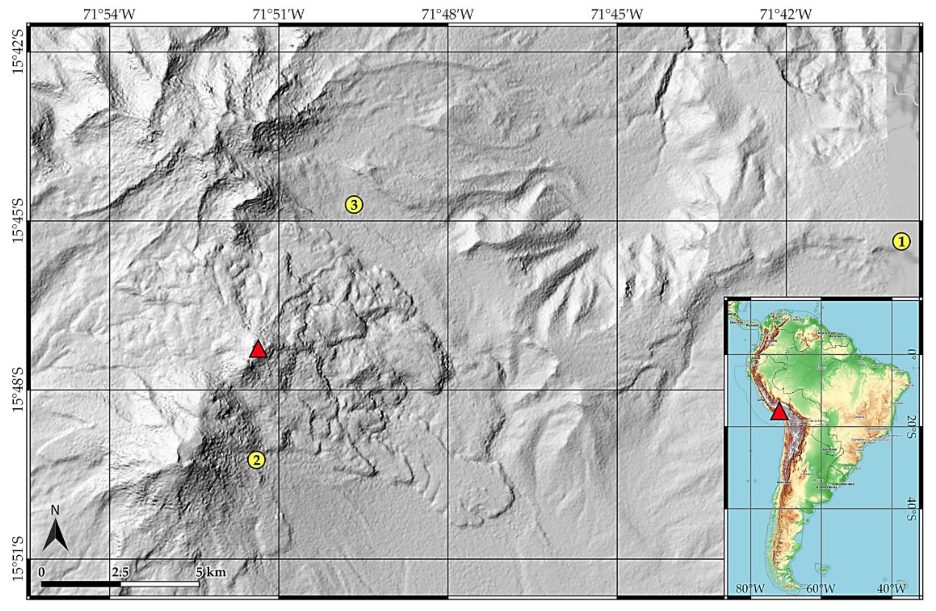
2. Field Site
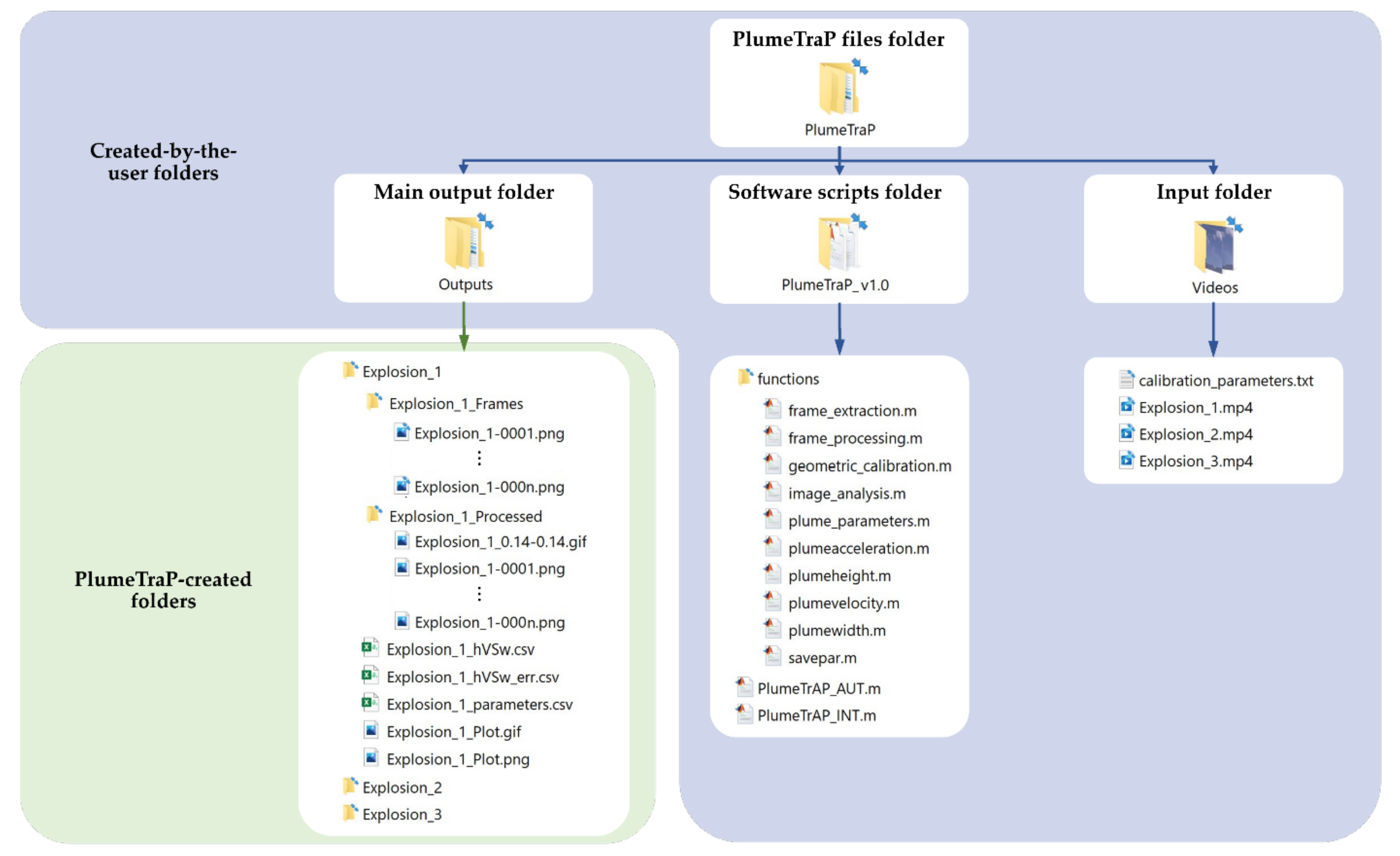
3. Methods: Structure of PlumeTraP Software
3.1. Video Analysis
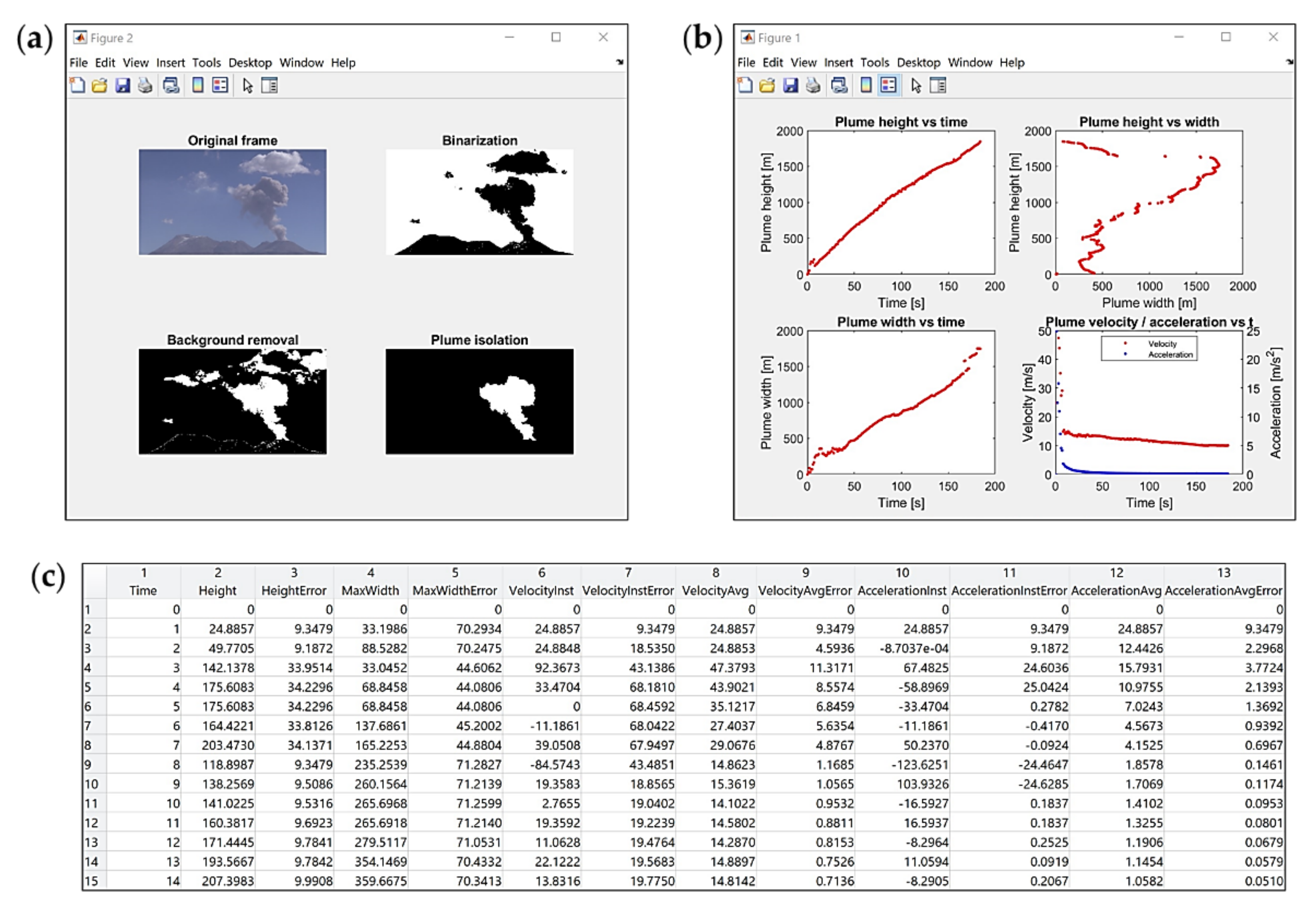
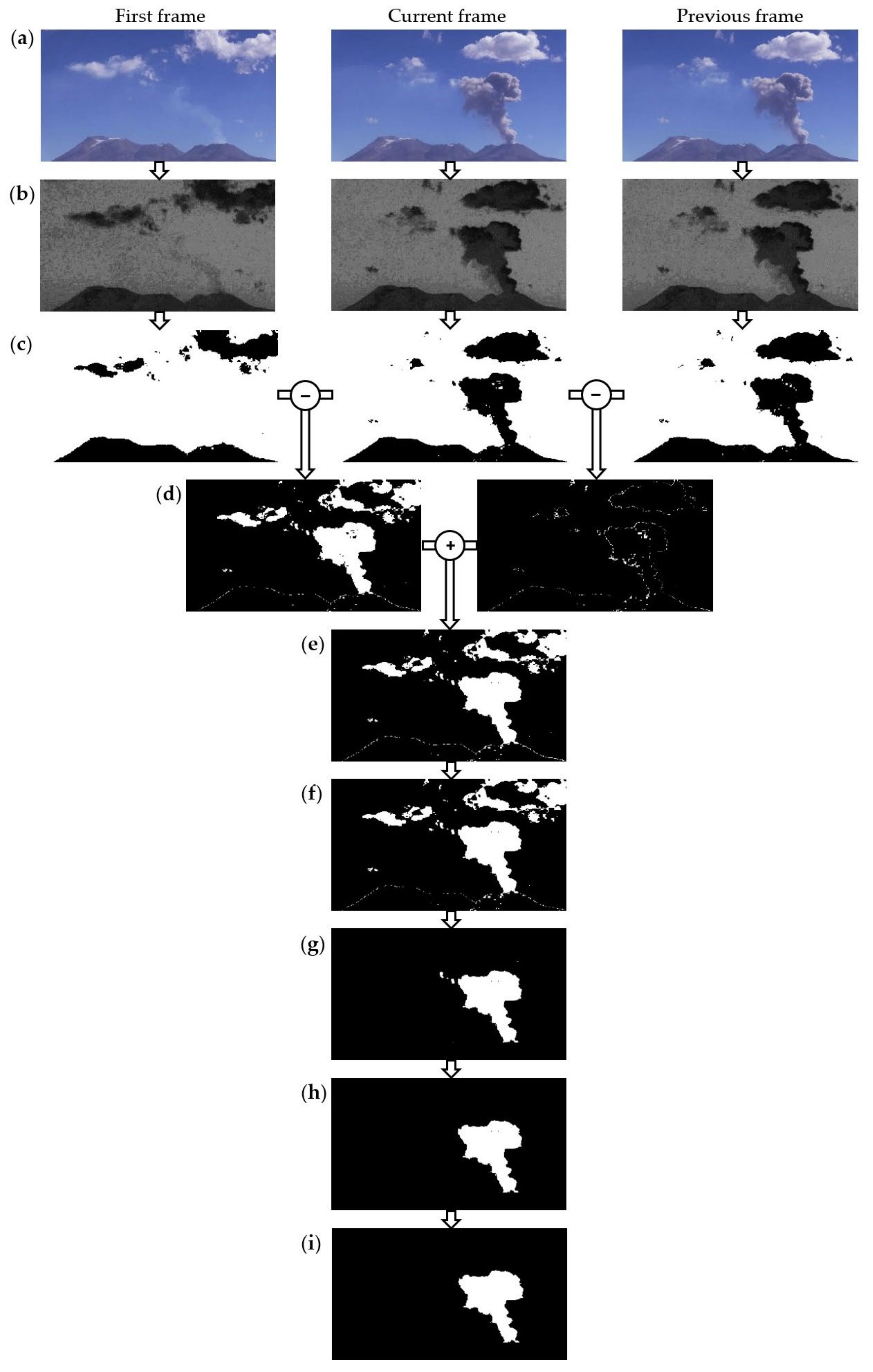
- To produce a segmented plume image for a given frame, three images are required (Figure 2a):
- the image of the current frame (at time );
- an initial image captured just prior to eruption (at time ), that is intended to be a reference for the background subtraction;
- the image of the previous frame (at time ).
- The RGB multichannel images are split into their red, green and blue channels, obtaining three images in which each pixel has a specific value of brightness intensity between 0 and 255.
- For each image, the red channel is subtracted from the blue channel as, during testing and development, we found that this commonly increases the contrast between the plume and the background compared to other possible operations. The result is an image where the plume and the landscape are highlighted with respect of the rest of the image (Figure 2b).
- A segmentation process is then applied to create binary images using a user-defined threshold pixel intensity value (Figure 2c). This threshold luminance value is determined during a pre-processing step and iterated until a satisfactory segmented output is obtained. Suggested values and additional information about the pre-processing can be found in Appendix A (Appendix A.3).
- Two partial masks are created by exploiting the difference in intensity between the images (Figure 2d):
- the first one consists of the modulus of the subtraction of the segmented first frame from the segmented current frame, resulting in a binary image that shows the plume without the landscape. However, some meteorological clouds (if they are moving) and some noise may remain. In the case of the first frame, the subtraction gives an empty image;
- the second results from the modulus of the difference between the segmented current frame and the segmented previous frame (this is not applied to the first frame, as a preceding image does not exist). Thus, it highlights the local movement of the plume (and the meteorological clouds) between frames and is fundamental to creating a mask that fits the original plume extension [15].
- The two masks are then summed (Figure 2e), which goes a long way towards enabling identification of the presence and evolution of the plume. However, it is still not fully isolated from the rest of the image.
- A two-dimensional median filter is applied, using a window of 4 × 4 pixels, to remove noise (Figure 2f).
- A mask is then applied such that all the pixels outside a region of interest (ROI) containing the plume are set equal to zero. This ROI is selected as the minimum rectangular area that captures the plume on the last frame and can be drawn automatically or manually during the pre-processing step (see Appendix A.3). This mask is essential for ensuring that the plume is selected rather than other similar objects (e.g., atmospheric clouds, degassing clouds or the landscape if its intensity and contrast are similar to those of the plume) (Figure 2g).
- All objects (white regions) apart from the largest are removed, thus removing noise and objects not connected with the plume (Figure 2h).
- Finally, holes in the remaining object are filled, leading to the final image with the extracted plume shape (Figure 2i).
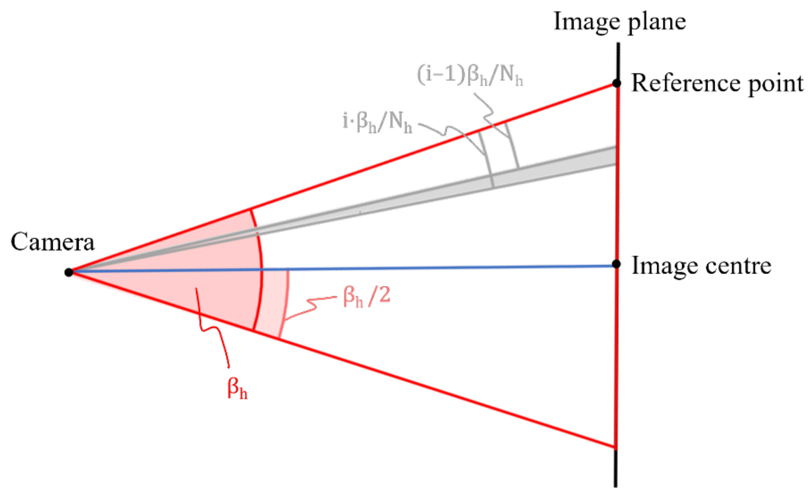
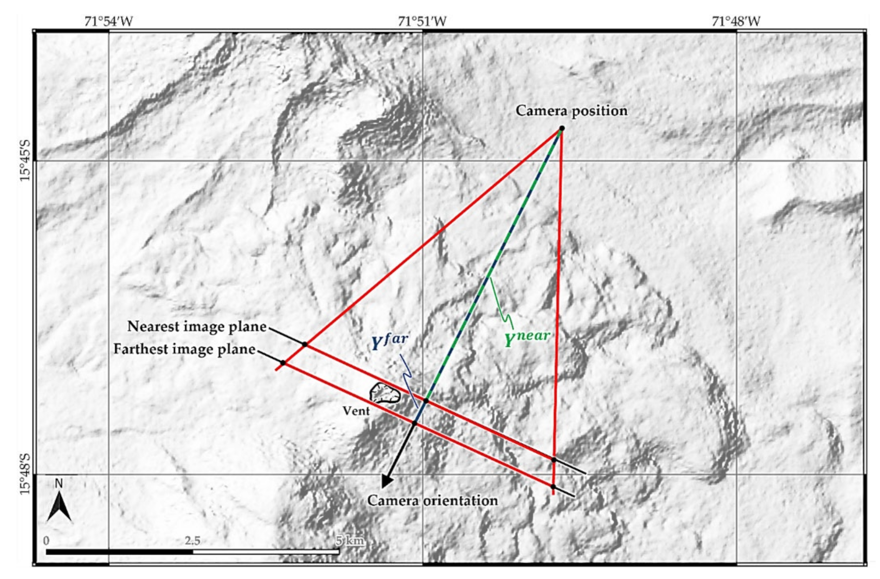
3.2. Geometrical Calibration
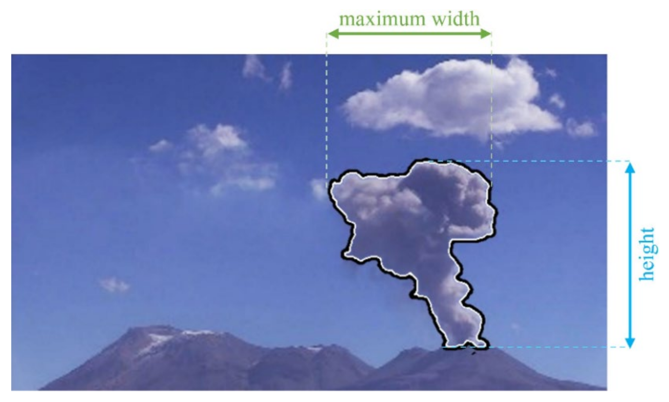
3.3. Calculation of Parameters
4. Results
4.1. Image Processing Techniques
4.2. Geometrical Calibration
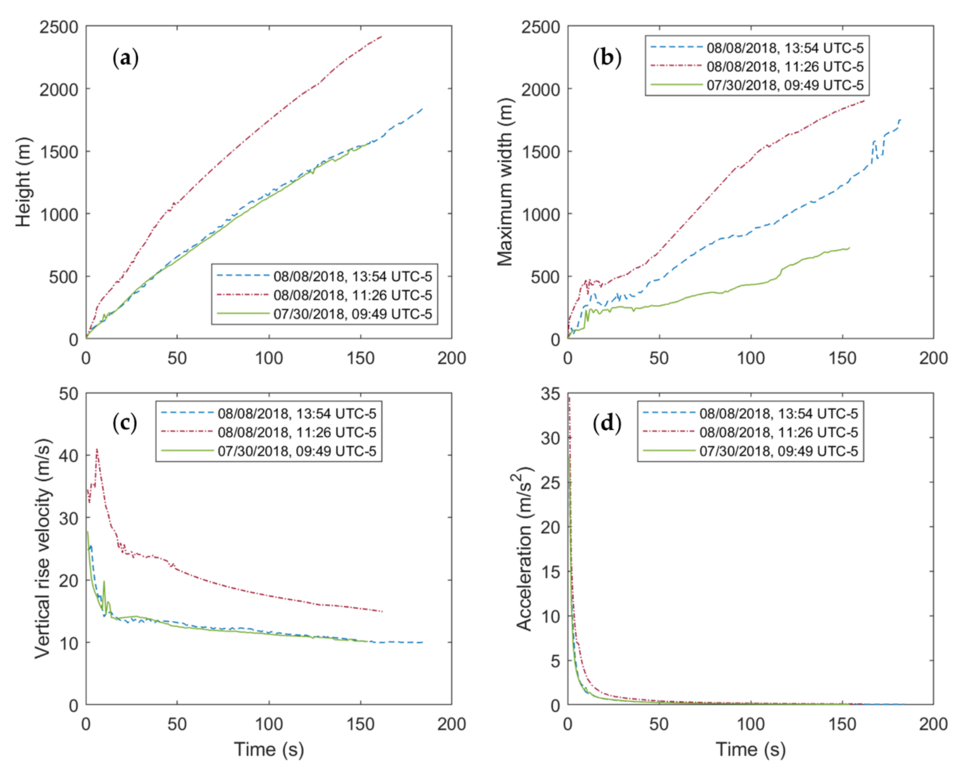
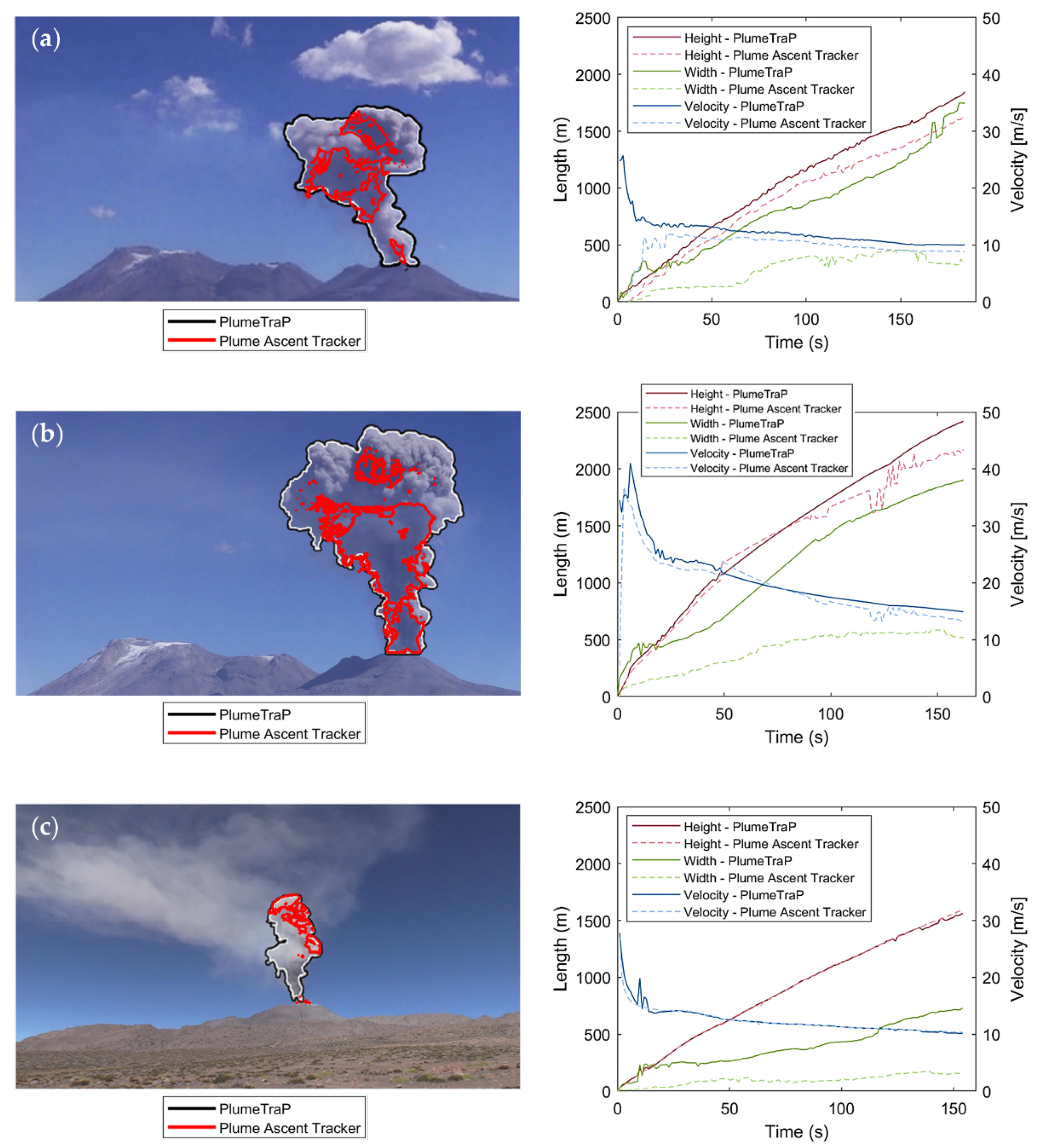
4.3. Extracted Parameters
5. Discussion
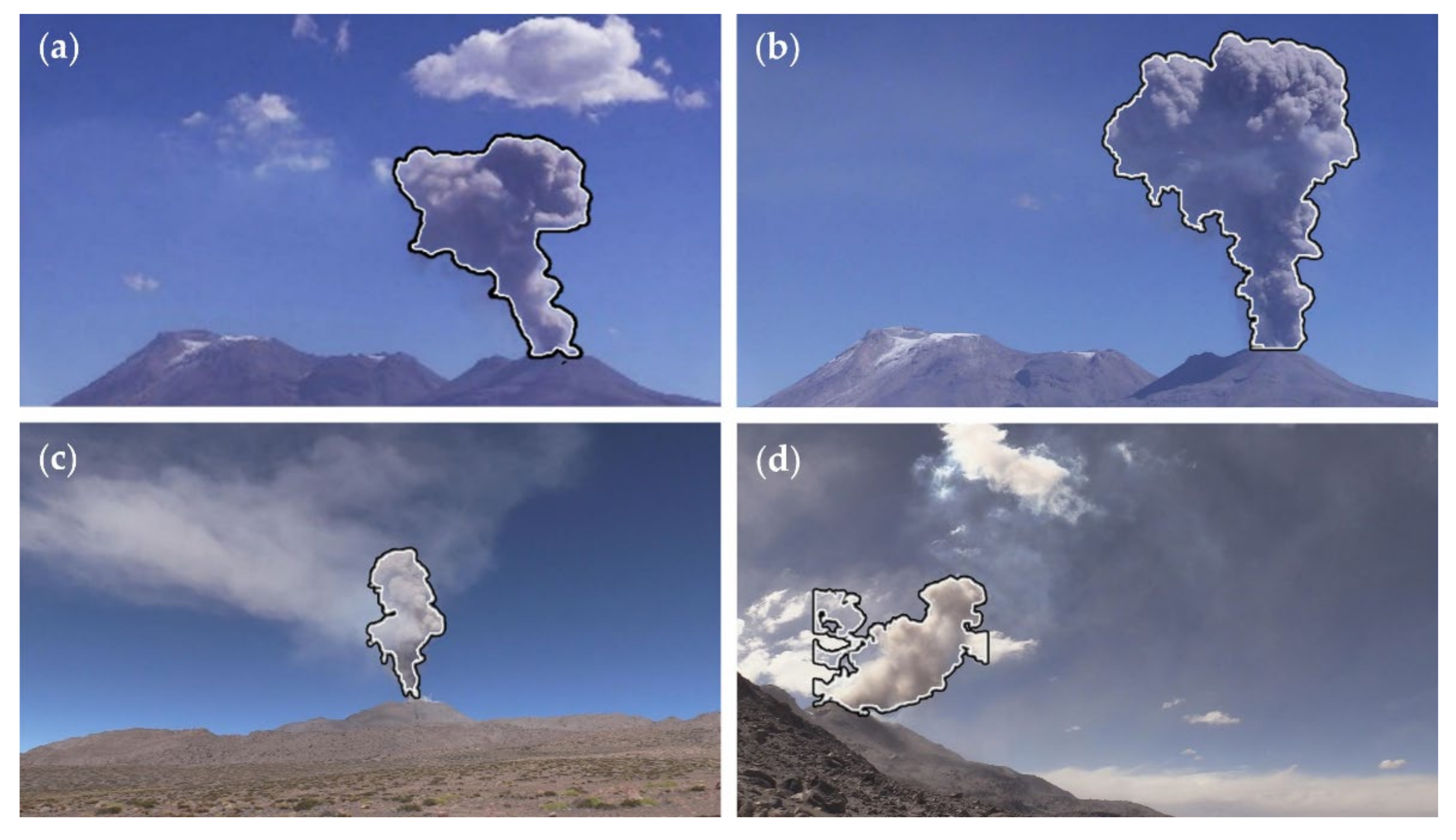
- poor contrast between the plume-shaped object and the background;
- dark light conditions and/or cloudy background;
- the presence of meteorological clouds inside the ROI;
- abundant gas emissions from the vent that form dense degassing clouds in the image background (only for the case of volcanic tephra plumes).
6. Conclusions
Supplementary Materials
Author Contributions
Funding
Institutional Review Board Statement
Informed Consent Statement
Data Availability Statement
Acknowledgments
Conflicts of Interest
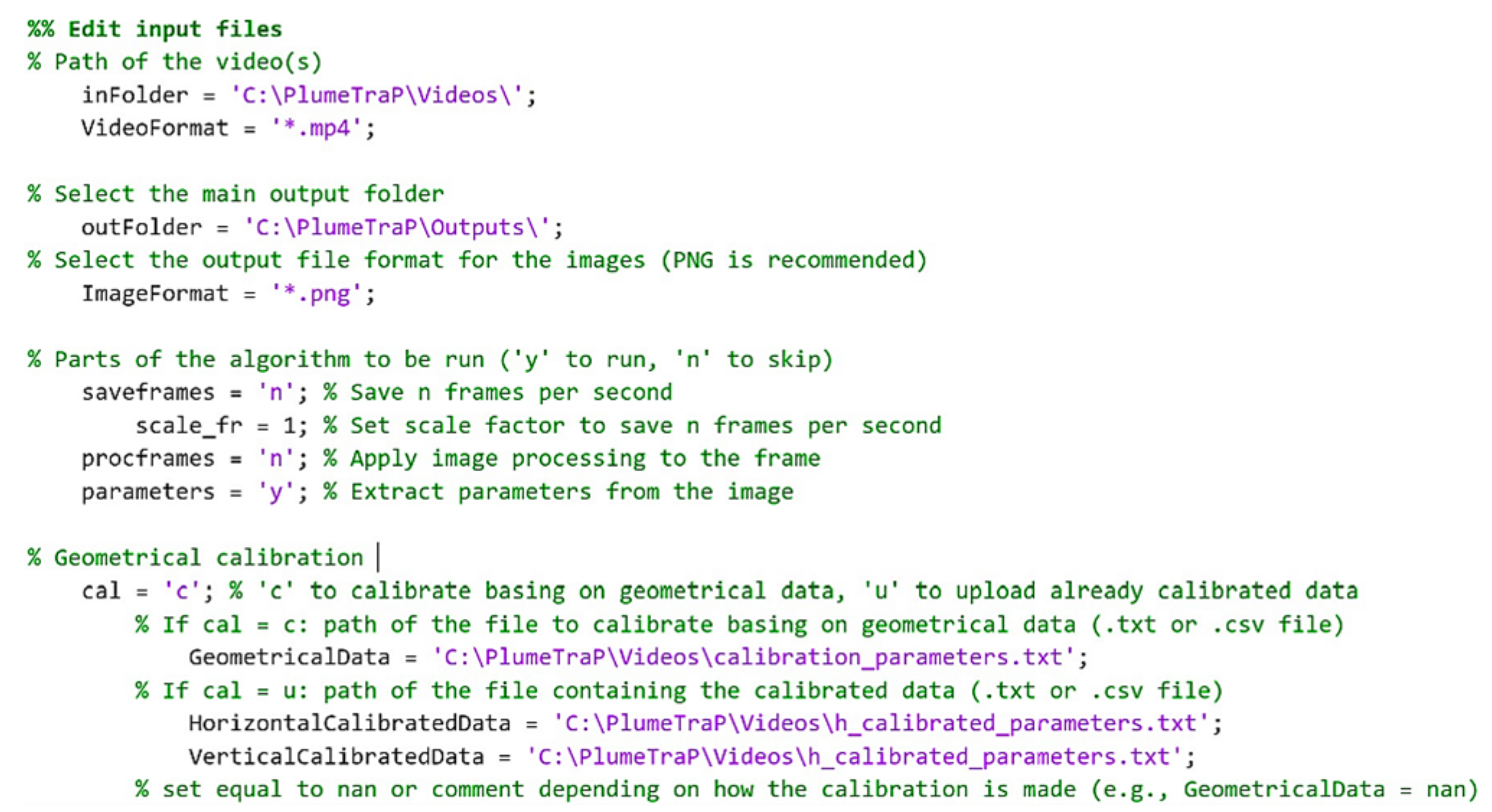
Appendix A. How to Set Up PlumeTrAP
Appendix A.1. Semi-Automatic Version


Appendix A.2. Interactive Version
Appendix A.3. General Workflow of PlumeTraP

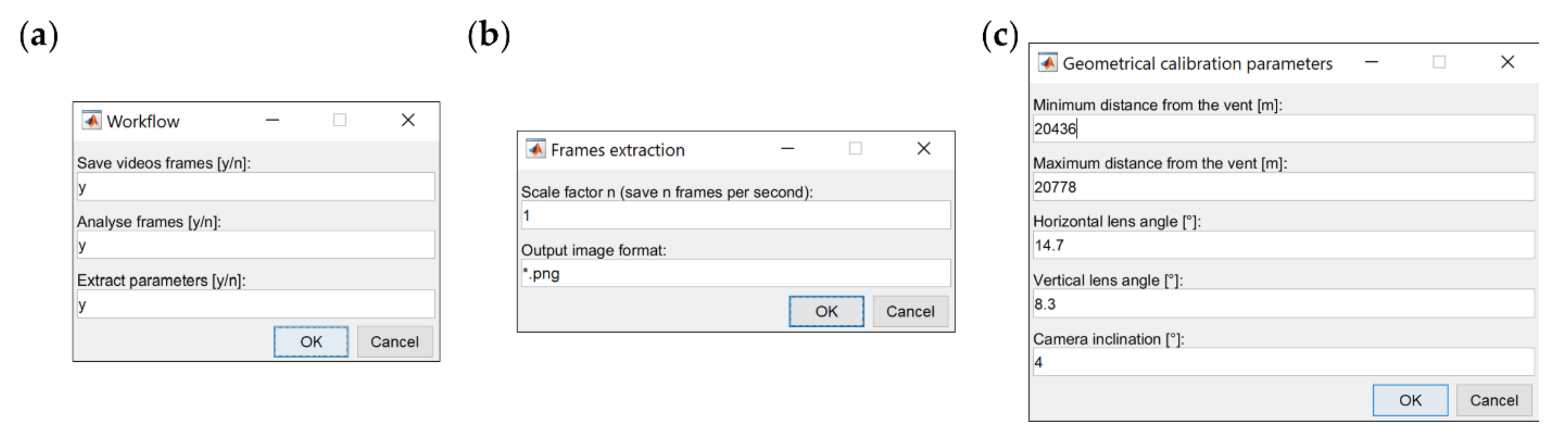
- Before starting the processing, a dialog box asks for the user to input the threshold luminance value used to create a binary image. The threshold value cannot be fixed as it reflects the luminance condition of the video and, therefore, has to be specified as a numerical scalar or numerical array with values in the range between 0 and 1, although, generally, values ranging from 0.05 to 0.2 should be used. This value can also be set using different values for the first image than for the other ones (helpful to obtain a clean background-isolated image).
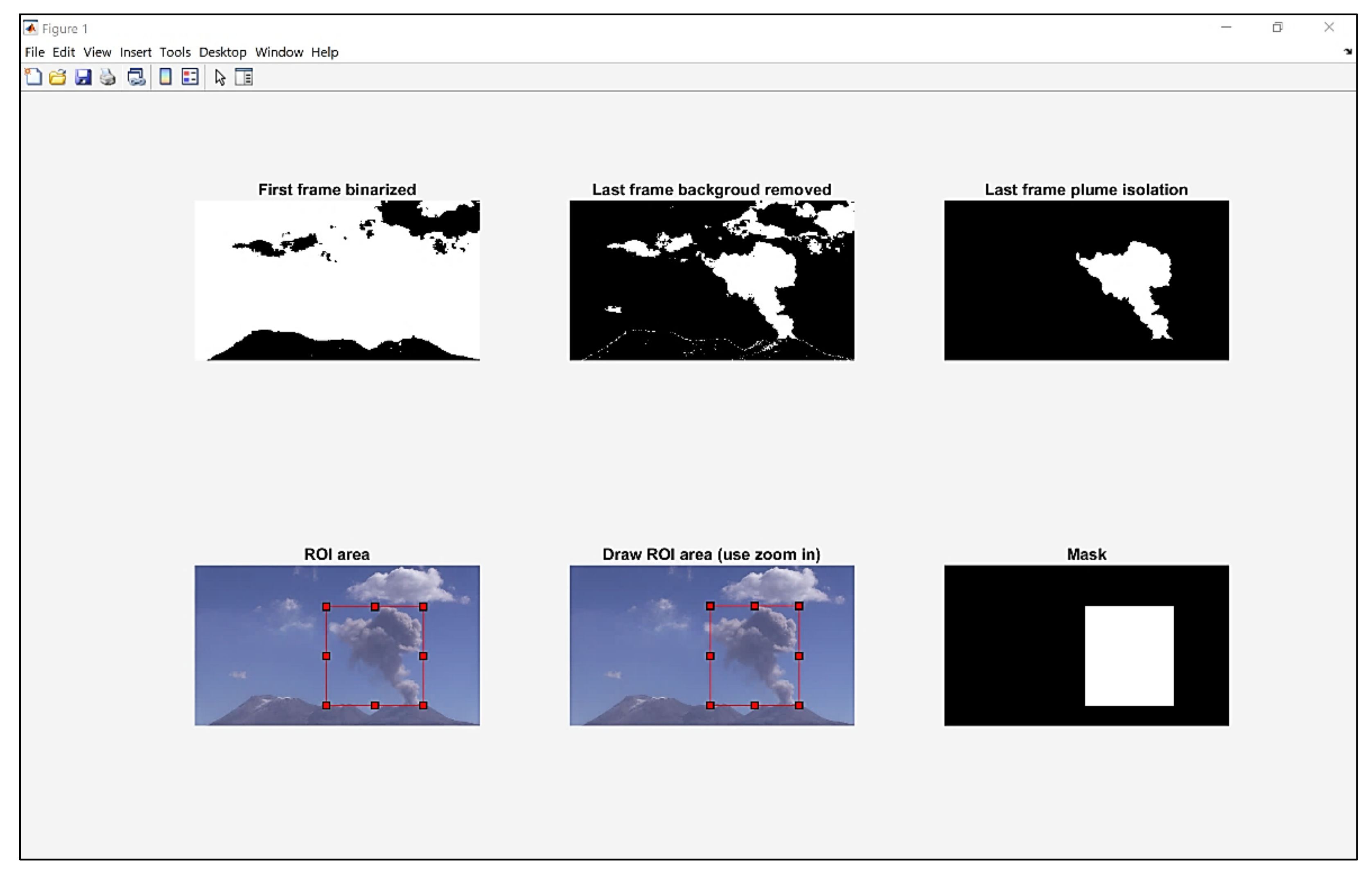
- The image analysis procedure (described in Section 3.1) is applied by the image_analysis.m function to the last frame to show a preliminary result of the analysis (Figure A5). Thus, the algorithm recognizes the plume shape in the last frame by keeping only the biggest object that has value equal to 1 in the binary image. At this point, a dialog box asks if the selected parameters isolate the plume sufficiently well. If this is not the case, it is possible to restart the pre-processing and set new thresholds, as this part of the script is inside a while loop that can be run until a satisfactory output result, mainly in terms of segmentation, is obtained.
- Once the plume seems to be well isolated from the background in the last frame, a rectangular region of interest (ROI) is drawn automatically around the plume to create a mask containing the supposed plume area. If the ROI does not correspond to or incorporate the plume well (e.g., because clouds are recognized as the bigger object), it can be drawn manually (Figure A5; zooming in is highly recommended) simply by responding to the appropriate dialog box. Then, the next dialog box asks if the user is satisfied with the drawn ROI or wants to draw it again.
Appendix B. Evaluation of Uncertainties due to Calculated Parameters
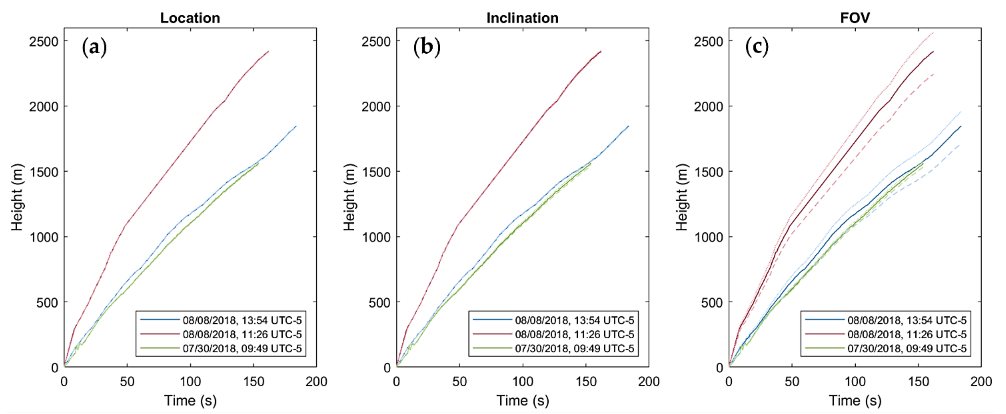
- The camera–image plane distance can be uncertain due to uncertainties in the vent and camera positions. Therefore, assuming the camera is GPS-located with a precision of ± 20 m, we find uncertainties in the plume height (Figure A7a) and maximum width (Figure A8a) to be ±0.1 % for 20 km and ± 0.3% for 5 km.
- A variation of ± 1° in the camera inclination results in a shift in the plume height (Figure A7b) of ± 0.6 % for 4° and ± 1.5% for 18°. The maximum width of the plume is not affected by this parameter.
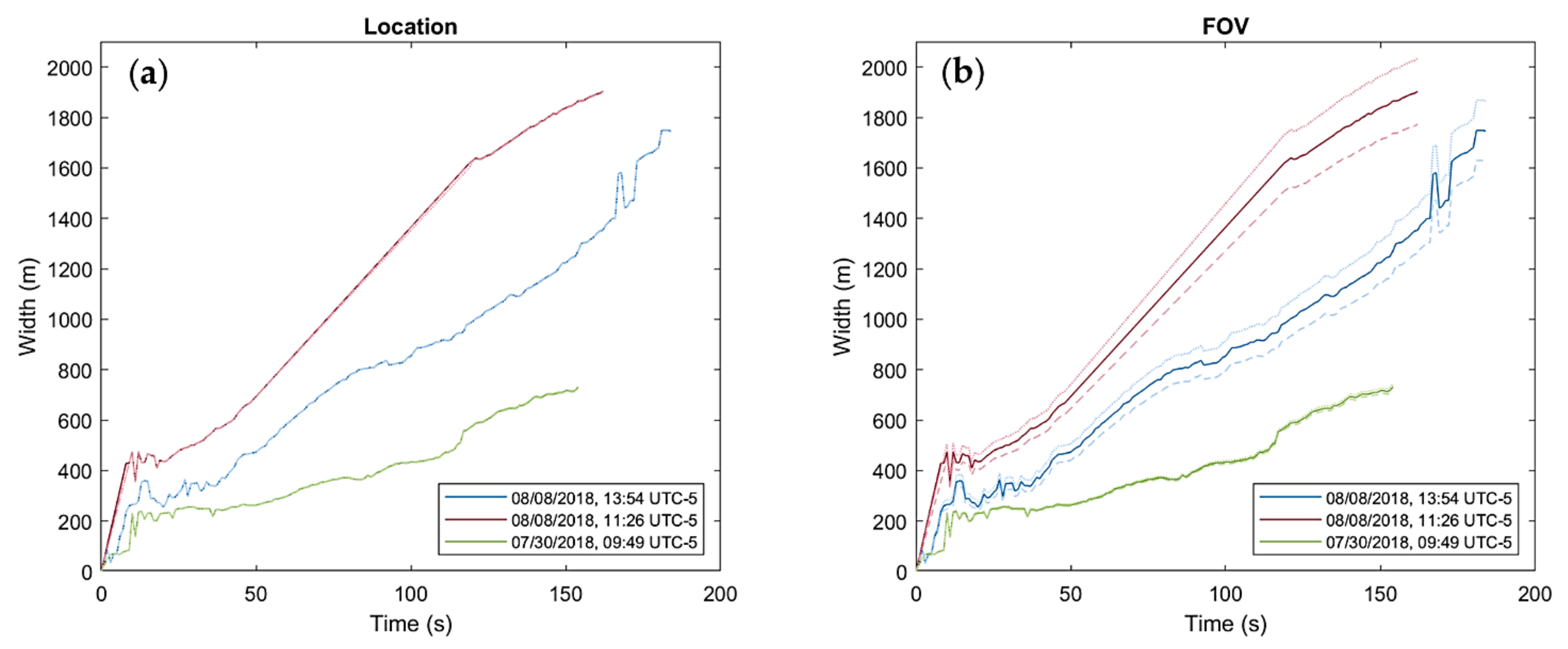
- If the FOV of the camera is unknown, the easiest way to estimate the horizontal FOV is by matching geographical locations of features in the FOV with their pixel positions. The vertical FOV can then be calculated using the image aspect ratio. We find that an error of ± 1° in the estimate of results in an error of ± (0.5–0.6)° in . This uncertainty propagates through to the calculation of the plume height (Figure A7c) and maximum width (Figure A8b) and is found to be ± 1.5% for an FOV of 69.3° × 39.0° and ± 7% for an FOV of 14.7° × 8.3°. Therefore, the FOV is the parameter that can cause the greatest error in the calculated main parameters of the plume.
References
- Sigurdsson, H.; Houghton, B.F.; McNutt, S.R.; Rymer, H.; Stix, J. (Eds.) The Encyclopedia of Volcanoes, 2nd ed.; Elsevier: Amsterdam, The Netherlands; Boston, MA, USA, 2015; ISBN 978-0-12-385938-9. [Google Scholar]
- Jenkins, S.F.; Wilson, T.M.; Magill, C.; Miller, V.; Stewart, C.; Blong, R.; Marzocchi, W.; Boulton, M.; Bonadonna, C.; Costa, A. Volcanic Ash Fall Hazard and Risk. In Global Volcanic Hazards and Risk; Vye-Brown, C., Brown, S.K., Sparks, S., Loughlin, S.C., Jenkins, S.F., Eds.; Cambridge University Press: Cambridge, UK, 2015; pp. 173–222. ISBN 978-1-107-11175-2. [Google Scholar]
- Wilson, T.M.; Cole, J.W.; Stewart, C.; Cronin, S.J.; Johnston, D.M. Ash Storms: Impacts of Wind-Remobilised Volcanic Ash on Rural Communities and Agriculture Following the 1991 Hudson Eruption, Southern Patagonia, Chile. Bull. Volcanol. 2011, 73, 223–239. [Google Scholar] [CrossRef]
- Wilson, T.M.; Stewart, C.; Sword-Daniels, V.; Leonard, G.S.; Johnston, D.M.; Cole, J.W.; Wardman, J.; Wilson, G.; Barnard, S.T. Volcanic Ash Impacts on Critical Infrastructure. Phys. Chem. Earth Parts ABC 2012, 45–46, 5–23. [Google Scholar] [CrossRef]
- Horwell, C.J.; Baxter, P.J. The Respiratory Health Hazards of Volcanic Ash: A Review for Volcanic Risk Mitigation. Bull. Volcanol. 2006, 69, 1–24. [Google Scholar] [CrossRef]
- Folch, A. A Review of Tephra Transport and Dispersal Models: Evolution, Current Status, and Future Perspectives. J. Volcanol. Geotherm. Res. 2012, 235–236, 96–115. [Google Scholar] [CrossRef]
- Connor, C.; Bebbington, M.; Marzocchi, W. Chapter 51—Probabilistic Volcanic Hazard Assessment. In The Encyclopedia of Volcanoes, 2nd ed.; Sigurdsson, H., Ed.; Academic Press: Amsterdam, The Netherlands, 2015; pp. 897–910. ISBN 978-0-12-385938-9. [Google Scholar]
- Scollo, S.; Prestifilippo, M.; Spata, G.; D’Agostino, M.; Coltelli, M. Monitoring and Forecasting Etna Volcanic Plumes. Nat. Hazards Earth Syst. Sci. 2009, 9, 1573–1585. [Google Scholar] [CrossRef] [Green Version]
- Campion, R.; Salerno, G.G.; Coheur, P.-F.; Hurtmans, D.; Clarisse, L.; Kazahaya, K.; Burton, M.; Caltabiano, T.; Clerbaux, C.; Bernard, A. Measuring Volcanic Degassing of SO2 in the Lower Troposphere with ASTER Band Ratios. J. Volcanol. Geotherm. Res. 2010, 194, 42–54. [Google Scholar] [CrossRef]
- Corradini, S.; Montopoli, M.; Guerrieri, L.; Ricci, M.; Scollo, S.; Merucci, L.; Marzano, F.; Pugnaghi, S.; Prestifilippo, M.; Ventress, L.; et al. A Multi-Sensor Approach for Volcanic Ash Cloud Retrieval and Eruption Characterization: The 23 November 2013 Etna Lava Fountain. Remote Sens. 2016, 8, 58. [Google Scholar] [CrossRef] [Green Version]
- Ripepe, M.; Marchetti, E.; Delle Donne, D.; Genco, R.; Innocenti, L.; Lacanna, G.; Valade, S. Infrasonic Early Warning System for Explosive Eruptions. J. Geophys. Res. Solid Earth 2018, 123, 9570–9585. [Google Scholar] [CrossRef]
- Scollo, S.; Prestifilippo, M.; Bonadonna, C.; Cioni, R.; Corradini, S.; Degruyter, W.; Rossi, E.; Silvestri, M.; Biale, E.; Carparelli, G.; et al. Near-Real-Time Tephra Fallout Assessment at Mt. Etna, Italy. Remote Sens. 2019, 11, 2987. [Google Scholar] [CrossRef] [Green Version]
- Cigna, F.; Tapete, D.; Lu, Z. Remote Sensing of Volcanic Processes and Risk. Remote Sens. 2020, 12, 2567. [Google Scholar] [CrossRef]
- Freret-Lorgeril, V.; Bonadonna, C.; Corradini, S.; Donnadieu, F.; Guerrieri, L.; Lacanna, G.; Marzano, F.S.; Mereu, L.; Merucci, L.; Ripepe, M.; et al. Examples of Multi-Sensor Determination of Eruptive Source Parameters of Explosive Events at Mount Etna. Remote Sens. 2021, 13, 2097. [Google Scholar] [CrossRef]
- Bombrun, M.; Jessop, D.; Harris, A.; Barra, V. An Algorithm for the Detection and Characterisation of Volcanic Plumes Using Thermal Camera Imagery. J. Volcanol. Geotherm. Res. 2018, 352, 26–37. [Google Scholar] [CrossRef]
- Patrick, M.R.; Harris, A.J.L.; Ripepe, M.; Dehn, J.; Rothery, D.A.; Calvari, S. Strombolian Explosive Styles and Source Conditions: Insights from Thermal (FLIR) Video. Bull. Volcanol. 2007, 69, 769–784. [Google Scholar] [CrossRef]
- Sahetapy-Engel, S.T.; Harris, A.J.L. Thermal-Image-Derived Dynamics of Vertical Ash Plumes at Santiaguito Volcano, Guatemala. Bull. Volcanol. 2009, 71, 827–830. [Google Scholar] [CrossRef]
- Valade, S.A.; Harris, A.J.L.; Cerminara, M. Plume Ascent Tracker: Interactive Matlab Software for Analysis of Ascending Plumes in Image Data. Comput. Geosci. 2014, 66, 132–144. [Google Scholar] [CrossRef]
- Sparks, R.S.J.; Wilson, L. Explosive Volcanic Eruptions—V. Observations of Plume Dynamics during the 1979 Soufrière Eruption, St Vincent. Geophys. J. Int. 1982, 69, 551–570. [Google Scholar] [CrossRef] [Green Version]
- Clarke, A.B.; Voight, B.; Neri, A.; Macedonio, G. Transient Dynamics of Vulcanian Explosions and Column Collapse. Nature 2002, 415, 897–901. [Google Scholar] [CrossRef]
- Formenti, Y.; Druitt, T.H.; Kelfoun, K. Characterisation of the 1997 Vulcanian Explosions of Soufrière Hills Volcano, Montserrat, by Video Analysis. Bull. Volcanol. 2003, 65, 587–605. [Google Scholar] [CrossRef]
- Tournigand, P.-Y.; Taddeucci, J.; Gaudin, D.; Fernández, J.J.P.; Bello, E.D.; Scarlato, P.; Kueppers, U.; Sesterhenn, J.; Yokoo, A. The Initial Development of Transient Volcanic Plumes as a Function of Source Conditions. J. Geophys. Res. Solid Earth 2017, 122, 9784–9803. [Google Scholar] [CrossRef]
- Contreras, R.A.; Maquerhua, E.T.; Vera, Y.A.; Gonzales, M.O.; Choquehuayta, F.A.; Mamani, L.C. Hazard Assessment Studies and Multiparametric Volcano Monitoring Developed by the Instituto Geológico, Minero y Metalúrgico in Peru. Volcanica 2021, 4, 73–92. [Google Scholar] [CrossRef]
- Kilgour, G.; Kennedy, B.; Scott, B.; Christenson, B.; Jolly, A.; Asher, C.; Rosenberg, M.; Saunders, K. Whakaari/White Island: A Review of New Zealand’s Most Active Volcano. N. Z. J. Geol. Geophys. 2021, 64, 273–295. [Google Scholar] [CrossRef]
- Spampinato, L.; Calvari, S.; Oppenheimer, C.; Boschi, E. Volcano Surveillance Using Infrared Cameras. Earth-Sci. Rev. 2011, 106, 63–91. [Google Scholar] [CrossRef]
- Rivera Porras, M.A.; Mariño Salazar, J.; Samaniego Eguiguren, P.; Delgado Ramos, R.; Manrique Llerena, N. Geología y evaluación de peligros del complejo volcánico Ampato-Sabancaya, Arequipa-[Boletín C 61]. Inst. Geológico Min. Met. INGEMMET 2016. Available online: https://hdl.handle.net/20.500.12544/297 (accessed on 26 June 2021).
- Mariño Salazar, J.; Rivera Porras, M.A.; Samaniego Eguiguren, P.; Macedo Franco, L.D. Evaluación y zonificación de peligros volcán Sabancaya, región Arequipa. Inst. Geológico Min. Met. INGEMMET 2016. Available online: https://hdl.handle.net/20.500.12544/993 (accessed on 26 June 2021).
- Gerbe, M.-C.; Thouret, J.-C. Role of Magma Mixing in the Petrogenesis of Tephra Erupted during the 1990–98 Explosive Activity of Nevado Sabancaya, Southern Peru. Bull. Volcanol. 2004, 66, 541–561. [Google Scholar] [CrossRef]
- MacQueen, P.; Delgado, F.; Reath, K.; Pritchard, M.E.; Bagnardi, M.; Milillo, P.; Lundgren, P.; Macedo, O.; Aguilar, V.; Ortega, M.; et al. Volcano-Tectonic Interactions at Sabancaya Volcano, Peru: Eruptions, Magmatic Inflation, Moderate Earthquakes, and Fault Creep. J. Geophys. Res. Solid Earth 2020, 125, e2019JB019281. [Google Scholar] [CrossRef]
- Global Volcanism Program, 2018. Report on Sabancaya (Peru). Sennert, S.K., (Ed.); Weekly Volcanic Activity Report. 1–7 August 2018. Smithsonian Institution and US Geological Survey. Available online: https://volcano.si.edu/ShowReport.cfm?doi=10.5479/si.GVP.WVAR20180801-354006 (accessed on 26 June 2021).
- Global Volcanism Program, 2018. Report on Sabancaya (Peru). Sennert, S.K., (Ed.); Weekly Volcanic Activity Report. 8–14 August 2018. Smithsonian Institution and US Geological Survey. Available online: https://volcano.si.edu/ShowReport.cfm?doi=10.5479/si.GVP.WVAR20180808-354006 (accessed on 26 June 2021).
- Global Volcanism Program, 2018. Report on Sabancaya (Peru). Sennert, S.K. (Ed.); Weekly Volcanic Activity Report. 25–31 July 2018. Smithsonian Institution and US Geological Survey. Available online: https://volcano.si.edu/ShowReport.cfm?doi=10.5479/si.GVP.WVAR20180725-354006 (accessed on 26 June 2021).
- Schneider, C.A.; Rasband, W.S.; Eliceiri, K.W. NIH Image to ImageJ: 25 Years of Image Analysis. Nat. Methods 2012, 9, 671–675. [Google Scholar] [CrossRef]
- Sommer, C.; Straehle, C.; Köthe, U.; Hamprecht, F.A. Ilastik: Interactive Learning and Segmentation Toolkit. In Proceedings of the 2011 IEEE International Symposium on Biomedical Imaging: From Nano to Macro, Chicago, IL, USA, 30 March–2 April 2011; pp. 230–233. [Google Scholar]
- Snee, E.; Jarvis, P.A.; Simionato, R.; Scollo, S.; Prestifilippo, M.; Degruyter, W.; Bonadonna, C. Image Analysis of Volcanic Plumes: A Simple Calibration Tool to Correct for the Effect of Wind. Volcanica, 2022; submitted. [Google Scholar]
- Woods, A.W.; Kienle, J. The Dynamics and Thermodynamics of Volcanic Clouds: Theory and Observations from the 15 April and 21 April 1990 Eruptions of Redoubt Volcano, Alaska. J. Volcanol. Geotherm. Res. 1994, 62, 273–299. [Google Scholar] [CrossRef]
- Yamamoto, H.; Watson, I.M.; Phillips, J.C.; Bluth, G.J. Rise Dynamics and Relative Ash Distribution in Vulcanian Eruption Plumes at Santiaguito Volcano, Guatemala, Revealed Using an Ultraviolet Imaging Camera. Geophys. Res. Lett. 2008, 35, L08314. [Google Scholar] [CrossRef]
- Bonadonna, C.; Macedonio, G.; Sparks, R.S.J. Numerical Modelling of Tephra Fallout Associated with Dome Collapses and Vulcanian Explosions: Application to Hazard Assessment on Montserrat. Geol. Soc. Lond. Mem. 2002, 21, 517–537. [Google Scholar] [CrossRef] [Green Version]
- Supported Video and Audio File Formats-MATLAB & Simulink-MathWorks United Kingdom. Available online: https://uk.mathworks.com/help/matlab/import_export/supported-video-file-formats.html (accessed on 20 October 2021).


| No. of Frames | Computer A 1 | Computer B 2 | |
|---|---|---|---|
| Read video | 185 | 2.482 s | 69.331 s |
| 20 | 1.325 s | 8.885 s | |
| Save video frames | 185 | 0.614 fps | 1.445 fps |
| 20 | 0.473 fps | 1.458 fps | |
| Frame processing | 185 | 0.532 fps | 1.557 fps |
| 20 | 0.347 fps | 1.481 fps | |
| Geometric calibration | 185 | 0.254 s | 0.042 s |
| 20 | 0.223 s | 0.057 s | |
| Calculation of parameters | 185 | 0.573 fps | 1.340 fps |
| 20 | 0.641 fps | 2.311 fps | |
| Total (frame-dependent) | 185 | 0.190 fps | 0.481 fps |
| 20 | 0.153 fps | 0.558 fps |
Publisher’s Note: MDPI stays neutral with regard to jurisdictional claims in published maps and institutional affiliations. |
© 2022 by the authors. Licensee MDPI, Basel, Switzerland. This article is an open access article distributed under the terms and conditions of the Creative Commons Attribution (CC BY) license (https://creativecommons.org/licenses/by/4.0/).
Share and Cite
Simionato, R.; Jarvis, P.A.; Rossi, E.; Bonadonna, C. PlumeTraP: A New MATLAB-Based Algorithm to Detect and Parametrize Volcanic Plumes from Visible-Wavelength Images. Remote Sens. 2022, 14, 1766. https://doi.org/10.3390/rs14071766
Simionato R, Jarvis PA, Rossi E, Bonadonna C. PlumeTraP: A New MATLAB-Based Algorithm to Detect and Parametrize Volcanic Plumes from Visible-Wavelength Images. Remote Sensing. 2022; 14(7):1766. https://doi.org/10.3390/rs14071766
Chicago/Turabian StyleSimionato, Riccardo, Paul A. Jarvis, Eduardo Rossi, and Costanza Bonadonna. 2022. "PlumeTraP: A New MATLAB-Based Algorithm to Detect and Parametrize Volcanic Plumes from Visible-Wavelength Images" Remote Sensing 14, no. 7: 1766. https://doi.org/10.3390/rs14071766
APA StyleSimionato, R., Jarvis, P. A., Rossi, E., & Bonadonna, C. (2022). PlumeTraP: A New MATLAB-Based Algorithm to Detect and Parametrize Volcanic Plumes from Visible-Wavelength Images. Remote Sensing, 14(7), 1766. https://doi.org/10.3390/rs14071766