
InSAR Study of Landslides: Early Detection, Three-Dimensional, and Long-Term Surface Displacement Estimation—A Case of Xiaojiang River Basin, China


Abstract
:1. Introduction
2. Study area and Datasets
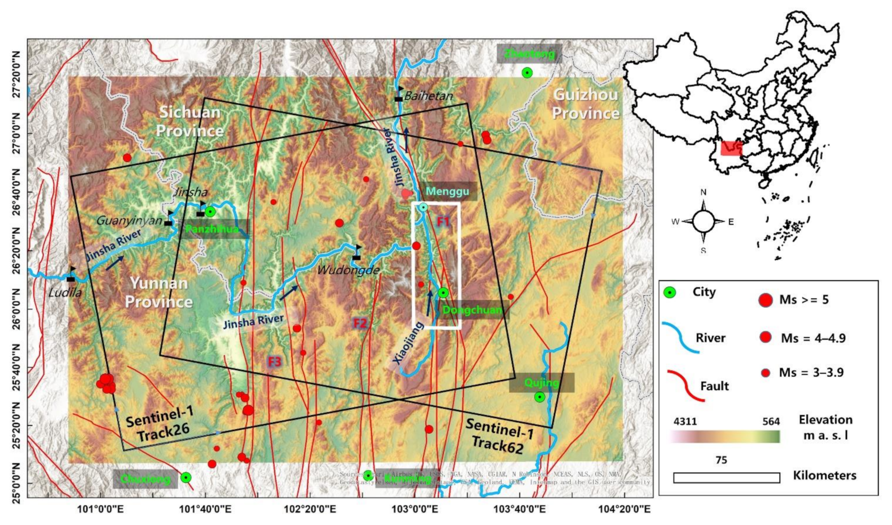
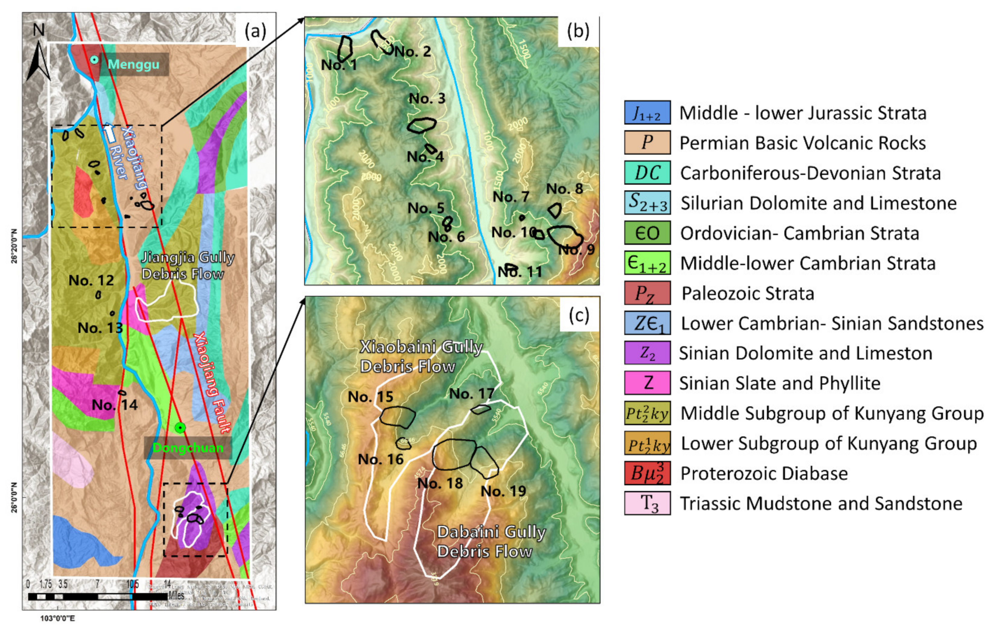
2.1. Study Area
2.2. Datasets
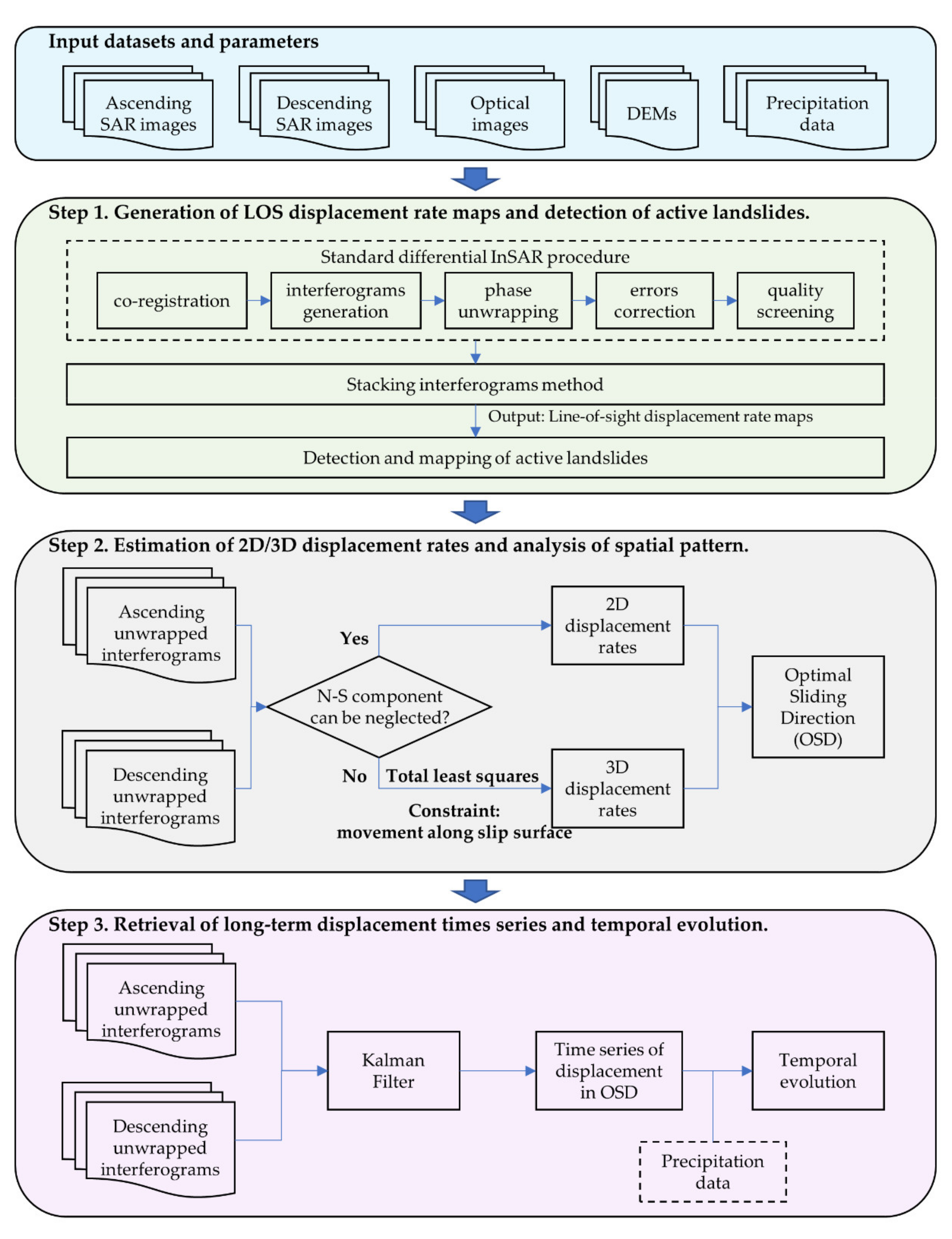
3. Methodology
3.1. InSAR Processing
3.2. Total Least Squares Estimation of Three-Dimensional Landslide Displacement Rates
3.3. Kalman Filter for Long-Term Landslide Displacement Time Series
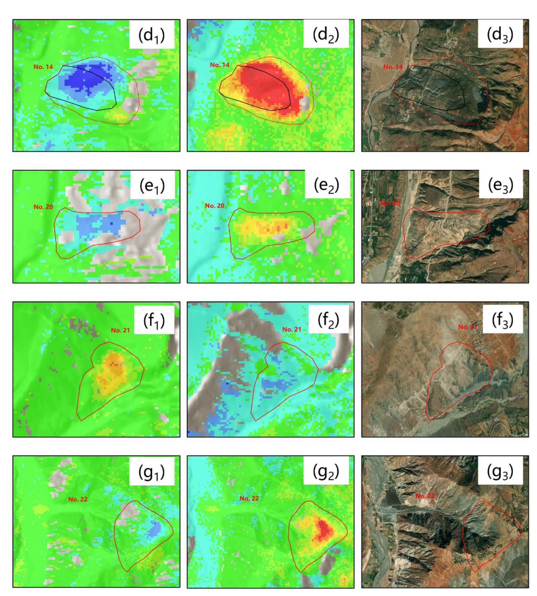
4. Results: Line-of-Sight Displacement Rates between March 2007 to May 2019
5. Discussion: Three-Dimensional and Long-Term Displacements of Baobao Landslide
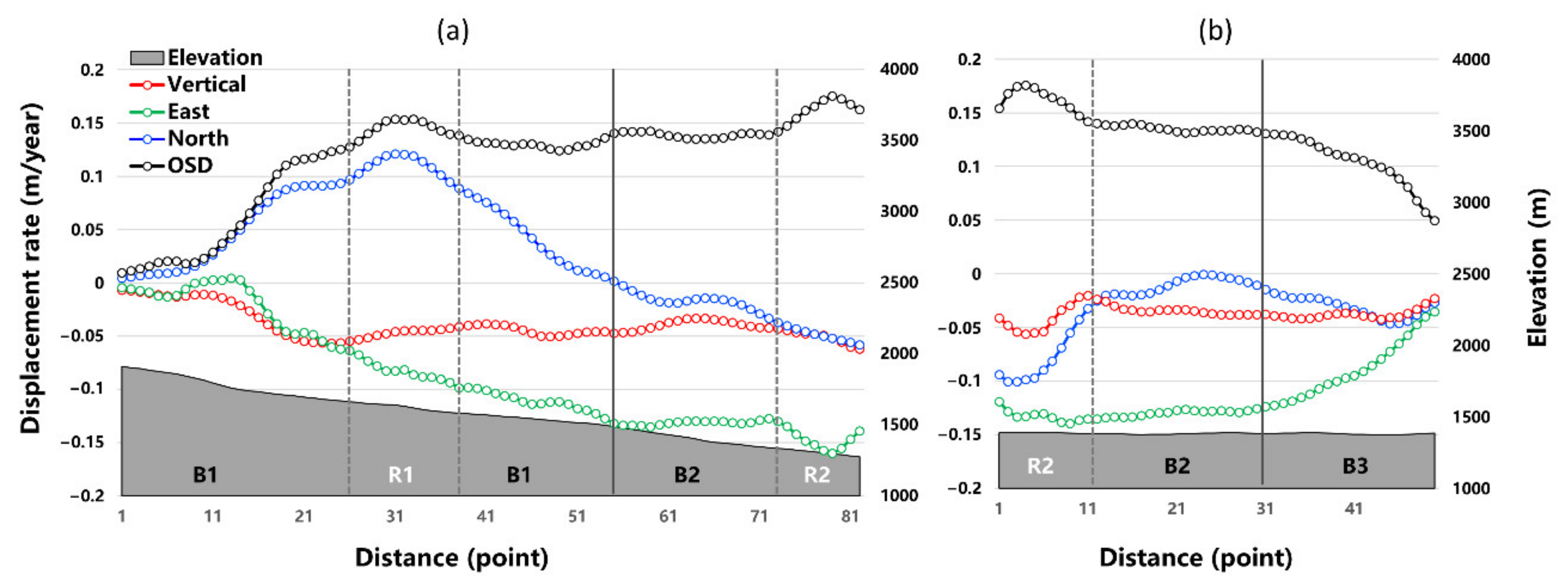
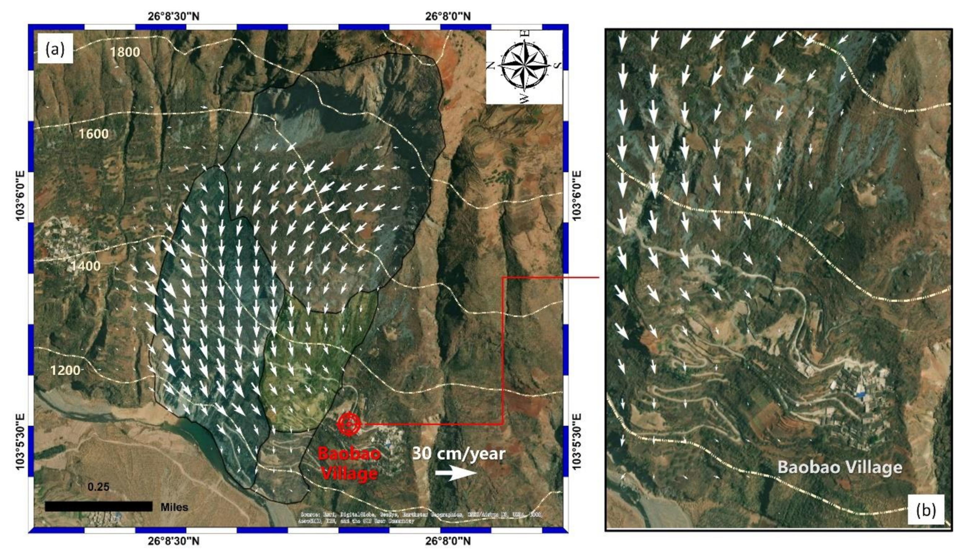
5.1. Three-Dimensional Displacement Rates for Spatial Displacement Pattern Analysis
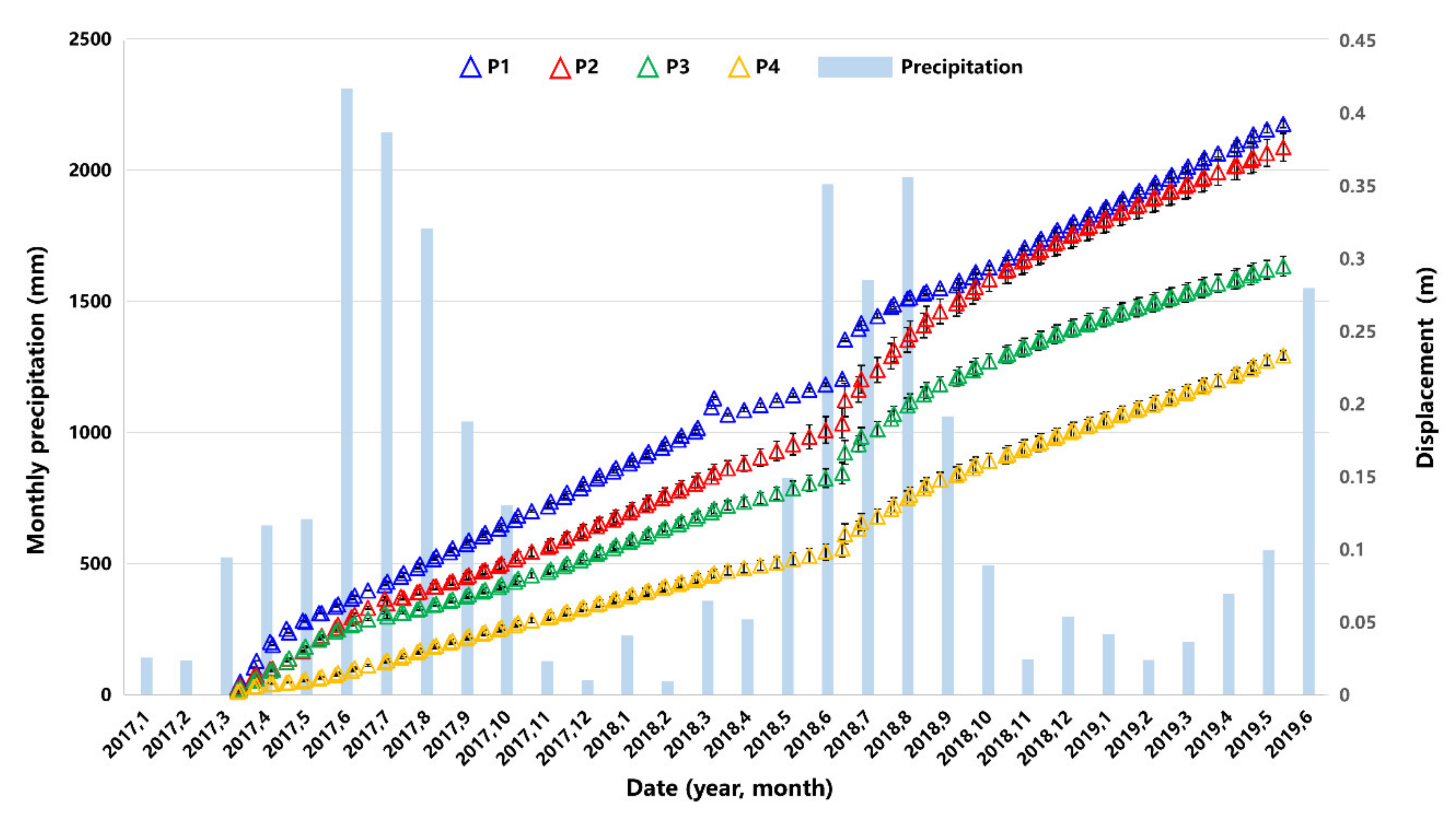
5.2. Long-Term Displacement Time Series for Temporal Displacement Pattern Analysis
6. Conclusions
Author Contributions
Funding
Institutional Review Board Statement
Informed Consent Statement
Data Availability Statement
Acknowledgments
Conflicts of Interest
References
- Necula, N.; Niculiță, M.; Fiaschi, S.; Genevois, R.; Riccardi, P.; Floris, M. Assessing Urban Landslide Dynamics through Multi-Temporal InSAR Techniques and Slope Numerical Modeling. Remote Sens. 2021, 13, 3862. [Google Scholar] [CrossRef]
- Zhu, Y.; Qiu, H.; Liu, Z.; Wang, J.; Yang, D.; Pei, Y.; Ma, S.; Du, C.; Sun, H.; Wang, L. Detecting Long-Term Deformation of a Loess Landslide from the Phase and Amplitude of Satellite SAR Images: A Retrospective Analysis for the Closure of a Tunnel Event. Remote Sens. 2021, 13, 4841. [Google Scholar] [CrossRef]
- Yang, D.; Qiu, H.; Zhu, Y.; Liu, Z.; Pei, Y.; Ma, S.; Du, C.; Sun, H.; Liu, Y.; Cao, M. Landslide Characteristics and Evolution: What We Can Learn from Three Adjacent Landslides. Remote Sens. 2021, 13, 4579. [Google Scholar] [CrossRef]
- Petley, D. Global patterns of loss of life from landslides. Geology 2012, 40, 927–930. [Google Scholar] [CrossRef]
- Froude, M.; Petley, D. Global fatal landslide occurrence from 2004 to 2016. Nat. Hazards Earth Syst. Sci. 2018, 18, 2161–2181. [Google Scholar] [CrossRef] [Green Version]
- Jia, H.; Wang, Y.; Ge, D.; Deng, Y.; Wang, R. Improved Offset Tracking for Predisaster Deformation Monitoring of the 2018 Jinsha River Landslide (Tibet, China). Remote Sens. Environ. 2020, 247, 111899. [Google Scholar] [CrossRef]
- Intrieri, E.; Raspini, F.; Fumagalli, A.; Lu, P.; del Conte, S.; Farina, P.; Allievi, J.; Ferretti, A.; Casagli, N. The Maoxian Landslide as Seen from Space: Detecting Precursors of Failure with Sentinel-1 Data. Landslides 2018, 15, 123–133. [Google Scholar] [CrossRef] [Green Version]
- Dai, K.; Li, Z.; Xu, Q.; Burgmann, R.; Milledge, D.G.; Tomas, R.; Fan, X.; Zhao, C.; Liu, X.; Peng, J.; et al. Entering the Era of Earth Observation-Based Landslide Warning Systems: A Novel and Exciting Framework. IEEE Geosci. Remote Sens. Mag. 2020, 8, 136–153. [Google Scholar] [CrossRef] [Green Version]
- Massonnet, D.; Feigl, K.L. Radar Interferometry and Its Application to Changes in the Earth’s Surface. Rev. Geophys. 1998, 36, 441–500. [Google Scholar] [CrossRef] [Green Version]
- Berardino, P.; Fornaro, G.; Lanari, R.; Sansosti, E. A New Algorithm for Surface Deformation Monitoring Based on Small Baseline Differential SAR Interferograms. IEEE Trans. Geosci. Remote Sens. 2002, 40, 2375–2383. [Google Scholar] [CrossRef] [Green Version]
- Ferretti, A.; Prati, C.; Rocca, F. Permanent Scatterers in SAR Interferometry. IEEE Trans. Geosci. Remote Sens. 2001, 39, 8–20. [Google Scholar] [CrossRef]
- Lyons, S.; Sandwell, D. Fault Creep along the Southern San Andreas from Interferometric Synthetic Aperture Radar, Permanent Scatterers, and Stacking: Southern San Andreas from Insar. J. Geophys. Res. 2003, 108, 108. [Google Scholar] [CrossRef]
- Rosi, A.; Tofani, V.; Tanteri, L.; Tacconi Stefanelli, C.; Agostini, A.; Catani, F.; Casagli, N. The New Landslide Inventory of Tuscany (Italy) Updated with PS-InSAR: Geomorphological Features and Landslide Distribution. Landslides 2018, 15, 5–19. [Google Scholar] [CrossRef] [Green Version]
- Solari, L.; del Soldato, M.; Raspini, F.; Barra, A.; Bianchini, S.; Confuorto, P.; Casagli, N.; Crosetto, M. Review of Satellite Interferometry for Landslide Detection in Italy. Remote Sens. 2020, 12, 1351. [Google Scholar] [CrossRef]
- Schlögel, R.; Doubre, C.; Malet, J.-P.; Masson, F. Landslide Deformation Monitoring with ALOS/PALSAR Imagery: A D-InSAR Geomorphological Interpretation Method. Geomorphology 2015, 231, 314–330. [Google Scholar] [CrossRef]
- Aslan, G.; Foumelis, M.; Raucoules, D.; de Michele, M.; Bernardie, S.; Cakir, Z. Landslide Mapping and Monitoring Using Persistent Scatterer Interferometry (PSI) Technique in the French Alps. Remote Sens. 2020, 12, 1305. [Google Scholar] [CrossRef] [Green Version]
- Zhao, C.; Lu, Z.; Zhang, Q.; de la Fuente, J. Large-Area Landslide Detection and Monitoring with ALOS/PALSAR Imagery Data over Northern California and Southern Oregon, USA. Remote Sens. Environ. 2012, 124, 348–359. [Google Scholar] [CrossRef]
- Zhao, C.; Kang, Y.; Zhang, Q.; Lu, Z.; Li, B. Landslide Identification and Monitoring along the Jinsha River Catchment (Wudongde Reservoir Area), China, Using the InSAR Method. Remote Sens. 2018, 10, 993. [Google Scholar] [CrossRef] [Green Version]
- Liu, X.; Zhao, C.; Zhang, Q.; Lu, Z.; Li, Z.; Yang, C.; Zhu, W.; Liu-Zeng, J.; Chen, L.; Liu, C. Integration of Sentinel-1 and ALOS/PALSAR-2 SAR Datasets for Mapping Active Landslides along the Jinsha River Corridor, China. Eng. Geol. 2021, 284, 106033. [Google Scholar] [CrossRef]
- Novellino, A.; Cigna, F.; Sowter, A.; Ramondini, M.; Calcaterra, D. Exploitation of the Intermittent SBAS (ISBAS) Algorithm with COSMO-SkyMed Data for Landslide Inventory Mapping in North-Western Sicily, Italy. Geomorphology 2017, 280, 153–166. [Google Scholar] [CrossRef]
- Bouali, E.H.; Oommen, T.; Escobar-Wolf, R. Mapping of Slow Landslides on the Palos Verdes Peninsula Using the California Landslide Inventory and Persistent Scatterer Interferometry. Landslides 2018, 15, 439–452. [Google Scholar] [CrossRef]
- Zhang, L.; Dai, K.; Deng, J.; Ge, D.; Liang, R.; Li, W.; Xu, Q. Identifying Potential Landslides by Stacking-InSAR in Southwestern China and Its Performance Comparison with SBAS-InSAR. Remote Sens. 2021, 13, 3662. [Google Scholar] [CrossRef]
- Colesanti, C.; Wasowski, J. Investigating Landslides with Space-Borne Synthetic Aperture Radar (SAR) Interferometry. Eng. Geol. 2006, 88, 173–199. [Google Scholar] [CrossRef]
- Gray, L. Using Multiple RADARSAT InSAR Pairs to Estimate a Full Three-Dimensional Solution for Glacial Ice Movement: Multiple Interferograms for 3-D Motion. Geophys. Res. Lett. 2011, 38, 38. [Google Scholar] [CrossRef]
- Wright, T.J. Toward Mapping Surface Deformation in Three Dimensions Using InSAR. Geophys. Res. Lett. 2004, 31, L01607. [Google Scholar] [CrossRef] [Green Version]
- Fialko, Y.; Sandwell, D.; Simons, M.; Rosen, P. Three-Dimensional Deformation Caused by the Bam, Iran, Earthquake and the Origin of Shallow Slip Deficit. Nature 2005, 435, 295–299. [Google Scholar] [CrossRef]
- Hu, J.; Li, Z.; Zhu, J.; Ren, X.; Ding, X. Inferring Three-Dimensional Surface Displacement Field by Combining SAR Interferometric Phase and Amplitude Information of Ascending and Descending Orbits. Sci. China Earth Sci. 2010, 53, 550–560. [Google Scholar] [CrossRef]
- Jung, H.S.; Lu, Z.; Won, J.S.; Poland, M.P.; Miklius, A. Mapping Three-Dimensional Surface Deformation by Combining Multiple-Aperture Interferometry and Conventional Interferometry: Application to the June 2007 Eruption of Kilauea Volcano, Hawaii. IEEE Geosci. Remote Sensing Lett. 2011, 8, 34–38. [Google Scholar] [CrossRef]
- Hu, J.; Li, Z.W.; Ding, X.L.; Zhu, J.J.; Zhang, L.; Sun, Q. 3D Coseismic Displacement of 2010 Darfield, New Zealand Earthquake Estimated from Multi-Aperture InSAR and D-InSAR Measurements. J. Geod. 2012, 86, 1029–1041. [Google Scholar] [CrossRef]
- Gudmundsson, S.; Sigmundsson, F.; Carstensen, J.M. Three-Dimensional Surface Motion Maps Estimated from Combined Interferometric Synthetic Aperture Radar and GPS Data: THREE-DIMENSIONAL SURFACE MOTION MAPS. J. Geophys. Res. 2002, 107, ETG 13-1–ETG 13-14. [Google Scholar] [CrossRef]
- Ji, P.; Lv, X.; Chen, Q.; Sun, G.; Yao, J. Applying InSAR and GNSS Data to Obtain 3-D Surface Deformations Based on Iterated Almost Unbiased Estimation and Laplacian Smoothness Constraint. IEEE J. Sel. Top. Appl. Earth Obs. Remote Sens. 2021, 14, 337–349. [Google Scholar] [CrossRef]
- Ji, P.; Lv, X.; Yao, J.; Sun, G. A New Method to Obtain 3-D Surface Deformations from InSAR and GNSS Data With Genetic Algorithm and Support Vector Machine. IEEE Geosci. Remote Sens. Lett. 2022, 19, 1–5. [Google Scholar] [CrossRef]
- Dong, L.; Wang, C.; Tang, Y.; Tang, F.; Zhang, H.; Wang, J.; Duan, W. Time Series InSAR Three-Dimensional Displacement Inversion Model of Coal Mining Areas Based on Symmetrical Features of Mining Subsidence. Remote Sens. 2021, 13, 2143. [Google Scholar] [CrossRef]
- Yang, Z.; Li, Z.; Zhu, J.; Feng, G.; Wang, Q.; Hu, J.; Wang, C. Deriving Time-Series Three-Dimensional Displacements of Mining Areas from a Single-Geometry InSAR Dataset. J. Geod. 2018, 92, 529–544. [Google Scholar] [CrossRef]
- Li, Z.W.; Yang, Z.F.; Zhu, J.J.; Hu, J.; Wang, Y.J.; Li, P.X.; Chen, G.L. Retrieving Three-Dimensional Displacement Fields of Mining Areas from a Single InSAR Pair. J. Geod. 2015, 89, 17–32. [Google Scholar] [CrossRef]
- Kumar, V.; Venkataramana, G.; Høgda, K.A. Glacier Surface Velocity Estimation Using SAR Interferometry Technique Applying Ascending and Descending Passes in Himalayas. Int. J. Appl. Earth Obs. Geoinf. 2011, 13, 545–551. [Google Scholar] [CrossRef]
- Sun, Q.; Hu, J.; Zhang, L.; Ding, X. Towards Slow-Moving Landslide Monitoring by Integrating Multi-Sensor InSAR Time Series Datasets: The Zhouqu Case Study, China. Remote Sens. 2016, 8, 908. [Google Scholar] [CrossRef] [Green Version]
- Hu, X.; Bürgmann, R.; Fielding, E.J.; Lee, H. Internal Kinematics of the Slumgullion Landslide (USA) from High-Resolution UAVSAR InSAR Data. Remote Sens. Environ. 2020, 251, 112057. [Google Scholar] [CrossRef]
- Ao, M.; Zhang, L.; Shi, X.; Liao, M.; Dong, J. Measurement of the Three-Dimensional Surface Deformation of the Jiaju Landslide Using a Surface-Parallel Flow Model. Remote Sens. Lett. 2019, 10, 776–785. [Google Scholar] [CrossRef]
- Samsonov, S.; Dille, A.; Dewitte, O.; Kervyn, F.; d’Oreye, N. Satellite Interferometry for Mapping Surface Deformation Time Series in One, Two and Three Dimensions: A New Method Illustrated on a Slow-Moving Landslide. Eng. Geol. 2020, 266, 105471. [Google Scholar] [CrossRef]
- Liu, X.; Zhao, C.; Zhang, Q.; Yin, Y.; Lu, Z.; Samsonov, S.; Yang, C.; Wang, M.; Tomás, R. Three-Dimensional and Long-Term Landslide Displacement Estimation by Fusing C- and L-Band SAR Observations: A Case Study in Gongjue County, Tibet, China. Remote Sens. Environ. 2021, 267, 112745. [Google Scholar] [CrossRef]
- Aydan, Ö.; Ito, T.; Özbay, U.; Kwasniewski, M.; Shariar, K.; Okuno, T.; Özgenoğlu, A.; Malan, D.F.; Okada, T. ISRM Suggested Methods for Determining the Creep Characteristics of Rock. Rock Mech. Rock Eng. 2014, 47, 275–290. [Google Scholar] [CrossRef] [Green Version]
- Wasowski, J.; Bovenga, F. Investigating Landslides and Unstable Slopes with Satellite Multi Temporal Interferometry: Current Issues and Future Perspectives. Eng. Geol. 2014, 174, 103–138. [Google Scholar] [CrossRef]
- Intrieri, E.; Carlà, T.; Gigli, G. Forecasting the Time of Failure of Landslides at Slope-Scale: A Literature Review. Earth-Sci. Rev. 2019, 193, 333–349. [Google Scholar] [CrossRef]
- Casu, F.; Manconi, A.; Pepe, A.; Lanari, R. Deformation Time-Series Generation in Areas Characterized by Large Displacement Dynamics: The SAR Amplitude Pixel-Offset SBAS Technique. IEEE Trans. Geosci. Remote Sens. 2011, 49, 2752–2763. [Google Scholar] [CrossRef]
- Samsonov, S.; d’Oreye, N. Multidimensional time-series analysis of ground deformation from multiple insar data sets applied to virunga volcanic province. Geophys. J. Int. 2012, 191, 1095–1108. [Google Scholar]
- Pepe, A.; Solaro, G.; Calo, F.; Dema, C. A Minimum Acceleration Approach for the Retrieval of Multiplatform InSAR Deformation Time Series. IEEE J. Sel. Top. Appl. Earth Obs. Remote Sens. 2016, 9, 3883–3898. [Google Scholar] [CrossRef]
- Hu, J.; Ding, X.-L.; Li, Z.-W.; Zhu, J.-J.; Sun, Q.; Zhang, L. Kalman-Filter-Based Approach for Multisensor, Multitrack, and Multitemporal InSAR. IEEE Trans. Geosci. Remote Sens. 2013, 51, 4226–4239. [Google Scholar] [CrossRef]
- Dalaison, M.; Jolivet, R. A Kalman Filter Time Series Analysis Method for InSAR. J. Geophys. Res. Solid Earth 2020, 125, 125. [Google Scholar] [CrossRef]
- Zhang, X.; Gan, S.; Yuan, X.; Wang, L.; Yang, M.; Chen, X. Analysis of land use patterns of debris flow fans in Xiaojiang River Basin of Yunnan Province. J. Yunnan Univ. Nat. Sci. Ed. 2020, 42, 499–506. [Google Scholar] [CrossRef]
- Wu, J.; Zeng, Y. Xiaojiang River Basin: Natural Museum of Landslides. Hum. Nat. 2002, 4, 21–25. [Google Scholar]
- Guo, C.; Montgomery, D.R.; Zhang, Y.; Wang, K.; Yang, Z. Quantitative Assessment of Landslide Susceptibility along the Xianshuihe Fault Zone, Tibetan Plateau, China. Geomorphology 2015, 248, 93–110. [Google Scholar] [CrossRef]
- Yang, J.; Li, Y.; Yun, N.; Zhou, S.; Yang, H.; Yang, Z.; Yao, Y. Dynamic earthquake trig-gering in the north of Xiaojiang fault zone, Yunnan. Chin. J. Geophys. 2021, 64, 3207–3219. (In Chinese) [Google Scholar] [CrossRef]
- Zhao, X. Study on the Risk Assessment of Landslide Hazards in Northeastern Yunnan Province. Master’s Thesis, Yunnan University, Kunming, China, 2018. Available online: https://kns.cnki.net/kcms/detail/detail.aspx?FileName=1018248736.nh&DbName=CMFD2020 (accessed on 1 May 2018). (In Chinese).
- Zhao, N.; Wang, Z.; Pan, B.; Li, Z.; Daun, X. Ecological Functions of Riverbed Structures with Different Strengths in the Xiaojiang River Basin. J. Tsinghua Univ. Sci. Technol. 2015, 54, 584–589. [Google Scholar]
- Zhou, D.; Zuo, X. Surface subsidence monitoring and prediction in mining area based on SBAS-InSAR and PSO-BP neural network algorithm. J. Yunnan Univ. Nat. Sci. Ed. 2021, 43, 895–905. [Google Scholar] [CrossRef]
- Dun, J.; Feng, W.; Yi, X.; Zhang, G.; Wu, M. Detection and Mapping of Active Landslides before Impoundment in the Baihetan Reservoir Area (China) Based on the Time-Series InSAR Method. Remote Sens. 2021, 13, 3213. [Google Scholar] [CrossRef]
- Gourmelen, N.; Kim, S.W.; Shepherd, A.; Park, J.W.; Sundal, A.V.; Björnsson, H.; Pálsson, F. Ice Velocity Determined Using Conventional and Multiple-Aperture InSAR. Earth Planet. Sci. Lett. 2011, 307, 156–160. [Google Scholar] [CrossRef] [Green Version]
- Cascini, L.; Fornaro, G.; Peduto, D. Advanced Low- and Full-Resolution DInSAR Map Generation for Slow-Moving Landslide Analysis at Different Scales. Eng. Geol. 2010, 112, 29–42. [Google Scholar] [CrossRef]
- Wang, Y.; Liu, D.; Dong, J.; Zhang, L.; Guo, J.; Liao, M.; Gong, J. On the Applicability of Satellite SAR Interferometry to Landslide Hazards Detection in Hilly Areas: A Case Study of Shuicheng, Guizhou in Southwest China. Landslides 2021, 18, 2609–2619. [Google Scholar] [CrossRef]
- Costantini, M. A Novel Phase Unwrapping Method Based on Network Programming. IEEE Trans. Geosci. Remote Sens. 1998, 36, 813–821. [Google Scholar] [CrossRef]
- Liao, M.; Zhang, L.; Shi, X.; Jiang, Y.; Dong, J.; Liu, Y. Radar Remote Sensing Monitoring Methods and Practices of Landslide Deformation; Science Press: Beijing, China, 2017. [Google Scholar]
- Zhao, C.; Zhang, Q.; He, Y.; Peng, J.; Yang, C.; Kang, Y. Small-Scale Loess Landslide Monitoring with Small Baseline Subsets Interferometric Synthetic Aperture Radar Technique—Case Study of Xingyuan Landslide, Shaanxi, China. J. Appl. Remote Sens. 2016, 10, 026030. [Google Scholar] [CrossRef] [Green Version]
- Bekaert, D.P.S.; Hooper, A.; Wright, T.J. A Spatially Variable Power Law Tropospheric Correction Technique for InSAR Data. J. Geophys. Res. Solid Earth 2015, 120, 1345–1356. [Google Scholar] [CrossRef]
- Biggs, J.; Wright, T.; Lu, Z.; Parsons, B. Multi-Interferogram Method for Measuring Interseismic Deformation: Denali Fault, Alaska. Geophys. J. Int. 2007, 170, 1165–1179. [Google Scholar] [CrossRef] [Green Version]
- Frattini, P.; Crosta, G.B.; Rossini, M.; Allievi, J. Activity and Kinematic Behaviour of Deep-Seated Landslides from PS-InSAR Displacement Rate Measurements. Landslides 2018, 15, 1053–1070. [Google Scholar] [CrossRef]
- Aryal, A.; Brooks, B.A.; Reid, M.E. Landslide Subsurface Slip Geometry Inferred from 3-D Surface Displacement Fields. Geophys. Res. Lett. 2015, 42, 1411–1417. [Google Scholar] [CrossRef]
- Rezaei, S.; Shooshpasha, I.; Rezaei, H. Reconstruction of Landslide Model from ERT, Geotechnical, and Field Data, Nargeschal Landslide, Iran. Bull. Eng. Geol. Environ. 2019, 78, 3223–3237. [Google Scholar] [CrossRef]
- Wang, B.; Li, J.; Liu, C.; Yu, J. Generalized Total Least Squares Prediction Algorithm for Universal 3D Similarity Transformation. Adv. Space Res. 2017, 59, 815–823. [Google Scholar] [CrossRef]
- Schaffrin, B.; Wieser, A. On Weighted Total Least-Squares Adjustment for Linear Regression. J. Geod. 2008, 82, 415–421. [Google Scholar] [CrossRef]
- Sage, A.P.; Husa, G.W. Adaptive filtering with unknown prior statistics. In Proceedings of the Joint Automatic Control Conference, Boulder, CO, USA, 5–7 August 1969; Volume 7, pp. 760–769. [Google Scholar]
- Welch, G.; Gary, B. An Introduction to the Kalman Filter; University of North Carolina at Chapel Hill: Chapel Hill, NC, USA, 1995; pp. 127–132. Available online: https://www.cs.unc.edu/~welch/media/pdf/kalman_intro.pdf (accessed on 24 July 2006).
- Lu, Y. Deformation and Failure Mechanism of Slope in Three Dimensions. J. Rock Mech. Geotech. Eng. 2015, 7, 109–119. [Google Scholar] [CrossRef] [Green Version]


| Sensors | Track | Orbit | Heading (°) | Incidence Angle (°) | Start Date | End Date | No. of Images |
|---|---|---|---|---|---|---|---|
| Sentinel-1 | 26 | Ascending | −12.5209 | 39.6503 | 13 March 2017 | 07 May 2019 | 65 |
| Sentinel-1 | 62 | Descending | 192.5259 | 39.6933 | 15 March 2017 | 10 April 2019 | 52 |
| ; |
| Step 2: |
| Step 3: Repeat Step 2 until |
| Time update (“predict”): |
| Measurement update (“correct”): |
| No. | Location Name | Aspect | Slope (°) | Area (ha) | Scale | Detected from SAR Images | Risk Level | Threat Object |
|---|---|---|---|---|---|---|---|---|
| 1 | West of Xiaoyanjiao | N, NE | 14–49 | 70 | Super large | S1A, S1D | Medium | Roads, Jinsha River |
| 2 | East of Xiaoyanjiao | N, NW | 17–52 | 71 | Super large | S1A, S1D | Medium | Roads, Jinsha River |
| 3 | lijialiangzi | NW | 12–48 | 82 | Super large | S1A | Medium | Villages on back edge, farmlands, roads | debris flow source |
| 4 | Laoliukou | SE | 32–46 | 14 | Large | S1A | Medium | Roads on back edge, buildings, farmlands and roads in gully |
| 5 | Qingmen No.1 | SW | 23–47 | 15 | Large | S1D | High | Villages and roads on back edge |
| 6 | Qingmen No.2 | SW | 22–39 | 6 | Large | S1D | Medium | Farmlands on back edge |
| 7 | Bainijing | SW | 24–39 | 3 | Medium | S1A, S1D | Low | Debris flow source |
| 8 | Dingjiabaob-ao | SW, W | 6–35 | 31 | Large | S1A, S1D | Medium | Farmlands, and roads |
| 9 | Songpingzi | NW | 12–59 | 159 | Super large | S1A, S1D | High | Villages, farmlands, and roads |
| 10 | Laoqing Gully | N | 28–41 | 20 | Large | S1D | Medium | Farmlands on back edge |
| 11 | Taiping Village | W | 18–38 | 14 | Large | Medium | Farmlands, and roads | |
| 12 | Pingzi Village | N | 8–41 | 45 | Large | S1A | Medium | Farmlands on back edge, roads in gully |
| 13 | Wujiawan | E | 16–43 | 20 | Large | S1A | Medium | Roads |
| 14 | Baobao Village | NW | 17–47 | 140 | Super large | S1A, S1D | Medium | Villages, and roads |
| 15 | Heinaoke | SE | 13–51 | 67 | Super large | S1A | Medium | Farmlands on back edge, buildings, roads, and bridges in gully | debris flow source |
| 16 | Jilongao | NW, N | 9–49 | 167 | Super large | S1A, S1D | Medium | Farmlands |
| 17 | Sanjiacun-Xiaogouqing | E, SE | 8–41 | 275 | Super large | S1A, S1D | High | Buildings, roads, bridges and farmlands in gully | debris flow source |
| 18 | ||||||||
| 19 | Lanshanao | NW | 9–36 | 175 | Super large | S1A, S1D | Medium | Roads, farmland | debris flow source |
| 20 | Gelepingzi | W | 6–56 | 38 | Large | S1A, S1D | Medium | Roads |
| 21 | Dongfangho-ng Gully | SE | 6–52 | 62 | Super large | S1A | High | Roads, farmlands, and buildings in gully | debris flow source |
| 22 | Laoao Gully | W, SW | 6–45 | 134 | Super large | S1A. S1D | Low | Debris flow source |
Publisher’s Note: MDPI stays neutral with regard to jurisdictional claims in published maps and institutional affiliations. |
© 2022 by the authors. Licensee MDPI, Basel, Switzerland. This article is an open access article distributed under the terms and conditions of the Creative Commons Attribution (CC BY) license (https://creativecommons.org/licenses/by/4.0/).
Share and Cite
Jia, H.; Wang, Y.; Ge, D.; Deng, Y.; Wang, R. InSAR Study of Landslides: Early Detection, Three-Dimensional, and Long-Term Surface Displacement Estimation—A Case of Xiaojiang River Basin, China. Remote Sens. 2022, 14, 1759. https://doi.org/10.3390/rs14071759
Jia H, Wang Y, Ge D, Deng Y, Wang R. InSAR Study of Landslides: Early Detection, Three-Dimensional, and Long-Term Surface Displacement Estimation—A Case of Xiaojiang River Basin, China. Remote Sensing. 2022; 14(7):1759. https://doi.org/10.3390/rs14071759
Chicago/Turabian StyleJia, Hongying, Yingjie Wang, Daqing Ge, Yunkai Deng, and Robert Wang. 2022. "InSAR Study of Landslides: Early Detection, Three-Dimensional, and Long-Term Surface Displacement Estimation—A Case of Xiaojiang River Basin, China" Remote Sensing 14, no. 7: 1759. https://doi.org/10.3390/rs14071759
APA StyleJia, H., Wang, Y., Ge, D., Deng, Y., & Wang, R. (2022). InSAR Study of Landslides: Early Detection, Three-Dimensional, and Long-Term Surface Displacement Estimation—A Case of Xiaojiang River Basin, China. Remote Sensing, 14(7), 1759. https://doi.org/10.3390/rs14071759