A Remotely Sensed Framework for Spatially-Detailed Dryland Soil Organic Matter Mapping: Coupled Cross-Wavelet Transform with Fractional Vegetation and Soil-Related Endmember Time Series

Abstract

Soil organic matter (SOM) plays pivotal roles in characterizing dryland structure and function; however, remotely sensed spatially-detailed SOM mapping in these regions remains a challenge. Various digital soil mapping approaches based on either single-period remote sensing or spectral indices in other ecosystems usually produce inaccurate, poorly constrained estimates of dryland SOM. Here, a framework for spatially-detailed SOM mapping was proposed based on cross-wavelet transform (XWT) that exploits ecologically meaningful features from intra-annual fractional vegetation and soil-related endmember records. In this framework, paired green vegetation (GV) and soil-related endmembers (i.e., dark surface (DA), saline land (SA), sand land (SL)) sequences were adopted to extract 30 XWT features in temporally and spatially continuous domains of cross-wavelet spectrum. We then selected representative features as exploratory covariates for SOM mapping, integrated with four state-of-the-art machine learning approaches, i.e., ridge regression (RR), least squares-support vector machines (LS-SVM), random forests (RF), and gradient boosted regression trees (GBRT). The results reported that SOM maps from 13 coupled filtered XWT features and four machine learning approaches were consistent with soil-landscape knowledge, as evidenced by a spatially-detailed gradient from oasis to barren. This framework also presented more accurate and reliable results than arithmetically averaged features of intra-annual endmembers and existing datasets. Among the four approaches, both RF and GBRT were more appropriate in the XWT-based framework, showing superior accuracy, robustness, and lower uncertainty. The XWT synthetically characterized soil fertility from the consecutive structure of intra-annual vegetation and soil-related endmember sequences. Therefore, the proposed framework improved the understanding of SOM and land degradation neutrality, potentially leading to more sustainable management of dryland systems.

1. Introduction

Drylands, defined as regions where precipitation is counter-balanced by land surface evapotranspiration [1], face considerable threats from pervasive soil fertility loss and ecosystem fragility [2,3]. Consequently, there is an urgent need to quantitatively assess land degradation as required by the United Nations Sustainable Development Goals (SDGs) [4]. Land degradation neutrality was established by the United Nations Convention to Combat Desertification (UNCCD) as a primary operating scheme for achieving a state where drylands resources remain stable or increase over time [4,5,6]. In this scheme, soil organic matter (SOM) is regarded as one of the most critical indicators for effective land degradation neutrality assessment [5,7], because of its pivotal roles in agricultural production, the carbon cycle, climate mitigation, and dryland ecosystems evolution [8,9,10,11,12,13]. However, our knowledge of how SOM distributes and changes is limited by the lack of spatially explicit SOM estimates in dryland systems. Spatially-detailed mapping of SOM is necessary to scientifically assess and manage the land degradation neutrality in drylands [14], as well as to contribute to the “4 per mille Soils for Food Security and Climate” initiative [15].

The recent advances in remotely sensed approaches facilitate spatially continuous SOM and soil organic carbon (SOC) estimations based on a soil-landscape model compared to discrete soil field data [16,17,18,19,20,21]. These approaches use environmental factors, and remote sensing derived vegetation indexes as covariates [22,23,24,25,26,27,28]. However, the exposed soil, standing dead vegetation, and litter strongly affect the spectral response of satellite images [29,30], especially when the proportion of bare soil is greater than 20% of each pixel [31]. Therefore, the digital soil mapping approaches developed in humid ecosystems often produce inaccurate, poorly constrained estimates of dryland SOM [32].

The linear spectral mixture analysis (LSMA) model has the advantage of providing physical vegetation and soil-related endmember fractions [33,34,35,36]. This measurement offers a continuous, quantitative representation of land surface properties, which is superior to vegetation indexes in dryland systems [37,38]. Studies have confirmed that unmixed endmember fractions hold a remarkable promise for overcoming the past challenges of soil properties estimates in drylands [14,39,40,41] and could revolutionize our ability to monitor degradation across spatiotemporal scales [42].

Furthermore, long-term remote sensing datasets provide insight into land surface dynamics to regional soil properties, offer an effective way of inferring soil properties and improving digital soil mapping [22,43,44,45,46]. For example, the recently launched satellites Gaofen-1/6 Wide Field of View (GF-1/6 WFV, 16-m spatial resolution, about a 2-day revisit period) and Sentinel-2 (10-m spatial resolution, about a 5-day revisit period), allow improved temporal and spatial resolution, especially when coupled with physical vegetation and soil-related endmember fractions [47]. This resolution is important for capturing the intra-annual spatiotemporal variability of dryland systems for SOM mapping. Nevertheless, given the multidimensional, irregular, and redundant information embodied in temporally dynamical endmember sequences [48], it is challenging to obtain SOM-inferred features representative of the entire endmembers’ time series [49]. Despite the conventional arithmetic average of the entire or multi-temporal time series records having been adopted for digital soil mapping [28,43,44], this may lead to the loss of some critical information in very heterogeneous dryland systems.

The wavelet transform is an advanced scale-and time-dependent analysis tool to study multiscale and non-stationary processes [50]. The spatial wavelet transform has been recently introduced to digital soil mapping with environmental covariates [51]. The temporal cross-wavelet transform (XWT) can effectively highlight interactive information recorded on two related time series of signals [50,52]. For example, taking advantage of intra-annual green vegetation (GV) and soil-related (i.e., dark surface (DA), saline land (SA), and sand land (SL)) endmember sequences, XWT was utilized to extract 30 feature imageries for sparse vegetation mapping, and investigated to supply the indicative significance of ecosystem quality in an integrated manner [53]. However, to the best of our knowledge, the use of XWT has rarely been reported in digital soil mapping.

Here, based on soil–landscape theory that has been developed as a quantitative tool to predict soil properties from remotely observed soil-vegetation factors, we hypothesized that XWT can capture ecologically meaningful features to accurately and reliably quantify SOM in spatially heterogeneous drylands. This study developed an XWT-based framework for extracting ecologically meaningful vegetation–soil interaction features from intra-annual endmembers’ sequences and then applied them in spatially-detailed SOM mapping in Minqin, Northwest China. The specific objectives of this study were: (1) to extract and filter appropriate XWT features conducive to SOM mapping, (2) to couple the selected XWT features and state-of-the-art machine learning approaches for SOM mapping, and (3) to illustrate the advantages of the XWT-based framework for SOM estimation in dryland systems.

2. Materials and Methods

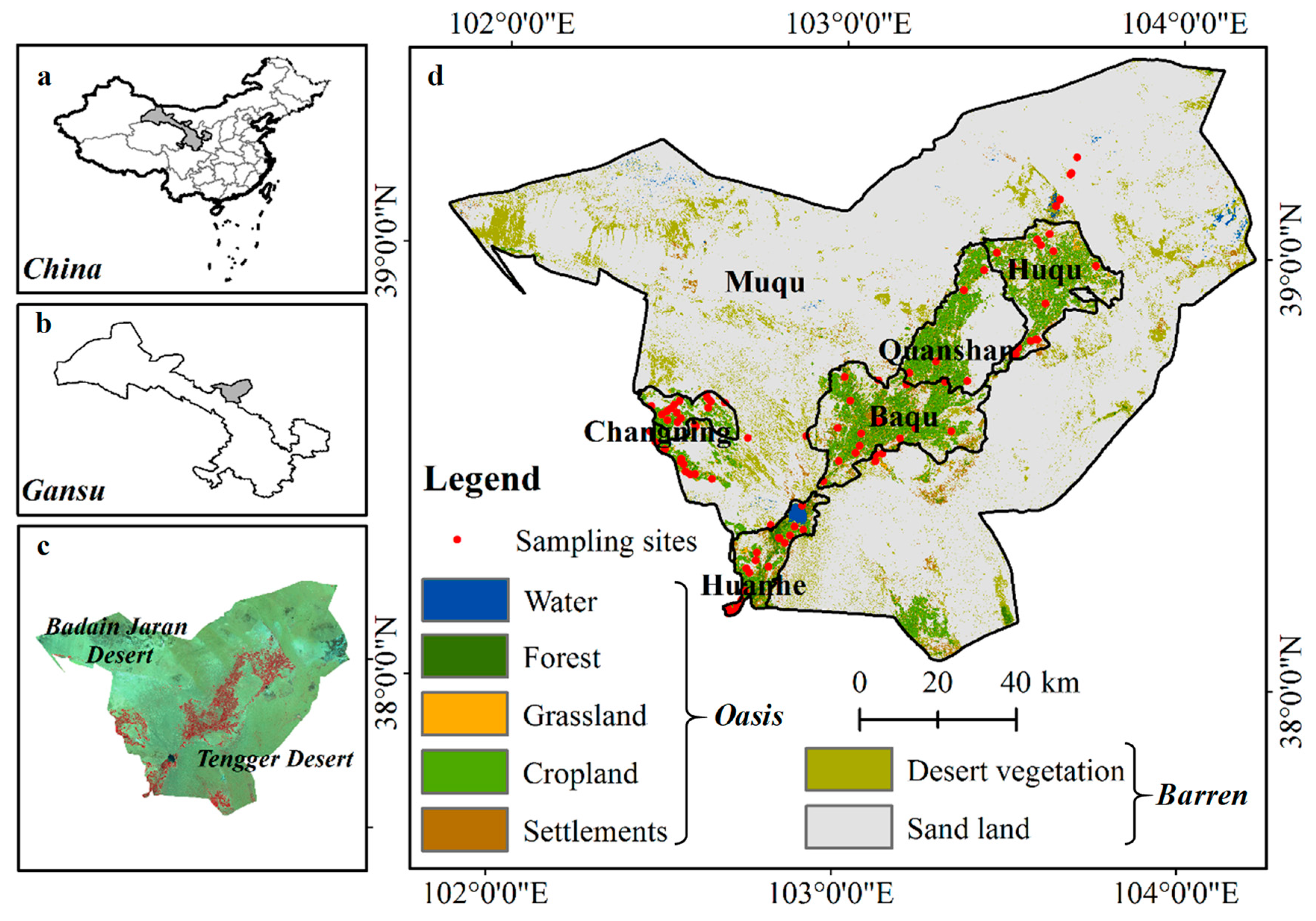
2.1. Study Area

The study area of Minqin (approximately 1.6 × 10⁴ km²) is located in Gansu Province, Northwest China (ranging from 101°49′ to 104°12′ E and from 38°03′ to 39°28′ N, Figure 1), and has an arid continental climate with an average precipitation of about 110 mm; however, accompanied by quite high annual average evaporation of 2664 mm [38]. This study area includes six districts (i.e., Huanhe, Baqu, Quanshan, Huqu, Muqu, and Changning) with diverse dryland landscapes, consisting of oasis and barren areas. The oasis consists predominantly of alluvial plain, including water, forest, grassland, cropland, and settlement, and accounting for about 11.06% of the entire study area, while the remaining 88.94% is covered by the desert vegetation and sand land of the Badain Jaran Desert and Tengger Desert (Figure 1). Within the barren region, Eolian plain is the largest geomorphological type, dominated by the interaction between wind erosion and desert vegetation. The study area is ecologically fragile and infertile, resulting in severe land degradation [39]. Therefore, a series of ecological management measurements have been implemented since the 21st century [38,54]. Spatially-detailed SOM mapping has become one of the primary tasks in this context to reliably evaluate ecological quality and land degradation neutrality at landscape and field scales.

2.2. Methods

The overall workflow of the XWT-based framework for SOM mapping is shown in Figure 2. This framework embodies five Sections, which include (1) soil sampling, (2) XWT features extraction from vegetation and soil-related endmember sequences, (3) XWT features selection as exploratory covariates, (4) model training, validation and robustness, and (5) spatially-detailed SOM mapping and mapping uncertainty evaluation. Detailed descriptions are as follows:

2.2.1. Soil Sampling

We conducted field soil sampling in Minqin from 10 September to 20 September 2016. To match the spatial resolution of commonly used medium and high-resolution satellites (e.g., 30-m Landsat, 16-m GF-1 WFV), soil sampling was implemented in 30 × 30 m square plots [14]. These plots were set across various land use and cover types of the entire study area (Figure 1d). Within each square, 5–6 surface soil profiles were sampled at a 0–20 cm depth and then mixed into one sample to represent each plot’s soil properties. We collected a total of 94 samples for SOM estimates and validation. The Walkley–Black method, commonly determining SOM by quantifying the amount of oxidizable soil carbon as determined by the reaction with acidic dichromate integrated with external heating [55], was used to estimate SOM in the laboratory.

In the study area, the measured SOM ranged from 3.450 g·kg⁻¹ to 34.029 g·kg⁻¹, with an average of 11.992 g·kg⁻¹ (

Table 1. Measured SOM of 94 soil samples.

Land Use/Land Cover	Sample Numbers	Measured SOM (g·kg−1)
		Minimum	Maximum	Average	Standard Error
Desert vegetation	12	3.614	29.853	10.092	7.200
Sand land	16	3.450	11.043	6.112	3.099
Forest	21	4.183	34.029	12.842	7.069
Grassland	6	8.985	17.623	13.237	3.505
Cropland	39	6.938	27.474	14.340	5.534
Total	94	3.450	34.029	11.992	6.037

). Cropland, grassland, and forest in the oasis regions had the highest averaged SOM (14.340 g·kg⁻¹, 13.237 g·kg⁻¹, and 12.842 g·kg⁻¹, respectively), while sand land in the barren areas had only 6.112 g·kg⁻¹ of averaged SOM. As an oasis–desert transitional zone, the averaged SOM of desert vegetation was 10.092 g·kg⁻¹.

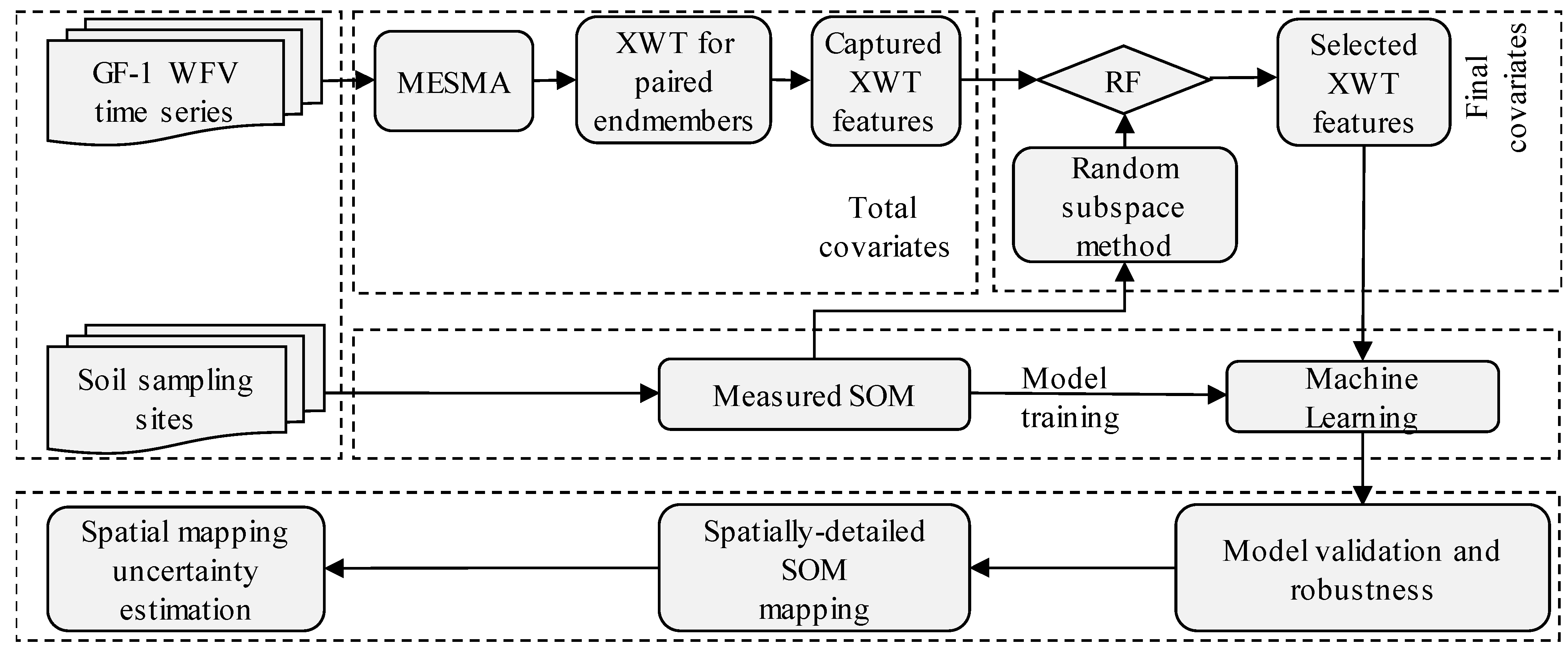
2.2.2. XWT Features Extraction from Endmember Sequences

We used 16-period high-quality GF-1 WFV images from October 2014 to November 2015 when the study area had few clouds. This satellite provided free and high-frequency pretreatment-level radiometric correction products (level 1) with 16-m spatial resolution. The LSMA procedure was proposed to estimate intra-annual GV and soil-related (i.e., SL, SA, and DA) endmember fractions at the 16-m subpixel level [47]. In this measurement, GV represents vegetation photosynthetic foliage, characterized by chlorophyll absorptions in the visible and high reflectance in the near-infrared band, and SL refers to sand in the desert. Similarly, SA is a deterministic element indicating saline land [38,47]. The feature DA contains a fundamental ambiguity resulting from low surface reflectances, caused by the presence of absorptive (black gravel), transmissive (water), or non-illuminated (shade) surfaces [35,38]. Therefore, unmixed vegetation and soil-related endmember fraction sequences offer a continuous representation of land quality in the entire study area [34,35,56]. The details and datasets about LSMA for these four fractional endmembers’ time series can be found in [47].

In addition, the XWT-derived cross-wavelet spectrum, embodying the cross-wavelet power and phase in the temporal space, can quantify interactive information recorded on two related time series of signals in a given wavelet spatial–temporal domain [50]. These cross-wavelet spectrums are efficient approaches for highlighting feedback between multiple time series through XWT features extraction [52,53,57]. In general, XWT is defined as the multiplication of the wavelet spectrum of signal x and the complex conjugate of the wavelet spectrum from signal y,

$$W_{}^{xy}(s)=W_{}^x(s)W_{}^{y*}(s)$$

(1)

represents the cross-wavelet power, and the phase is accordingly defined as

$${\phi }^{xy}(s)=\arctan \frac{\zeta \left\{W^{xy}(s)\right\}}{\theta \left\{W^{xy}(s)\right\}}$$

(2)

where $\zeta \left\{W^{xy}(s)\right\}$ and $\theta \left\{W^{xy}(s)\right\}$ are the imaginary and real components of $W^{xy}(s)$.

Therefore, based on the unmixed vegetation and soil-related endmember fraction time series imageries, the XWT approach was adopted to identify the cross-wavelet power and phase dominating in the intra-annual endmember pairs (i.e., GV and SL, GV and SA, GV and DA) for each pixel. Then, ten ecologically meaningful XWT features (F1 to F10) for each intra-annual endmember pair were calculated from the cross-wavelet power and phase, respectively, following [53].

$$\mathrm{F}1=\frac{{\displaystyle \sum _s{\displaystyle \sum _{n}sn\left|W^{xy}(s)\right|}}}{{\displaystyle \sum _s{\displaystyle \sum _n\left|W^{xy}(s)\right|}}}$$

(3)

$$\mathrm{F}2=\sqrt{\frac{{\displaystyle \sum _s{\displaystyle \sum _n{s}^2{n}^2\left|W^{xy}(s)\right|}}}{{\displaystyle \sum _s{\displaystyle \sum _n\left|W^{xy}(s)\right|}}}}$$

(4)

$$\mathrm{F}3=\frac{{\displaystyle \sum _s{\displaystyle \sum _n\left|W^{xy}(s)\right|}}}{{\left|W^{xy}(s)\right|}_{peak}}$$

(5)

$$\mathrm{F}4=\frac{{\displaystyle \sum _s{\displaystyle \sum _n\left|W^{xy}(s)\right|}}}{\left(s_{\max }-s_{\min }\right)\left(n_{\max }-n_{\min }\right)}$$

(6)

$$\mathrm{F}5=\frac{{\displaystyle \sum _s{\displaystyle \sum _{n}sn\left|{\phi }^{xy}(s)\right|}}}{{\displaystyle \sum _s{\displaystyle \sum _n\left|{\phi }^{xy}(s)\right|}}}$$

(7)

$$\mathrm{F}6=\sqrt{\frac{{\displaystyle \sum _s{\displaystyle \sum _n{s}^2{n}^2\left|{\phi }^{xy}(s)\right|}}}{{\displaystyle \sum _s{\displaystyle \sum _n\left|{\phi }^{xy}(s)\right|}}}}$$

(8)

$$\mathrm{F}7=\frac{{\displaystyle \sum _s{\displaystyle \sum _n\left|{\phi }^{xy}(s)\right|}}}{{\left|{\phi }^{xy}(s)\right|}_{peak}}$$

(9)

$$\mathrm{F}8=\frac{{\displaystyle \sum _s{\displaystyle \sum _n\left|{\phi }^{xy}(s)\right|}}}{\left(s_{\max }-s_{\min }\right)\left(n_{\max }-n_{\min }\right)}$$

(10)

$$\mathrm{F}9=“s”at peak of\left|W^{xy}(s)\right|$$

(11)

$$\mathrm{F}10=“n”at peak of\left|W^{xy}(s)\right|$$

(12)

where F1 and F2, and F5 and F6 are the different normalized forms of the scale- and time-averaged cross-wavelet power and phase, respectively. F3 and F7 indicate the ratio between the summary of the cross-wavelet power and phase and their corresponding peaks, respectively; F4 and F8 are cross-wavelet power and phase, respectively; F9 and F10 represent the scale and time where the cross-wavelet powers peak.

Finally, a total of 30 XWT feature imageries from three coupled intra-annual endmember pairs (i.e., GV and SL, GV and SA, GV and DA) were obtained [53]. Since some machine learning algorithms’ objective functions may be affected by large variability among input covariates [58,59], Min-Max feature scaling was adopted to normalize the range of each independent XWT feature image into the range [0,1]. Thus, 30 normalized XWT feature imageries were obtained as preliminary total covariates in this study. A more detailed description of the XWT-based features derived from endmember sequences can be found in [53].

2.2.3. SOM Exploratory Covariates Selection

The 30 × 30 m sampling plots were relatively matched with the four GF-1 WFV pixels (16-m); we thus collected the average of 2 × 2 pixels of each normalized XWT feature imagery in the geographic sampling plots. The measured SOM and the corresponding 30 normalized XWT features were considered as the predicted variable and possible exploratory covariates, respectively. However, some normalized XWT features may not contribute significant information to the target SOM [60]. Our initial attempt was to filter appropriate covariates conducive to SOM mapping to construct a better training model.

The random forest (RF) method determines the features’ importance in the process of training the regression trees [61,62]. This RF-based feature selection module can select covariates with either linear or nonlinear relationships with the predicted variables. We adopted the RF method to calculate the Gini importance as the criterion of feature selection [63]. However, when any of the correlated exploratory covariates is selected as an important variable in the RF model, the importance of other features will drop sharply [64,65]. Therefore, a random subspace method in the RF model is widely applied to weaken the correlation between features through the random utilization of partial features instead of the entire features [66,67]. Specifically, we employed the entire samples (n = 94) as an input of the random subspace method of the RF model, and 20-fold repetitions were conducted to export the corresponding Gini importance of each XWT feature per repetition. According to average importance of the 20-fold repetitions, we sorted the XWT features from high to low and computed the cumulative contribution to select the features. The Pearson correlation coefficient (r) and significance level (p) between each XWT feature and the measured SOM were calculated with SPSS (Statistical Product and Service Solutions) Version 19.0 to corroborate the features selection results. SPSS is globally recognized as a useful statistical software, currently owned and developed by the International Business Machines Corporation, New York City, NY, United States of America.

2.2.4. State-of-the-Art Machine Learning Approaches for SOM Mapping

In this study, to assess the machine learning approaches that fit our proposed XWT-based framework, four state-of-the-art machine learning models, i.e., ridge regression (RR), least squares-support vector machines (LS-SVM), RF, and gradient boosted regression trees (GBRT), were applied with the selected XWT features for SOM mapping RR is a regression method commonly applied in collinear data analysis [68,69,70]. In essence, it is an improved least squares estimation method for deriving practical and reliable regression coefficients by abandoning the least squares’ unbiasedness at the cost of losing part of the information and decreased regression accuracy. The complexity parameter α is usually selected to control the amount of shrinkage. A larger α relates to higher shrinkage, which corresponds to more robust coefficients of collinearity. Therefore, based on ridge coefficients’ plots as a function of the regularization (Figure S1a), α was set to 10. This parameter resulted in various robust coefficients and intercepts (Figure S1b).

LS-SVM uses equality constraints instead of convex quadratic programming for classical SVMs and provides a convenient Lagrange multiplier solution alpha from simultaneous linear equations [71]. The Gaussian radial basis function was selected as the Kernel function. A grid-search method was used to optimize the C and γ of RBF [72], based on the lowest root mean square error (RMSE) of leave-one-out cross-validation.

RF is a method of classification and prediction. This method is currently the most effective and popular machine learning approach for remotely sensed SOM mapping [24,41]. We developed 100 bagged regression trees with a maximum depth of four at each decision split. The prediction results were considered for the final output of every estimate through mean squared errors as voting criteria [64,73].

GBRT is an iterative decision tree algorithm based on the gradient descent method. It involves the synthesis of various weak classifiers, iteratively trained by increasing the weights of misclassified samples and reducing the weights of accurate samples [74,75]. Here, the least-squares were used to construct the loss profile; we set the number of regression trees, maximum tree depth, and minimum sample segmentation to 200, 3, and 3, respectively. The learning rate was set to 0.05 to avoid fluctuations in the learning profile and over-fitting of the model [63]. The loss profile plot showed that the training and validation sets’ least-squares were close to equilibrium (0.18 and 5.18) after 1000 iterations (Figure S2).

2.2.5. Model Training and Validation

The splitting of sampled data into training and validation sets is regarded as a standard approach to evaluate model performance [14,41]. However, this measurement only indicates model performance for one specific group of split samples and can result in considerable uncertainty [76]. Thus, multiple cross-validations were used to evaluate model performances [41,43]. In previous studies, the number of repetitions varied from 10 to 50. Consequently, in this study, 84% (n = 79) of the soil samples were selected as the training set, and the remaining 16% (n = 15) of the samples were used as the validation set. We also employed a repeated 20-fold cross-validation on our randomly split samples to assess the XWT-based framework’s reliability and efficiency.

For model cross-validation, the coefficient of determination (R²), the root mean square error (RMSE), and the relative percent deviation (RPD) were used as accuracy validation metrics. The first two metrics measure the precision [14,41], while the latter one is used to quantify the estimation reliability of the model for digital soil mapping [77]. They can be formulated as:

$$R^2={\left(\frac{{\displaystyle \sum _{i=1}^n\left(M_i-\overline{M}\right)\left(P_i-\overline{P}\right)}}{\sqrt{{\displaystyle \sum _{i=1}^n{\left(M_i-\overline{M}\right)}^2}}\sqrt{{\displaystyle \sum _{i=1}^n{\left(P_i-\overline{P}\right)}^2}}}\right)}^2$$

(13)

$$RMSE=\sqrt{\frac{{\displaystyle \sum _{i=1}^n{\left(M_i-P_i\right)}^2}}{n}}$$

(14)

$$RPD=\frac{SD}{RMSE}$$

(15)

where $M_i$ and $P_i$ are the measured SOM and predicted SOM, $\overline{M}$ and $\overline{P}$ are averages of the measured SOM and predicted SOM of the training set and validation set, respectively, n is the number of the training set (n = 79) and validation set (n = 15), and SD is the standard deviation of measured SOM. When RPD > 2.0, the model is an excellent index for predicting soil properties; 1.4 < RPD < 2.0 indicates that the predictive model is acceptable, whereas RPD < 1.4 suggests that the reliability of the model is low and cannot be used for prediction [77].

2.2.6. Spatially-Detailed SOM Mapping and Mapping Uncertainty Evaluation

Using a cross-validation model that coupled XWT features with state-of-the-art machine learning approaches, we predicted SOM at the same scale (16-m) as the GF-1 WFV-derived XWT feature images for the entire study area. The averaged SOM at pixel level over the 20 repetitions was calculated as a final mapping result. Mapping uncertainty has been widely adopted in the digital soil mapping domain to ensure SOM mapping stability and reliability [78]. A 90% prediction interval is a common uncertainty specification in digital soil mapping models [78,79]. Therefore, at a 90% prediction interval, we adopted a value of 1.645 times the standard deviation derived from 20 repetitions of SOM mapping results to analyze the mapping of pixel uncertainty for each state-of-the-art machine learning approach.

2.3. Comparisons with Conventional Methods

Studies have explored ways to robustly estimate soil properties from time series of remotely sensed covariates, commonly relying on the arithmetic average of the entire multi-temporal time-series records [43,44]. To confirm the XWT features’ superiority as exploratory covariates, we averaged the values for each endmember in different seasons (i.e., Spring, Summer, Autumn, Winter) and the whole year as covariates to map SOM. In these solutions, using 20 averaged features from multi-temporal endmember sequences, the same validation metrics, i.e., R², RMSE, and RPD, were used to evaluate the predictability and robustness after 20-fold cross-validation. In addition, the trained model of each state-of-the-art machine learning approach was used for spatially-detailed SOM mapping and mapping uncertainty evaluation in the entire study area, as described in Section 2.2.6. The performance of conventionally extracted features was compared with our XWT-based framework.

The two datasets were compared with the estimated SOM in terms of spatial patterns and quantity. They were (1) a 30 × 30 arc-second resolution gridded SOM dataset derived from the China Soil Map of 8979 soil profiles [20], and (2) the improved SOC dataset from SoilGrids at 250-m resolution using a machine learning approach [21]. The SOM and SOC have a linear relationship, hence the SOC dataset from [21] was firstly transformed into SOM multiplying by the empirical coefficient of 1.742 [55]. To quantitatively represent the differences between the existing datasets and our framework, the SOM mapping result was aggregated into the respective spatial resolutions of the two datasets (i.e., 30 × 30 arc-second and 250 × 250 m). Then, we created scatterplots and corresponding fitted curves at the pixel scale of the entire study area.

3. Results

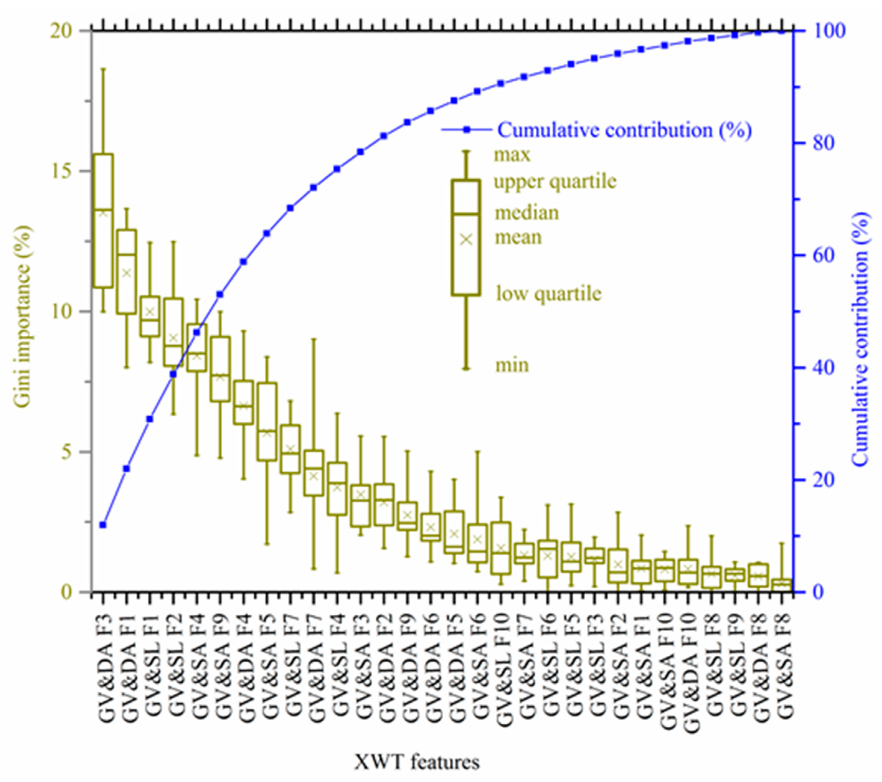
3.1. Selected XWT Features as SOM Covariates

Based on the random subspace method, each XWT feature’s Gini importance and cumulative contribution are displayed in Figure 3. The results revealed that the cumulative contribution of the first 13 XWT features was over 80%. Therefore, these 13 XWT features were selected as final covariates, including GV and DA F1, GV and DA F3, GV and SL F1, GV and SL F2, GV and SA F4, GV and SA F9, GV and DA F4, GV and SA F5, GV and SL F7, GV and DA F7, GV and SL F4, GV and SA F3, and GV and DA F2 (Figure S3).

The XWT feature F1 played a vital role in the RF models, as supported by their Gini importance and relative ranking. F1 consistently ranked as two of the top three variables with the highest importance (>10%, Figure 3). In addition, F2 and F3 had relatively high importance in the RF models (Figure 3). F1, F2, and F3, extracted from the cross wavelet-power of vegetation and soil-related endmember pairs, weighted by the corresponding timescale domain, revealed the degree of intra-annual interactions between vegetation and soil-related endmember sequences. Thus, the three features can reveal the quality of an ecosystem and characterize the content of SOM in the study area. The XWT features refined from the cross wavelet-phase (e.g., F5, F7) were less important in the models, even though they were selected as covariates for SOM mapping (Figure 3). Moreover, it is also noteworthy that feature F9, revealing vegetation phenological regularity, is not a heavily weighted covariate for SOM mapping (Figure 3).

For specific vegetation and soil-related endmember pairs, GV and DA had higher importance than the other two pairs, i.e., GV and SL, and GV and SA. This was demonstrated by the two most important features (i.e., GV and DA F1, GV and DA F3) and a total of five related features of the thirteen selected covariates (Figure 3). Comparatively, despite the XWT features derived from GV and SL, and GV and SA accounting for a large proportion of the selected features (4/13), the contribution of the two pairs was only 24.60% and 22.30%, respectively, considerably less than the contribution of GV and DA (34.32%) (Figure 3). This finding suggested that, unlike the sandy and saline lands with low and homogeneous soil fertility, the greater variability in the interaction of vegetation and dark soil among the landscape types (i.e., cropland, forest, grassland) provided valuable information for accurately characterizing soil fertility attributes.

A linear correlation was found between the measured SOM and some of the selected normalized XWT parameters (GV and DA F1, GV and DA F2, GV and DA F3, GV and SA F3, GV and SA F9, GV and SL F1, GV and SL F2) at the 5% significance level (p < 0.05, Figures S3 and S4). Moreover, some selected normalized XWT features (i.e., GV and SA F4, GV and DA F4, GV and SA F5, GV and SL F7, GV and DA F7, GV and SL F4) had an insignificant linear relationship with the measured SOM (Figures S3 and S4). These features reflect either the average extent of the vegetation–soil interaction (F4) or the presence of phase differences (F5, F7). Therefore, the RF’s random subspace method can effectively identify both valuable linear and nonlinear features and is thus useful for SOM mapping.

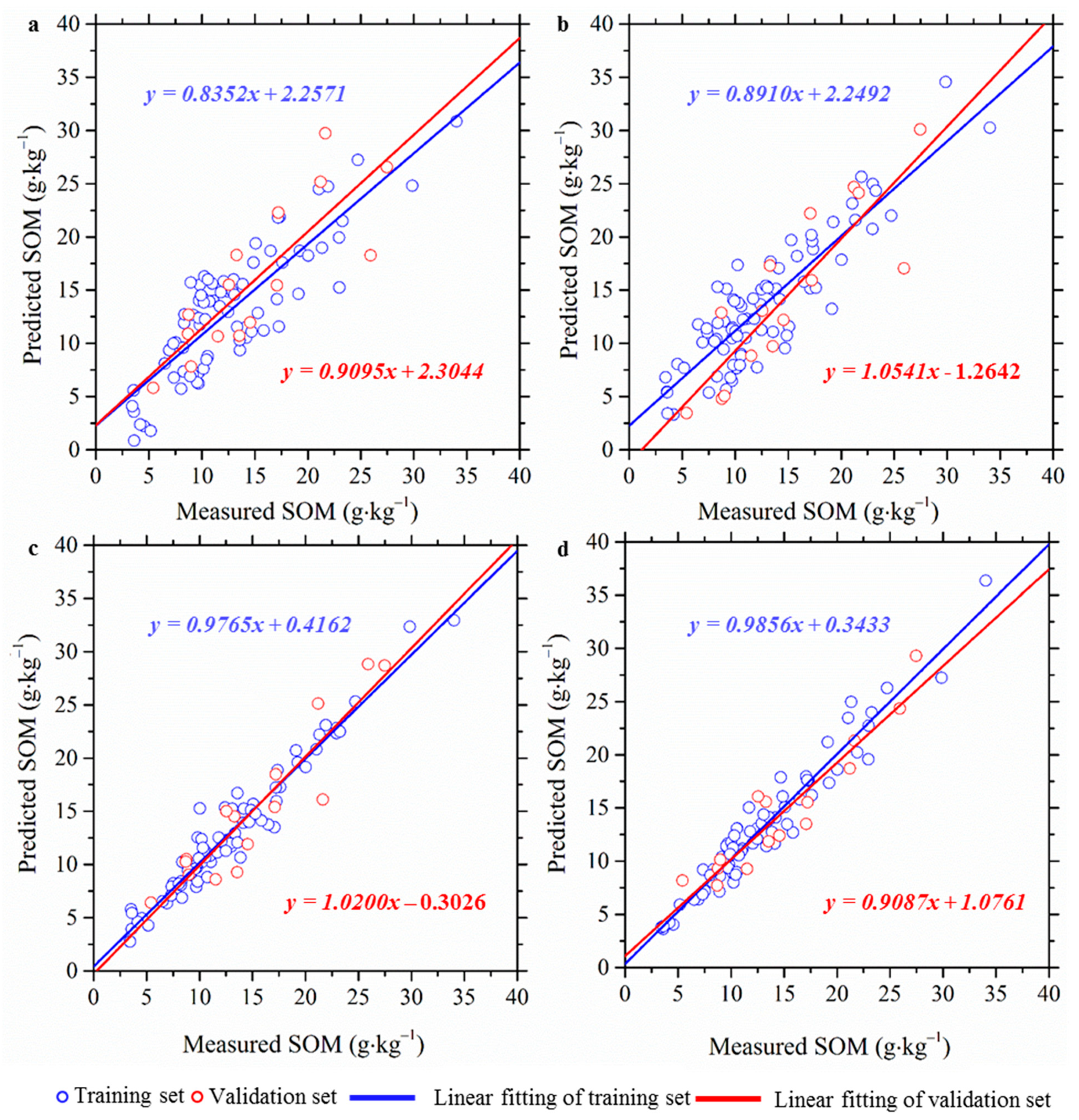
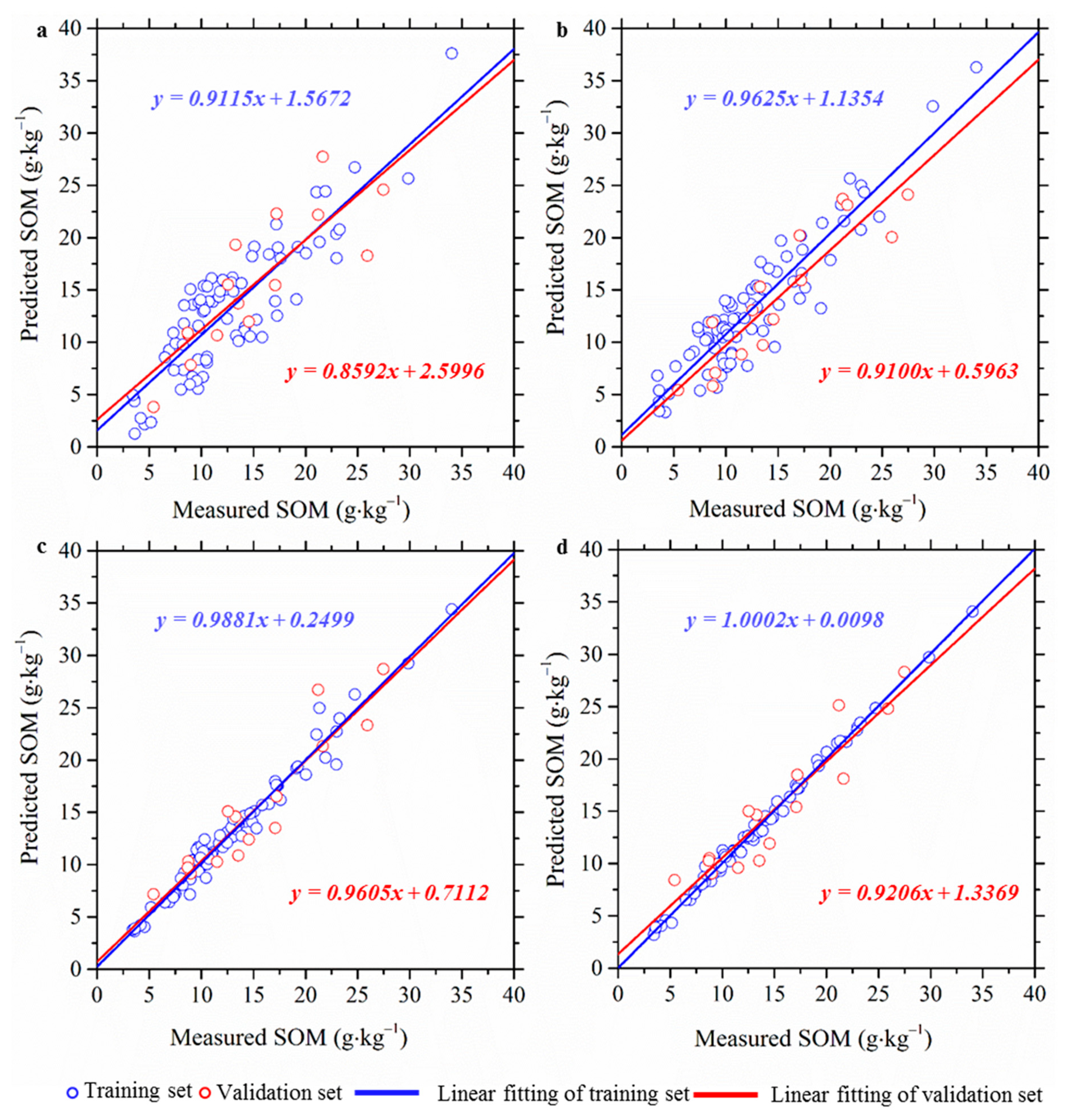
3.2. Performances of XWT-Based Framework

We coupled 13 selected normalized XWT features with state-of-the-art machine learning approaches. The relative performances of the accuracy validation metrics (R², RMSE, and RPD) averaged from the 20 cross-validated models are shown in

Table 2. Evaluation of XWT-based framework in terms of RMSE, R², and RPD through 20-fold cross-validation on our randomly split training set (n = 79) and validation set (n = 16). The average and standard deviation (in brackets) of the accuracy validation metrics were computed for the XWT-based framework, coupled with RR, LS-SVM, RF, and GBRT.

Models	Training Set (n = 79)			Validation Set (n = 15)
	RMSE	R2	RPD	RMSE	R2	RPD
RR	3.148 (2.002)	0.751 (0.401)	1.860 (1.232)	3.635 (2.926)	0.706 (0.321)	1.733 (1.411)
LS-SVM	2.457 (0.987)	0.851 (0.365)	2.385 (1.454)	2.825 (1.354)	0.823 (0.426)	2.231 (1.874)
RF	0.991 (0.051)	0.888 (0.056)	5.913 (0.859)	2.277 (0.621)	0.875 (0.212)	2.729 (1.456)
GBRT	0.427 (0.026)	0.879 (0.012)	13.731 (1.231)	2.309 (0.798)	0.873 (0.198)	2.768 (1.324)

. Both the training and validation sets showed the satisfactory performances of the four state-of-the-art machine learning approaches, as supported by high estimation precisions (R², 0.706–0.875; RMSE, 2.277–3.635) and great reliability (RPD, 1.733–2.729). The better performances of RF and GBRT were indicated by lower RMSE (RF: 2.277, GBRT: 2.309), higher R² (RF: 0.875, GBRT: 0.8738) and RPD (RF: 2.729, GBRT: 2.768), all of which were superior to those of LS-SVM (RMSE: 2.825, R²: 0.823, RPD: 2.231) and RR (RMSE: 3.635, R²: 0.706, RPD: 1.733) (Table 2). These performances were also supported by the relatively small standard deviations of the three accuracy metrics of the RF and GBRT approaches (Table 2). This resulted from the fact that RF and GBRT are able to fully mine both linear and nonlinear information on the selected features. Additionally, the slopes of the fitting curves of the scatter plots of the measured and predicted SOM of RF (0.9605) and GBRT (0.9206) for the validation set were closer to the 1:1 line (Figure 4c,d), also outperforming those of LS-SVM (0.9100) and RR (0.8592). Therefore, RF and GBRT were the most robust SOM estimation approaches in the XWT-based framework.

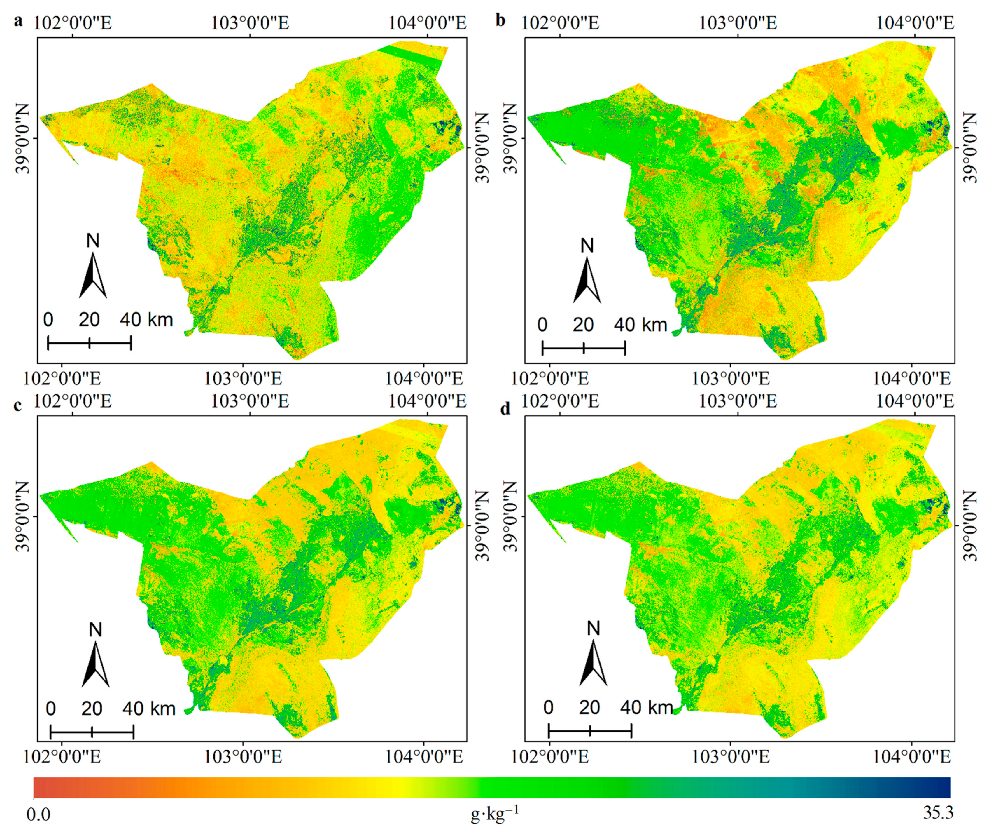
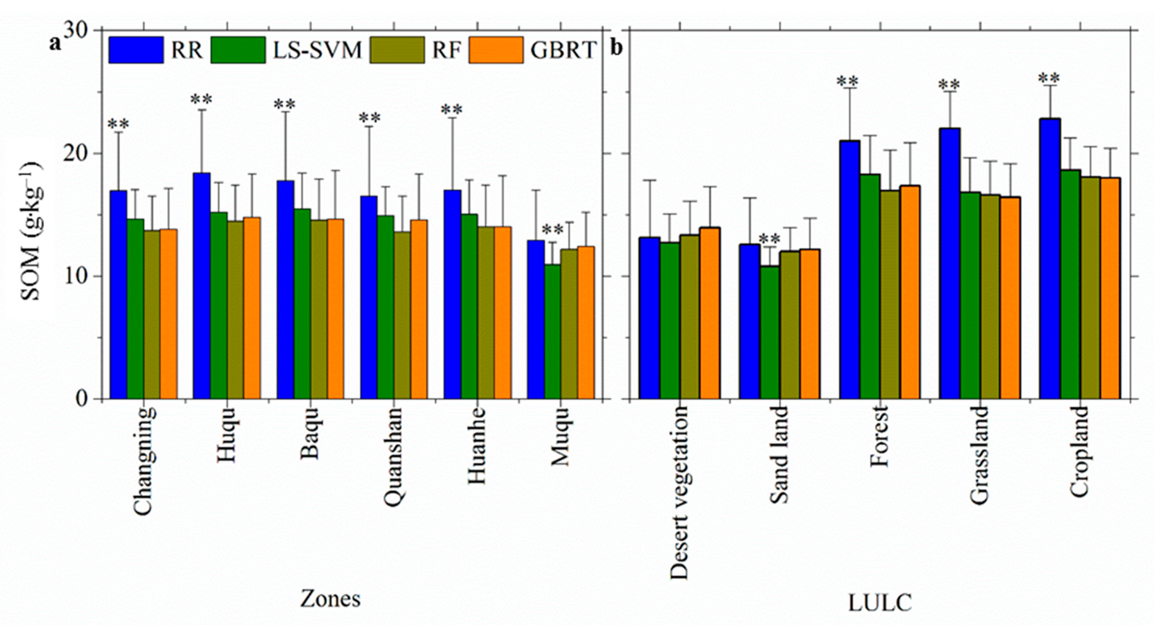
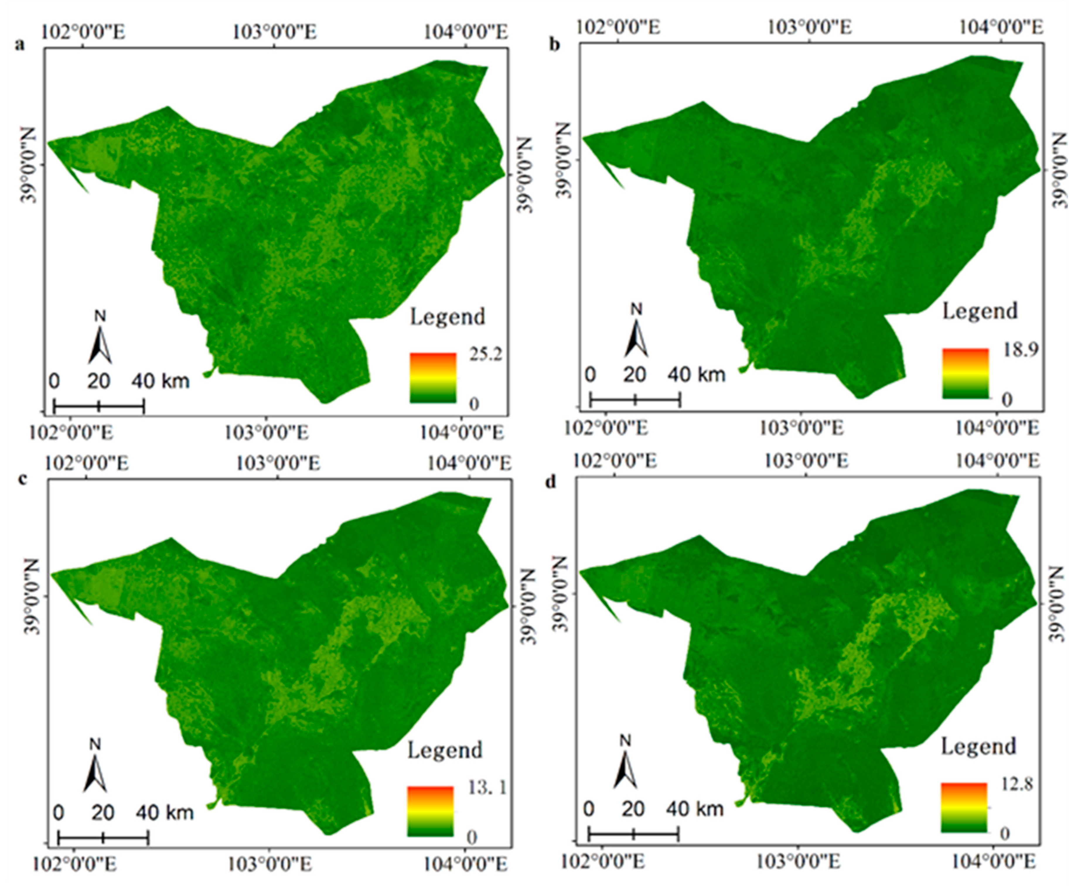
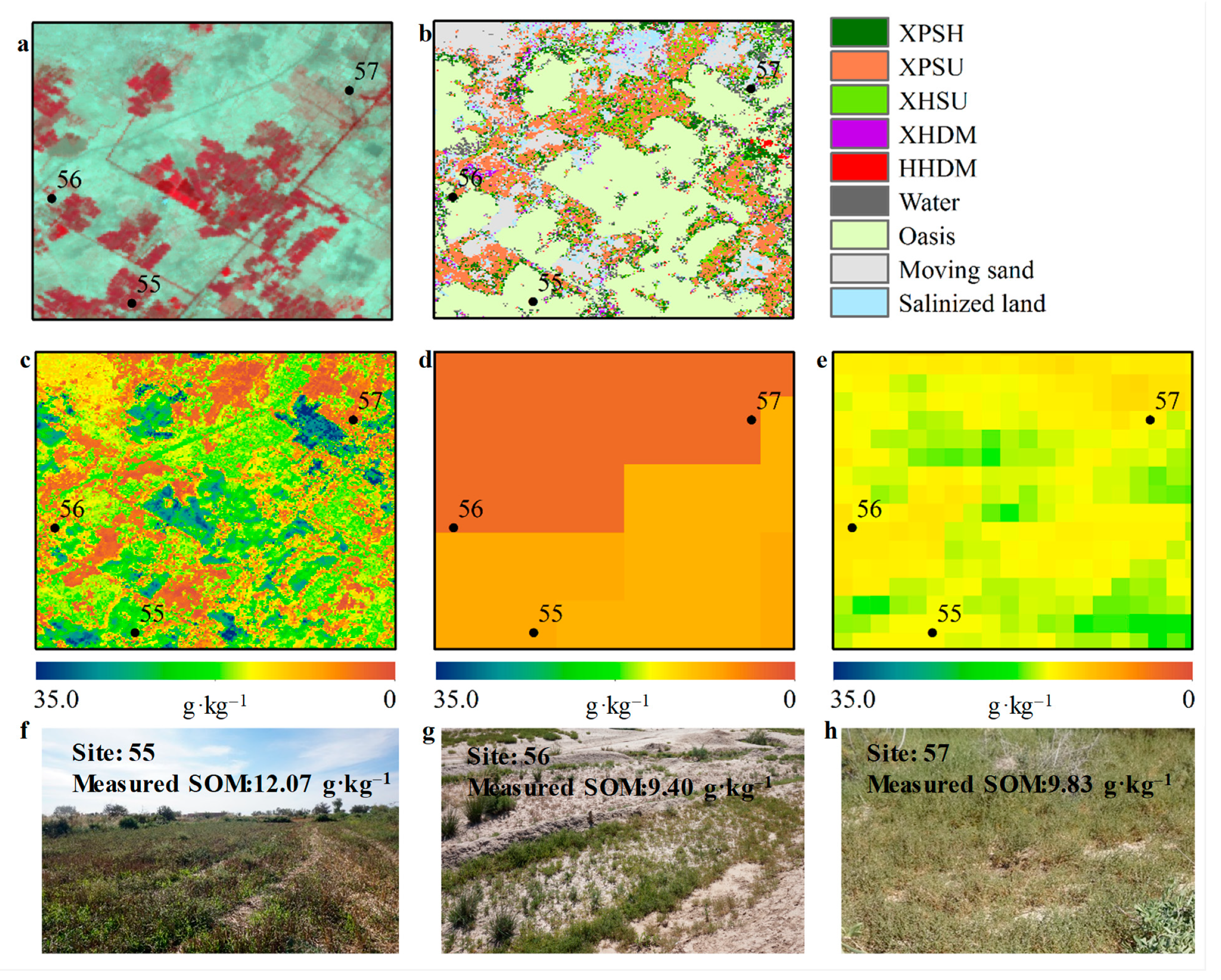
3.3. Spatially-Detailed SOM Mapping and Mapping Uncertainty Evaluation

Using four state-of-the-art machine learning approaches, the predicted continuous spatially-detailed SOM was mapped at fine resolution (16-m). The spatially-detailed averaged SOM maps are shown in Figure 5. The SOM maps display varying patterns of association with the landscapes in the study area. Specifically, the higher SOM (15.01–18.96 g·kg⁻¹) was mostly clustered within the oasis regions (i.e., Changning, Huqu, Baqu, Quanshan, Huanhe) (Figure 5 and Figure 6). These regions are covered by forest, grassland, and cropland but cover only 11.06% of the entire study area (Figure 1). However, regions with lower SOM content are generally found in barren areas, such as scattered small desert vegetation and expansive desert.

In terms of model comparisons, the RF and GBRT approaches provided similar SOM prediction results across different zones, land use, and cover types (Figure 5c,d and Figure 6). The RR approach, however, underestimated the SOM for the oasis areas (forest: 15.01 g·kg⁻¹, grassland: 15.02 g·kg⁻¹, cropland: 16.81 g·kg⁻¹) and sand land (9.58 g·kg⁻¹) at significance levels of 95%, especially in Quanshan (11.93 g·kg⁻¹) and Muqu (9.91 g·kg⁻¹) (Figure 5a and Figure 6). This is proved by the results that the lowest slope of the RR model (0.8592) indicates an underestimation of SOM (Figure 4a), as well as the most unsatisfactory accuracy validation metrics (Table 2). Additionally, the LS-SVM approach also significantly underestimated SOM in Muqu (10.95 g·kg⁻¹) at the 90% significance level (Figure 5b and Figure 6a). This result was mainly attributable to the underestimation of SOM in both desert vegetation (12.73 g·kg⁻¹) and sand land (10.81 g·kg⁻¹) (Figure 6b). As the results suggested, RF and GBRT were the most effective approaches in delineating patterns of SOM.

The spatially continuous mapping uncertainty for each state-of-the-art machine learning approach is shown in Figure 7. We used 1.645 times of the standard deviation derived from 20 repetitions of SOM mapping results as the threshold for evaluating mapping uncertainty at a 90% prediction interval. Consequentially, the mapping uncertainty of RR, LS-SVM, RF, and GBRT in the study area were in the range of 0–25.2 g·kg⁻¹, 0–18.9 g·kg⁻¹, 0–13.1 g·kg⁻¹, and 0–12.8 g·kg⁻¹, respectively (Figure 7). The mapping uncertainty histograms (Figure S5) indicated that the mapping uncertainty of the XWT-based framework ranged from 0–5 g·kg⁻¹, representing relatively low averaged uncertainty for all the machine learning approaches, i.e., RR (2.101 ± 1.184), LS-SVM (1.708 ± 1.016), RF (1.665 ± 0.816) and GBRT (1.845 ± 1.410). Compared to the barren region with relatively lower SOM, the oasis regions had higher mapping uncertainty of the XWT-based framework approaches. The mapping uncertainty of RF was slightly superior to the other models (Figure S5).

Overall, by coupling 13 selected XWT features with the RF and GBRT approaches, we successfully applied the XWT-based framework to map SOM with superior accuracy and robustness. Therefore, we suggest selecting the two approaches as the optimal SOM mapping model when coupled with XWT features.

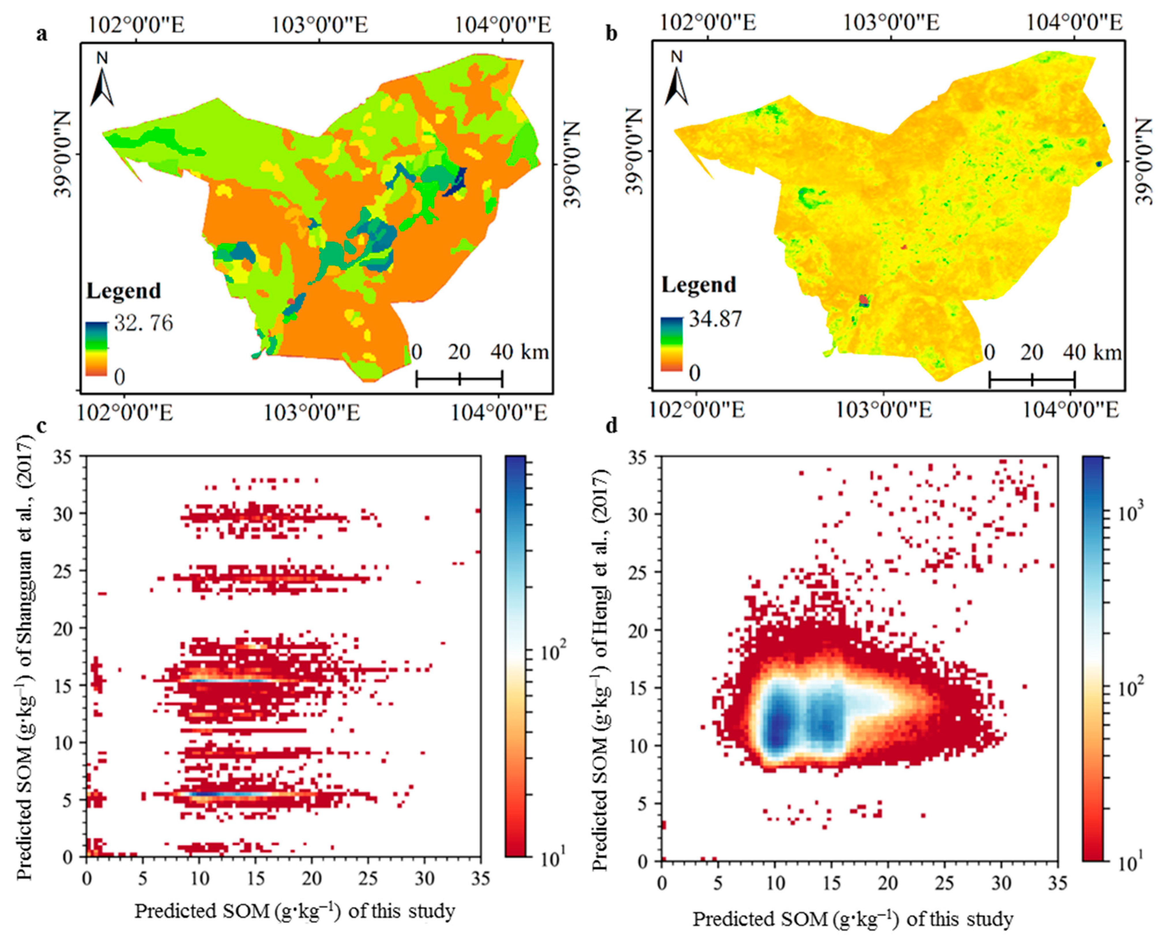
3.4. Comparisons with Other Features and Existing Datasets

Using the 20 averaged value for four endmembers in different seasons (i.e., Spring, Summer, Autumn, Winter) and the whole year as covariates, both the accuracy and reliability were inferior to those derived when using the XWT-framework. There were higher RMSE (4.001, 3.258, 2.406, 2.655), lower R² (0.689, 0.770, 0.854, 0.828) and RPD (1.575, 1.836, 2.325, 2.307) for RR, LS-SVM, RF, and GBRT, respectively (

Table 3. Evaluation results of SOM estimation based on conventionally averaged covariates in terms of RMSE, R², and RPD, after 20 iterations with the same training and validation sets as the XWT features. Average and standard deviations are shown within parenthesis.

Models	Training Set (N = 79)			Validation Set (N = 15)
	RMSE	R2	RPD	RMSE	R2	RPD
RR	3.288 (2.961)	0.731 (0.624)	1.782 (1.222)	4.001 (4.565)	0.689 (0.671)	1.575 (1.687)
LS-SVM	2.493 (1.824)	0.795 (0.599)	1.991 (1.416)	3.258 (3.954)	0.770 (0.610)	1.836 (1.600)
RF	1.299 (0.141)	0.831 (0.242)	3.458 (1.211)	2.406 (1.645)	0.845 (0.492)	2.325 (1.723)
GBRT	1.202 (0.107)	0.856 (0.190)	6.459 (1.200)	2.655 (2.470)	0.828 (0.666)	2.307 (1.820)

). These large differences between the XWT features and the arithmetically averaged covariates resulted in more dispersed scatter plots between the measured and predicted SOM for both the training and validation sets (Figure 8). Regardless of the machine learning method, large variances were observed in the SOM mapping in the entire study area between the two sets of covariate inputs (Figure 5 and Figure S6). Accompanied by the higher standard deviation of RMSE, R², and RPD (Table 3), the conventionally averaged covariates-based models showed higher variability, resulting in greater averaged mapping uncertainty for RR (5.802 ± 2.921), LS-SVM (4.485 ± 2.706), RF (3.171 ± 1.839), and GBRT (3.200 ± 2.251) in the entire study area (Figure 7 and Figure S7). Compared to the averaged covariates of a single-season and the whole year, the XWT highlights continuous information in space and time domains and quantifies weighted interactive information, recorded on two related time-series signals.

We also found that our 16-m spatially-detailed SOM results can provide more spatial details and patterns compared to the two existing datasets (Figure 9 and Figure 10). Although linear relationships existed between our SOM map and the two existing datasets, in the whole area, the similar clusters with discrete values in the existing datasets were corrected with continuous values by our SOM model (Figure 9c). Moreover, some interesting findings were observed. First, in the areas with high fractions of soil exposure, common in deserts, the two existing datasets had a number of SOM with <5 g·kg⁻¹, especially for the 30 × 30 arc-second resolution gridded SOM dataset (Figure 9). Second, within regions with low vegetation cover fractions, particularly desert vegetation (e.g., sampling plot 57), the vegetation coverage provided incorrect information for SOM estimation, instead of serious sandy and salinized soil. Thus, the performance of the SoilGrids dataset overestimated SOM in the barren region, in which SOM was ~10 g·kg⁻¹. Third, SOM maps are underestimated by both datasets within oasis regions (e.g., sampling plot 56, Figure 10b–f). Therefore, in heterogeneous landscapes, the XWT-based SOM map weighted the characteristics of the inter-annual vegetation and soil-related endmember pairs and produced an accurately continuous SOM estimation (Figure 9 and Figure 10).

4. Discussion

4.1. Remotely Sensed Soil–Vegetation Interaction with XWT for Digital Soil Mapping

Benefitting from continuous observation of the earth’s surface, remotely sensed imageries have been proven to support the spatial interpolation of sparsely sampled soil property data [16,17,18,19,20,21]. The spatial resolution of imagery determines the spatial refinement of digital soil mapping. This is mainly due to the fact that a pixel of remote sensing imagery usually represents comprehensive information of the land surface within such an extent. High-resolution GF-1 WFV images (16-m) used in this paper are important for capturing the spatial variability of dryland systems for SOM mapping, and thus support spatially-detailed dryland soil organic matter mapping. In addition, enriched and appropriated variables derived from remote sensing data improved the accuracy of the digital soil mapping. Although various studies have been dedicated to feature exploitation and optimization from spatiotemporal spectral indexes and other environmental features [22,23,24,25,26,27,28,43,44], the detailed information from time series of subpixel fractions that was proven to be robust and reliable in this study has not been unearthed and discussed in previous studies.

4.1.1. Soil–Vegetation Interaction Contributed to Digital Soil Mapping

Soil and vegetation are prominent components of natural ecosystems and interact and affect each other [80]. This feedback results in predictable measurements of soil properties by using vegetation and soil distributions as the covariate. In previous studies, an integrated LSMA framework considering both apparent vegetation and soil was recommended to identify dynamic land quality processes in dryland systems [14]. The vegetation and soil-related endmember fractions offer a better understanding of the related biophysical processes [81] and contain more information, compared to susceptible vegetation indices [47]. Therefore, our results demonstrated that both fractional soil and vegetation information can capture the complex surface attributes and processes in spatiotemporal heterogeneous barren areas, in which the presence of soil background has a huge influence on vegetation indices [29,30,82]. These results corrected the overestimation of vegetation indices-driven SOM mapping (Figure 9 and Figure 10). In addition, the detailed information of soil–vegetation interaction can mitigate the saturation effect of remotely sensed vegetation indices in high vegetation coverage areas, without enough differentiated vegetation information [30], and improve mapping accuracy in the underestimated oasis regions (Figure 9 and Figure 10). We thus verified that the soil–vegetation interaction was sufficient to serve as a fundamental basis for biophysical and biogeochemical SOM mapping in dryland systems. These findings were confirmed by the outcome of SOM mapping and state measurement using three sparse-temporal vegetation and soil-related endmembers and environmental covariates, in Minqin County, at the same scale as the Landsat data [14]. In addition, the vegetation and soil-related endmember fractions can be standardized for the inter-comparison of estimates from different sensors across space and time [35], which would provide migration conditions for digital soil mapping across space, time, and sensors.

4.1.2. XWT-Based Time-Series Features Extraction for Digital Soil Mapping

The XWT provides a synthetic insight into the structure of signals interaction in continuous space and time domains [83,84], as well as the weighted interactive characteristics of wavelet coefficients recorded on two related time series of signals [50,53]. The results suggested that XWT’s interactive features provided detailed SOM representations in dryland systems like Minqin. Therefore, the XWT features perform better than arithmetically averaged covariates at diverse temporal scales, as well as the previous study, with three sparse-temporal vegetation and soil-related endmembers in Minqin at the same scale as Landsat (RMSE = 4.36, [14]).

Substantial evidence supports the notion that SOM dynamics are more susceptible to the total amount of vegetation biomass input and its accumulation and loss processes [85,86,87]. Hence, both vegetation productivity across a given year and soil physical properties play important roles in regulating the accumulation and loss of SOM in natural ecosystems [87,88]. The observed interactive patterns between vegetation and soil represent critical land surface processes affecting SOM, and in turn, responding to SOM. Therefore, the XWT features that revealed temporally interactive degrees of vegetation and soil-related endmember pairs across continuous temporal and spatial domains (F1-F3) played a crucial role in SOM mapping (Figure 3). Although previous evidence underscored the importance that timing corresponds to the peak of vegetation growth (F9) to help identify different land cover types [53], this feature did not play a decisive role in the mapping of SOM (Figure 3). This may be explained by the fact that vegetation’s phenological change is primarily driven by climate [89,90,91] instead of soil fertility. Moreover, the XWT features refined from the cross wavelet-phase (e.g., F5, F7) were less important (Figure 3); however, these features reflect a nonlinear process between SOM and the surface vegetation–soil interaction (Figure S4). These results suggested that known interrelationships between factors in the soil environment could provide a reasonable explanation for the comparable strength of the models with unique sets of predictor variables and would be beneficial for digital soil mapping over regions where base maps are limited.

4.2. Future Applications and Outlook

Our study proved that temporally interactive features extracted with XWT methods play an important role in SOM mapping, although some limitations and corresponding outlooks in the domain of digital soil mapping exist. In terms of digital soil mapping solutions, time-series of remote sensing data at different spatial and temporal scales can further improve the prediction of surface SOM [92]. Accordingly, more in-depth and extensive tests of the utility of long-term remotely sensed vegetation and soil fractions were suggested for predicting SOM across various soil depths, as well as diverse ecosystems. In addition, with the continuous development of high-frequency satellites and the progress of space–time fusion technology [53,93], the XWT can extract more useful information from high temporal and spatial vegetation and soil cubes.

For the application of spatially-detailed SOM mapping in dryland systems, multi-temporal land use/cover changes derived from LSMA can provide information about land degradation and help establish restoration strategies [39,94,95]. For example, land degradation (desertification and salinization) and its associated land cover types can be estimated by combining the land use and cover with fractions of vegetation and soil-related endmembers [95]. As a key variable characterizing soil structure and function, SOM can estimate the processing of land degradation in dryland systems [2,14]. SOM assessments integrated with terrestrial vegetation primary production parameters, i.e., gross primary productivity and net primary productivity, are attracting the attention of scientists and governments for land degradation neutrality evaluation and monitoring [7,96,97,98,99]. Thus, the spatially-detailed SOM derived in this study provides an opportunity to assess the land degradation neutrality status of dryland systems and offers interpretable land degradation knowledge for sustainable management.

5. Conclusions

In this study, we demonstrated the efficacy and reliability of the proposed novel XWT-based framework in predicting SOM in a dryland system of Northwest China. We first extracted ecologically meaningful XWT features from interactive intra-annual vegetation and soil-related endmember sequences and then filtered valuable XWT features as final exploratory covariates for SOM mapping. Using 13 selected XWT features, we successfully applied this framework to map SOM, coupled with the RF and GBRT approaches, with superior accuracy and robustness indicated by lower RMSE, higher R², and RPD, as well as lower uncertainty. Furthermore, the XWT-based framework outperformed the arithmetic average based models, as evidenced by the lower RMSE and improved R² and RPD of the validation set and the lower estimation uncertainty for four state-of-the-art machine learning approaches. Meanwhile, our proposed framework provided accurate high-spatial SOM maps compared to existing datasets. We highlighted how XWT offers superior accuracy and robustness for SOM mapping. XWT can characterize the intra-annual feedback between vegetation and soil-related endmember sequences at a high temporal and spatial resolution. Moreover, our findings of the soil–vegetation feedback contribution to SOM, advance an improved understanding of soil properties and regional ecological quality in dryland systems and provide an opportunity to assess land degradation neutrality at landscape and field scales.

References

1. Middleton, N.; Thomas, D. World Atlas of Desertification; Oxford University Press: Oxford, UK, 1997. [Google Scholar]
2. Reynolds, J.F.; Smith, D.M.S.; Lambin, E.F.; Turner, B.L.; Mortimore, M.; Batterbury, S.P.; Downing, T.E.; Dowlatabadi, H.; Fernández, R.J.; Herrick, J.E.; et al. Global Desertification: Building a Science for Dryland Development. Science 2007, 316, 847–851. [Google Scholar] [CrossRef] [PubMed] [Green Version]
3. Safriel, U.; Adeel, Z.; Niemeijer, D.; Puigdefabregas, J.; White, R.; Lal, R.; Winslow, M.; Ziedler, J.; Prince, S.; Archer, E.; et al. Dryland Systems, Ecosystems and Human Well-Being: Current State and Trends. Findings of the Condition and Trends Working Group; Island Press: Washington, DC, USA, 2020; pp. 623–662. [Google Scholar]
4. Giuliani, G.; Mazzetti, P.; Santoro, M.; Nativi, S.; Van Bemmelen, J.; Colangeli, G.; Lehmann, A. Knowledge generation using satellite earth observations to support sustainable development goals (SDG): A use case on Land degradation. Int. J. Appl. Earth Obs. Geoinf. 2020, 88, 102068. [Google Scholar] [CrossRef]
5. UN Convention to Combat Desertification (UNCCD). A Stronger UNCCD for a Land-Degradation Neutral World; Issue Brief; UNCCD: Bonn, Germany, 2013. [Google Scholar]
6. Orr, B.J.; Cowie, A.L.; Castillo Sanchez, V.M.; Chasek, P.; Crossman, N.D.; Erlewein, A.; Louwagie, G.; Maron, M.; Metternicht, G.I.; Minelli, S. Scientific conceptual framework for land degradation neutrality. In A Report of the Science-Policy Interface; United Nations Convention to Combat Desertification (UNCCD): Bonn, Germany, 2017. [Google Scholar]
7. Cowie, A.L.; Orr, B.J.; Sanchez, V.M.C.; Chasek, P.; Crossman, N.D.; Erlewein, A.; Louwagie, G.; Maron, M.; Metternicht, G.I.; Minelli, S.; et al. Land in balance: The scientific conceptual framework for Land Degradation Neutrality. Environ. Sci. Policy 2018, 79, 25–35. [Google Scholar] [CrossRef]
8. Altieri, M.A. The ecological role of biodiversity in agroecosystems. Agric. Ecosyst. Environ. 1999, 74, 19–31. [Google Scholar] [CrossRef] [Green Version]
9. Lehmann, J.; Kleber, M. The contentious nature of soil organic matter. Nature 2015, 528, 60–68. [Google Scholar] [CrossRef]
10. Parry, M.; Parry, M.L.; Canziani, O.; Palutikof, J.; Van der Linden, P.; Hanson, C. Climate Change 2007-Impacts, Adaptation and Vulnerability: Working Group II Contribution to the Fourth Assessment Report of the IPCC; Cambridge University Press: Cambridge, UK, 2007. [Google Scholar]
11. Pan, G.; Smith, P.; Pan, W. The role of soil organic matter in maintaining the productivity and yield stability of cereals in China. Agric. Ecosyst. Environ. 2009, 129, 344–348. [Google Scholar] [CrossRef]
12. Schmidt, M.W.I.; Torn, M.S.; Abiven, S.; Dittmar, T.; Guggenberger, G.; Janssens, I.A.; Kleber, M.; Kögel-Knabner, I.; Lehmann, J.; Manning, D.A.C.; et al. Persistence of soil organic matter as an ecosystem property. Nature 2011, 478, 49–56. [Google Scholar] [CrossRef] [Green Version]
13. Tiessen, H.; Cuevas, E.; Chacón, P. The role of soil organic matter in sustaining soil fertility. Nature 1994, 371, 783–785. [Google Scholar] [CrossRef]
14. Sun, D.; Zhang, P.; Sun, Q.; Jiang, W. A dryland cover state mapping using catastrophe model in a spectral endmember space of OLI: A case study in Minqin, China. Int. J. Remote Sens. 2019, 40, 5673–5694. [Google Scholar] [CrossRef]
15. Minasny, B.; Malone, B.P.; McBratney, A.; Angers, D.A.; Arrouays, D.; Chambers, A.; Chaplot, V.; Chen, Z.-S.; Cheng, K.; Das, B.S.; et al. Soil carbon 4 per mille. Geoderma 2017, 292, 59–86. [Google Scholar] [CrossRef]
16. Ben-Dor, E.; Chabrillat, S.; Demattê, J.A.M.; Taylor, G.R.; Hill, J.; Whiting, M.L.; Sommer, S. Using imaging spectroscopy to study soil properties. Remote Sens. Environ. 2009, 113 (Suppl. 1), S38–S55. [Google Scholar] [CrossRef]
17. Zhang, M.; Liu, H.; Zhang, M.; Yang, H.; Jin, Y.; Han, Y.; Tang, H.; Zhang, X.; Zhang, X. Mapping Soil Organic Matter and Analyzing the Prediction Accuracy of Typical Cropland Soil Types on the Northern Songnen Plain. Remote Sens. 2021, 13, 5162. [Google Scholar] [CrossRef]
18. Mulder, V.; de Bruin, S.; Schaepman, M.; Mayr, T. The use of remote sensing in soil and terrain mapping—A review. Geoderma 2011, 162, 1–19. [Google Scholar] [CrossRef]
19. Zhang, M.; Zhang, M.; Yang, H.; Jin, Y.; Zhang, X.; Liu, H. Mapping Regional Soil Organic Matter Based on Sentinel-2A and MODIS Imagery Using Machine Learning Algorithms and Google Earth Engine. Remote Sens. 2021, 13, 2934. [Google Scholar] [CrossRef]
20. Shangguan, W.; Dai, Y.; Liu, B.; Zhu, A.; Duan, Q.; Wu, L.; Ji, D.; Ye, A.; Yuan, H.; Zhang, Q.; et al. A China data set of soil properties for land surface modeling. J. Adv. Model. Earth Syst. 2013, 5, 212–224. [Google Scholar] [CrossRef]
21. Hengl, T.; De Jesus, J.M.; Heuvelink, G.B.M.; Gonzalez, M.R.; Kilibarda, M.; Blagotić, A.; Shangguan, W.; Wright, M.N.; Geng, X.; Bauer-Marschallinger, B.; et al. SoilGrids250m: Global gridded soil information based on machine learning. PLoS ONE 2017, 12, e0169748. [Google Scholar] [CrossRef] [PubMed] [Green Version]
22. Guo, L.; Fu, P.; Shi, T.; Chen, Y.; Zhang, H.; Meng, R.; Wang, S. Mapping field-scale soil organic carbon with unmanned aircraft system-acquired time series multispectral images. Soil Tillage Res. 2020, 196, 104477. [Google Scholar] [CrossRef]
23. Luo, C.; Zhang, X.; Meng, X.; Zhu, H.; Ni, C.; Chen, M.; Liu, H. Regional mapping of soil organic matter content using multitemporal synthetic Landsat 8 images in Google Earth Engine. CATENA 2022, 209, 105842. [Google Scholar] [CrossRef]
24. Guo, P.-T.; Li, M.-F.; Luo, W.; Tang, Q.-F.; Liu, Z.-W.; Lin, Z.-M. Digital mapping of soil organic matter for rubber plantation at regional scale: An application of random forest plus residuals kriging approach. Geoderma 2015, 237, 49–59. [Google Scholar] [CrossRef]
25. Luo, C.; Wang, Y.; Zhang, X.; Zhang, W.; Liu, H. Spatial prediction of soil organic matter content using multiyear synthetic images and partitioning algorithms. CATENA 2022, 211, 106023. [Google Scholar] [CrossRef]
26. Liang, Z.; Chen, S.; Yang, Y.; Zhao, R.; Shi, Z.; Viscarra, R.R.A. Baseline map of soil organic matter in china and its associated uncertainty. Geoderma 2019, 335, 47–56. [Google Scholar] [CrossRef]
27. Wang, S.; Fan, J.; Zhong, H.; Li, Y.; Zhu, H.; Qiao, Y.; Zhang, H. A multi-factor weighted regression approach for estimating the spatial distribution of soil organic carbon in grasslands. CATENA 2019, 174, 248–258. [Google Scholar] [CrossRef]
28. Tayebi, M.; Rosas, J.F.; Mendes, W.; Poppiel, R.; Ostovari, Y.; Ruiz, L.; dos Santos, N.; Cerri, C.; Silva, S.; Curi, N.; et al. Drivers of Organic Carbon Stocks in Different LULC History and along Soil Depth for a 30 Years Image Time Series. Remote Sens. 2021, 13, 2223. [Google Scholar] [CrossRef]
29. Baret, F.; Guyot, G. Potentials and limits of vegetation indices for LAI and APAR assessment. Remote Sens. Environ. 1991, 35, 161–173. [Google Scholar] [CrossRef]
30. Huete, A.R. A soil-adjusted vegetation index (SAVI). Remote Sens. Environ. 1988, 25, 295–309. [Google Scholar] [CrossRef]
31. Sankey, T.T.; Weber, K.T. Rangeland Assessments Using Remote Sensing: Is NDVI Useful. Final Report: Comparing Effects of Management Practices on Rangeland Health with Geospatial Technologies; NNX06AE47G: Pocatello, ID, USA, 2009; p. 168. [Google Scholar]
32. Smith, W.K.; Dannenberg, M.P.; Yan, D.; Herrmann, S.; Barnes, M.L.; Barron-Gafford, G.A.; Biederman, J.A.; Ferrenberg, S.; Fox, A.M.; Hudson, A.; et al. Remote sensing of dryland ecosystem structure and function: Progress, challenges, and opportunities. Remote Sens. Environ. 2019, 233, 111401. [Google Scholar] [CrossRef]
33. Adams, J.B.; Smith, M.O.; Johnson, P.E. Spectral mixture modeling: A new analysis of rock and soil types at the Viking Lander 1 Site. J. Geophys. Res. Earth Surf. 1986, 91, 8098–8112. [Google Scholar] [CrossRef]
34. Roberts, D.; Smith, M.; Adams, J. Green vegetation, nonphotosynthetic vegetation, and soils in AVIRIS data. Remote Sens. Environ. 1993, 44, 255–269. [Google Scholar] [CrossRef]
35. Small, C. The Landsat ETM+ spectral mixing space. Remote Sens. Environ. 2004, 93, 1–17. [Google Scholar] [CrossRef]
36. Van Der Meer, F. Spectral unmixing of Landsat Thematic Mapper data. Int. J. Remote Sens. 1995, 16, 3189–3194. [Google Scholar] [CrossRef]
37. Dawelbait, M.; Morari, F. Monitoring desertification in a Savannah region in Sudan using Landsat images and spectral mixture analysis. J. Arid Environ. 2012, 80, 45–55. [Google Scholar] [CrossRef]
38. Sun, D.; Liu, N. Coupling spectral unmixing and multiseasonal remote sensing for temperate dryland land-use/land-cover mapping in Minqin County, China. Int. J. Remote Sens. 2015, 36, 3636–3658. [Google Scholar] [CrossRef]
39. Sun, D. Detection of dryland degradation using Landsat spectral unmixing remote sensing with syndrome concept in Minqin County, China. Int. J. Appl. Earth Obs. Geoinf. 2015, 41, 34–45. [Google Scholar] [CrossRef]
40. Sun, D.; Jiang, W. Agricultural Soil Alkalinity and Salinity Modeling in the Cropping Season in a Spectral Endmember Space of TM in Temperate Drylands, Minqin, China. Remote Sens. 2016, 8, 714. [Google Scholar] [CrossRef] [Green Version]
41. Wang, B.; Waters, C.; Orgill, S.; Cowie, A.; Clark, A.; Liu, D.L.; Simpson, M.; McGowen, I.; Sides, T. Estimating soil organic carbon stocks using different modelling techniques in the semi-arid rangelands of eastern Australia. Ecol. Indic. 2018, 88, 425–438. [Google Scholar] [CrossRef]
42. Stavros, E.N.; Schimel, D.; Pavlick, R.; Serbin, S.; Swann, A.; Duncanson, L.; Fisher, J.B.; Fassnacht, F.; Ustin, S.; Dubayah, R.; et al. ISS observations offer insights into plant function. Nat. Ecol. Evol. 2017, 1, 194. [Google Scholar] [CrossRef] [PubMed]
43. Maynard, J.J.; Levi, M.R. Hyper-temporal remote sensing for digital soil mapping: Characterizing soil-vegetation response to climatic variability. Geoderma 2017, 285, 94–109. [Google Scholar] [CrossRef] [Green Version]
44. Wilson, C.H.; Caughlin, T.T.; Rifai, S.W.; Boughton, E.H.; Mack, M.C.; Flory, S.L. Multi-decadal time series of remotely sensed vegetation improves prediction of soil carbon in a subtropical grassland. Ecol. Appl. 2017, 27, 1646–1656. [Google Scholar] [CrossRef]
45. Yang, R.-M.; Guo, W.-W. Modelling of soil organic carbon and bulk density in invaded coastal wetlands using Sentinel-1 imagery. Int. J. Appl. Earth Obs. Geoinf. 2019, 82, 101906. [Google Scholar] [CrossRef]
46. Zhang, Y.; Guo, L.; Chen, Y.; Shi, T.; Luo, M.; Ju, Q.; Zhang, H.; Wang, S. Prediction of Soil Organic Carbon based on Landsat 8 Monthly NDVI Data for the Jianghan Plain in Hubei Province, China. Remote Sens. 2019, 11, 1683. [Google Scholar] [CrossRef] [Green Version]
47. Sun, Q.; Zhang, P.; Sun, D.; Liu, A.; Dai, J. Desert vegetation-habitat complexes mapping using Gaofen-1 WFV (wide field of view) time series images in Minqin County, China. Int. J. Appl. Earth Obs. Geoinf. 2018, 73, 522–534. [Google Scholar] [CrossRef]
48. Fayyad, U.; Piatesky-Shapiro, G.; Smyth, P.; Uthurusamy, R. Advances in Knowledge Discovery and Data Mining; MIT Press: Cambridge, MA, USA, 1996; p. 560. [Google Scholar] [CrossRef]
49. Gullo, F.; Ponti, G.; Tagarelli, A.; Greco, S. A time series representation model for accurate and fast similarity detection. Pattern Recognit. 2009, 42, 2998–3014. [Google Scholar] [CrossRef]
50. Grinsted, A.; Moore, J.C.; Jevrejeva, S. Application of the cross wavelet transform and wavelet coherence to geophysical time series. Nonlinear Processes Geophys. 2004, 11, 561–566. [Google Scholar] [CrossRef]
51. Sun, X.-L.; Wang, Y.; Wang, H.-L.; Zhang, C.; Wang, Z.-L. Digital soil mapping based on empirical mode decomposition components of environmental covariates. Eur. J. Soil Sci. 2019, 70, 1109–1127. [Google Scholar] [CrossRef]
52. Soon, W.; Herrera, V.M.V.; Selvaraj, K.; Traversi, R.; Usoskin, I.; Chen, C.-T.A.; Lou, J.-Y.; Kao, S.-J.; Carter, R.M.; Pipin, V.; et al. A review of Holocene solar-linked climatic variation on centennial to millennial timescales: Physical processes, interpretative frameworks and a new multiple cross-wavelet transform algorithm. Earth-Sci. Rev. 2014, 134, 1–15. [Google Scholar] [CrossRef]
53. Sun, Q.; Zhang, P.; Wei, H.; Liu, A.; You, S.; Sun, D. Improved mapping and understanding of desert vegetation-habitat complexes from intraannual series of spectral endmember space using cross-wavelet transform and logistic regression. Remote Sens. Environ. 2020, 236, 111516. [Google Scholar] [CrossRef]
54. Fang, J.; Yu, G.; Liu, L.; Hu, S.; Chapin, F.S. Climate change, human impacts, and carbon sequestration in China. Proc. Natl. Acad. Sci. USA 2018, 115, 4015–4020. [Google Scholar] [CrossRef] [Green Version]
55. Bao, S. Soil Agricultural Chemistry Analysis; China Agriculture Press: Beijing, China, 1999. (In Chinese) [Google Scholar]
56. Van Der Meer, F.; De Jong, S.; De Jong, S. Improving the results of spectral unmixing of Landsat Thematic Mapper imagery by enhancing the orthogonality of end-members. Int. J. Remote Sens. 2000, 21, 2781–2797. [Google Scholar] [CrossRef]
57. Dey, D.; Chatterjee, B.; Chakravorti, S.; Munshi, S. Rough-granular approach for impulse fault classification of transformers using cross-wavelet transform. IEEE Trans. Dielectr. Electr. Insul. 2008, 15, 1297–1304. [Google Scholar] [CrossRef]
58. Freedman, D.; Pisani, R.; Purves, R. Statistics: Fourth International Student Edition; W.W. Norton & Company: New York, NY, USA, 2007. [Google Scholar]
59. Grus, J. Data Science from Scratch; O’Reilly: Sebastopol, CA, USA, 2015; pp. 99–100. [Google Scholar]
60. Keskin, H.; Grunwald, S.; Harris, W.G. Digital mapping of soil carbon fractions with machine learning. Geoderma 2019, 339, 40–58. [Google Scholar] [CrossRef]
61. Calle, M.L.; Urrea, V. Letter to the Editor: Stability of Random Forest importance measures. Brief. Bioinform. 2011, 12, 86–89. [Google Scholar] [CrossRef] [PubMed] [Green Version]
62. Han, H.; Guo, X.; Yu, H. Variable selection using Mean Decrease Accuracy and Mean Decrease Gini based on Random Forest. In Proceedings of the 2016 7th IEEE International Conference on Software Engineering and Service Science (ICSESS), Beijing, China, 26–28 August 2016; pp. 219–224. [Google Scholar] [CrossRef]
63. Pedregosa, F.; Varoquaux, G.L.; Gramfort, A.; Michel, V.; Thirion, B.; Grisel, O.; Blondel, M.; Prettenhofer, P.; Weiss, R.; Dubourg, V. Scikit-learn: Machine Learning in Python. J. Mach. Learn. Res. 2011, 12, 2825–2830. [Google Scholar]
64. Verikas, A.; Gelzinis, A.; Bacauskiene, M. Mining data with random forests: A survey and results of new tests. Pattern Recognit. 2011, 44, 330–349. [Google Scholar] [CrossRef]
65. Wang, H.; Yang, F.; Luo, Z. An experimental study of the intrinsic stability of random forest variable importance measures. BMC Bioinform. 2016, 17, 60. [Google Scholar] [CrossRef] [PubMed] [Green Version]
66. Bryll, R.; Gutierrez-Osuna, R.; Quek, F. Attribute bagging: Improving accuracy of classifier ensembles by using random feature subsets. Pattern Recognit. 2003, 36, 1291–1302. [Google Scholar] [CrossRef]
67. Sammut, C.; Webb, G.I. Encyclopedia of Machine Learning and Data Mining; Springer: Boston, MA, USA, 2017. [Google Scholar] [CrossRef]
68. Hoerl, A.E.; Kennard, R.W. Ridge Regression: Biased Estimation for Nonorthogonal Problems. Technometrics 2000, 12, 55–67. [Google Scholar] [CrossRef]
69. Kang, J.; Jin, R.; Li, X.; Zhang, Y.; Zhu, Z. Spatial Upscaling of Sparse Soil Moisture Observations Based on Ridge Regression. Remote Sens. 2018, 10, 192. [Google Scholar] [CrossRef] [Green Version]
70. Mcdonald, G.C. Ridge regression. Wiley Interdiscip. Rev. Comput. Stat. 2010, 1, 93–100. [Google Scholar] [CrossRef]
71. Suykens, J.A.K.; Gestel, T.V.; Brabanter, J.D.; Moor, B.D.; Vandewalle, J. Least Squares Support Vector Machines; World Scientific Publishing Co.: Singapore, 2002. [Google Scholar]
72. Zhang, H.; Chen, L.; Qu, Y.; Zhao, G.; Guo, Z. Support Vector Regression Based on Grid-Search Method for Short-Term Wind Power Forecasting. J. Appl. Math. 2014, 2014, 835791. [Google Scholar] [CrossRef]
73. Breiman, L. Random forests. Mach. Learn. 2001, 45, 5–32. [Google Scholar] [CrossRef] [Green Version]
74. Friedman, J.H. Greedy function approximation: A gradient boosting machine. Ann. Stat. 2001, 29, 1189–1232. [Google Scholar] [CrossRef]
75. Schapire, R.E. The Boosting Approach to Machine Learning: An Overview. In Nonlinear Estimation and Classification. Lecture Notes in Statistics; Denison, D.D., Hansen, M.H., Holmes, C.C., Mallick, B., Yu, B., Eds.; Springer: New York, NY, USA, 2003; Volume 171, pp. 149–171. [Google Scholar] [CrossRef]
76. Kuhn, M.; Johnson, K. Applied Predictive Modeling; Springer: Berlin/Heidelberg, Germany, 2013. [Google Scholar]
77. Wijewardane, N.; Ge, Y.; Morgan, C.L. Moisture insensitive prediction of soil properties from VNIR reflectance spectra based on external parameter orthogonalization. Geoderma 2016, 267, 92–101. [Google Scholar] [CrossRef] [Green Version]
78. GlobalSoilMap Science Committee Specifications. Tiered GlobalSoilMap.net Products Release, Version 2.3; GlobalSoilMap: Wageningen, The Netherlands, 2013. [Google Scholar]
79. Odgers, N.P.; McBratney, A.; Minasny, B. Digital soil property mapping and uncertainty estimation using soil class probability rasters. Geoderma 2015, 237, 190–198. [Google Scholar] [CrossRef]
80. Ballabio, C.; Fava, F.P.; Rosenmund, A. A plant ecology approach to digital soil mapping, improving the prediction of soil organic carbon content in alpine grasslands. Geoderma 2012, 187, 102–116. [Google Scholar] [CrossRef]
81. Quintano, C.; Fernández-Manso, A.; Shimabukuro, Y.E.; Pereira, G. Spectral unmixing. Int. J. Remote Sens. 2012, 33, 5307–5340. [Google Scholar] [CrossRef]
82. Huete, A.; Didan, K.; Miura, T.; Rodriguez, E.P.; Gao, X.; Ferreira, L.G. Overview of the radiometric and biophysical performance of the MODIS vegetation indices. Remote Sens. Environ. 2002, 83, 195–213. [Google Scholar] [CrossRef]
83. Bradshaw, G.A.; Spies, T.A. Characterizing Canopy Gap Structure in Forests Using Wavelet Analysis. J. Ecol. 1992, 80, 205–215. [Google Scholar] [CrossRef]
84. He, Y.; Guo, X.; Si, B. Detecting grassland spatial variation by a wavelet approach. Int. J. Remote Sens. 2007, 28, 1527–1545. [Google Scholar] [CrossRef]
85. Oades, J.M. The retention of organic matter in soils. Biogeochemistry 1988, 5, 35–70. [Google Scholar] [CrossRef]
86. Preston, C.M.; Schmidt, M.W.I. Black (pyrogenic) carbon: A synthesis of current knowledge and uncertainties with special consideration of boreal regions. Biogeosciences 2006, 3, 397–420. [Google Scholar] [CrossRef] [Green Version]
87. Heimann, M.; Reichstein, M. Terrestrial ecosystemcarbon dynamics and climate feedbacks. Nature 2008, 451, 289–292. [Google Scholar] [CrossRef] [PubMed]
88. Feller, C.; Beare, M. Physical control of soil organic matter dynamics in the tropics. Geoderma 1997, 79, 69–116. [Google Scholar] [CrossRef]
89. Dose, V.; Menzel, A. Bayesian analysis of climate change impacts in phenology. Glob. Chang. Biol. 2010, 10, 259–272. [Google Scholar] [CrossRef]
90. Edwards, M.; Richardson, A. Impact of climate change on marine pelagic phenology and trophic mismatch. Nature 2004, 430, 881–884. [Google Scholar] [CrossRef] [PubMed]
91. Zhang, G.; Zhang, Y.; Dong, J.; Xiao, X. Green-up dates in the Tibetan Plateau have continuously advanced from 1982 to 2011. Proc. Natl. Acad. Sci. USA 2013, 110, 4309–4314. [Google Scholar] [CrossRef] [Green Version]
92. Minasny, B.; McBratney, A. Digital soil mapping: A brief history and some lessons. Geoderma 2016, 264, 301–311. [Google Scholar] [CrossRef]
93. Zhao, Y.; Huang, B.; Song, H. A robust adaptive spatial and temporal image fusion model for complex land surface changes. Remote Sens. Environ. 2018, 208, 42–62. [Google Scholar] [CrossRef]
94. Hill, J.; Stellmes, M.; Udelhoven, T.; Röder, A.; Sommer, S. Mediterranean desertification and land degradation: Mapping related land use change syndromes based on satellite observations. Glob. Planet. Chang. 2008, 64, 146–157. [Google Scholar] [CrossRef]
95. Zhang, P.; Sun, Q.; Sun, D.; Sun, M.; Liu, H.; You, S.; Liu, A. Establishment of land degradation assessment system in arid region based on remote sensing spectrum. Trans. Chin. Soc. Agric. Eng. 2019, 9, 228–237. [Google Scholar] [CrossRef]
96. Field, C.B.; Randerson, J.T.; Malmström, C.M. Global net primary production: Combining ecology and remote sensing. Remote Sens. Environ. 1995, 51, 74–88. [Google Scholar] [CrossRef] [Green Version]
97. Huenneke, L.F.; Anderson, J.P.; Remmenga, M.; Schlesinger, W.H. Desertification alters patterns of aboveground net primary production in Chihuahuan ecosystems. Glob. Chang. Biol. 2010, 8, 247–264. [Google Scholar] [CrossRef]
98. Unruh, J.D.; Akhobadze, S.; Ibrahim, H.O.; Karapinar, B.; Kusum, B.S.; Montoiro, M.; Santivane, M.S. Land Tenure in Support of Land Degradation Neutrality; FAO: Rome, Italy, 2019. [Google Scholar]
99. Zhao, M.; Heinsch, F.A.; Nemani, R.R.; Running, S.W. Improvements of the MODIS terrestrial gross and net primary production global data set. Remote Sens. Environ. 2005, 95, 164–176. [Google Scholar] [CrossRef]
Figure 1. Study area and soil sampling points. (a,b) location of Minqin in Gansu Province, Northwest China. (c) false-color composites of GF-1 WFV bands 4, 3, and 2 (Red, Green and Blue, respectively) on 30 August 2015, in the study area. (d) soil sampling plots distributed in six districts and the compound dryland landscapes of the study area.
Remotesensing 14 01701 g001
Figure 2. Overall workflow of the XWT-based framework for SOM mapping. MESMA represents multiple endmember spectral mixture analysis for unmixing four endmember fractions from GF-1 WFV imageries, corresponding to green vegetation, dark surface, saline land, and sand land. RF, representing random forest, is one of the state-of-the-art machine learning approaches for feature selection and soil mapping.
Remotesensing 14 01701 g002
Figure 3. Gini importance and cumulative contribution of the XWT features. The dark yellow boxplot is the Gini importance (%) of 20-fold repetitions of the RF model. The blue line is the cumulative contribution of the sorted XWT features. The XWT features are represented as the coupling of specific vegetation and soil-related endmember pairs (GV and DA, GV and SL, GV and SA) and relative XWT features (from F1 to F10).
Remotesensing 14 01701 g003
Figure 4. Scatter plots and corresponding fitting curves of measured SOM and predicted SOM for (a) RR, (b) LS-SVM, (c) RF, and (d) GBRT. The training set and validation set were derived from one of the 20 cross-validation models.
Remotesensing 14 01701 g004
Figure 5. Averaged SOM maps from 20-fold cross-validation machine learning models, i.e., (a) RR, (b) LS-SVM, (c) RF, and (d) GBRT, using the XWT-based framework. All images are displayed within an identical range (0–35.3 g·kg−1).
Remotesensing 14 01701 g005
Figure 6. Statistics of SOM estimation results in the study area across different zones and various land use and cover types. Bars and error bars represent the average SOM and standard deviation. ** at the top of the bar signifies differences at 95% confidence levels relative to the RF estimation results. Zones of the study area include oasis regions (i.e., Changning, Huqu, Baqu, Quanshan, Huanhe) and a barren region (Muqu). The land use and cover types in the oasis regions include forest, grassland, and cropland, while desert vegetation and sand land are the major land use and cover types in the barren region. (a) zones; (b) lulc.
Remotesensing 14 01701 g006
Figure 7. Spatially continuous mapping uncertainty (g·kg−1) of the XWT-based framework for (a) RR, (b) LS-SVM, (c) RF, and (d) GBRT. We used 1.645 times the standard deviation derived from 20 repetitions of SOM mapping results as the threshold for evaluating mapping uncertainty at a 90% prediction interval.
Remotesensing 14 01701 g007
Figure 8. Scatter plots of measured and predicted SOM using averaged covariates at various temporal scales, coupled with (a) RR, (b) LS-SVM, (c) RF, and (d) GBRT.
Remotesensing 14 01701 g008
Figure 9. Comparisons with existing datasets. (a) the 30 × 30 arc-second resolution gridded SOM dataset developed by [20]. (b) the SOM maps improved from SoilGrids SOC dataset at 250-m resolution, developed by [21]. Both datasets reflect soil properties within 30 cm depth. (c,d) 2D histogram plots for predicted SOM of RF with 30 × 30 arc-second resolution gridded SOM dataset (c) and SoilGrids SOM (d) with bin size of 0.35 for both axes. Total pixels in each bin were calculated and then normalized by logarithmic function for clear visualization.
Remotesensing 14 01701 g009
Figure 10. Comparisons with SOM datasets in the transitional zone between oasis and desert, assisted by landscape photos and measured SOM. (a) GF-1 WFV RGB composited image (bands 4, 3, and 2). (b) Map of desert vegetation-habitat complexes developed by [53]. (c) 16-m SOM dataset mapped in this study. (d) 30 × 30 arc-second resolution gridded SOM dataset developed by [20]. (e) SOM maps improved from SoilGrids SOC dataset at 250-m resolution, developed by [21]. (fh) are landscape photos, and the corresponding measured SOM (upper right corner) for three sampling plots indexed by 55, 56, and 57, respectively.
Remotesensing 14 01701 g010