An Experimental Study on Measuring Breaking-Wave Bubbles with LiDAR Remote Sensing

Abstract

Laboratory experiments were conducted to evaluate the feasibility of profiling and characterizing subsurface bubble plumes following a breaking wave event from an above-water Light Detection and Ranging (LiDAR) system. Measurements of LiDAR backscatter profiles of bubble plumes under mechanically generated breaking waves in a wave tank were collected and analyzed. After onset of wave breaking, the LiDAR backscatter increases rapidly by injected bubble plumes of active wave breaking. This intensification reaches a depth of one wave height within one wave period. After active wave breaking, the LiDAR backscatter from dissipated bubble plumes in the upper layer of water column decreases very slowly. The temporal variations of LiDAR backscatter are comparable to the collocated in-water measurements of optical backscatter at 850 nm wavelength and acoustic backscatter at 2000 kHz frequency. The decay rate of LiDAR backscatter of dissipated bubble plumes follows a power-law function consistent with decay rate of void fraction measurements in previous studies. This study demonstrates the viability and potential of using above-water LiDAR remote sensing to characterize subsurface bubble plumes.

1. Introduction

The bubbles entrained by breaking waves enhance the transport of gases across the air-sea interface, are an important source of primary marine aerosols, and alter ocean albedo [1,2,3]. In addition, a significant fraction of underwater ambient noise is caused by the sound radiated by breaking wave bubbles [4,5]. Bubbles also affect the propagation of light in the ocean, which can distort estimates of chlorophyll concentration from satellite measurements of ocean color [6].

Most measurements of bubble plumes from breaking waves have been made in situ using photographic analysis, optical probes, acoustical methods, and the analysis of foam [7,8,9,10]. Those bubble observation techniques and sensors are limited or inadequate under energetic breaking wave conditions. Bubble observations in the open ocean are often confined to a short time period at fixed locations [11,12,13,14]. Even though subsurface bubble plumes play a key role in a wide range of physical processes at the air-sea interface over global oceans, long-term and global measurements of breaking-wave bubble plumes are not readily available.

Because it is challenging to operate near-surface or in-water systems to collect bubble data under extreme breaking wave conditions, applying airborne or satellite remote sensing techniques to acquire and characterize subsurface bubble plumes is both desirable and urgent [15]. Recently developed airborne and satellite passive remote sensing of whitecap coverage based on the sea foam thermal emission at microwave frequencies represents one possible way [16,17,18,19]. However, relating the surface signature of floating sea foam to the depth and concentration of bubble plumes in the subsurface layers is difficult at microwave frequencies ([19], their Section 4.3). Because subsurface information is critically important for a complete and accurate determination of the total volume of entrained air by breaking waves in the open ocean, we are looking into other remote sensing capabilities that relate surface and underwater signatures.

Light Detection and Ranging (LiDAR) technique has been used to probe the ocean by providing information on mixed-layer depth, internal waves, and turbulence [20]. Chen and Pan [21] flew an airborne LiDAR system to survey the subsurface phytoplankton layer. Krekova et al. [22] showed analytically that the presence of air bubbles in the upper ocean layer (10–15 m) changes the characteristics of LiDAR return. Combining geometric optics and diffraction model analyses, Churnside [6] showed that the LiDAR return signal is linearly dependent on the void fraction of bubble plumes. The co-polarized lidar return is proportional to the total volume of air within the illuminated region, independent of the bubble size distribution. In recent years, there have been a number of studies on LiDAR remote sensing of subsurface bubbles [23,24].

However, no study was carried out to compare the characteristics of LiDAR backscatter measurements of breaking-wave bubbles with in-water bubble observations. Such a comparison is necessary to evaluate the feasibility of remote sensing of subsurface bubble plumes with an above-water LiDAR system. To this end, we conducted laboratory experiments to examine and characterize the LiDAR backscattering properties of breaking-wave bubble plumes. We compared the LiDAR bubble backscatter observations to simultaneous and collocated observations of bubble plume backscattering obtained with optical and acoustic observations.

The paper is organized as follows. Section 2 gives a brief description of the experimental setup, including the generation of breaking waves (Section 2.1), the instrumentation for in-water bubble measurements (Section 2.2.1), and the LiDAR system for above-the-water measurements (Section 2.2.2). In Section 3, the results of LiDAR backscatter measurements are compared to the optical and acoustic data; similarities and differences of the data from different observations are discussed and quantified with empirical expressions. Conclusions follow in Section 4.

2. Experimental Setup

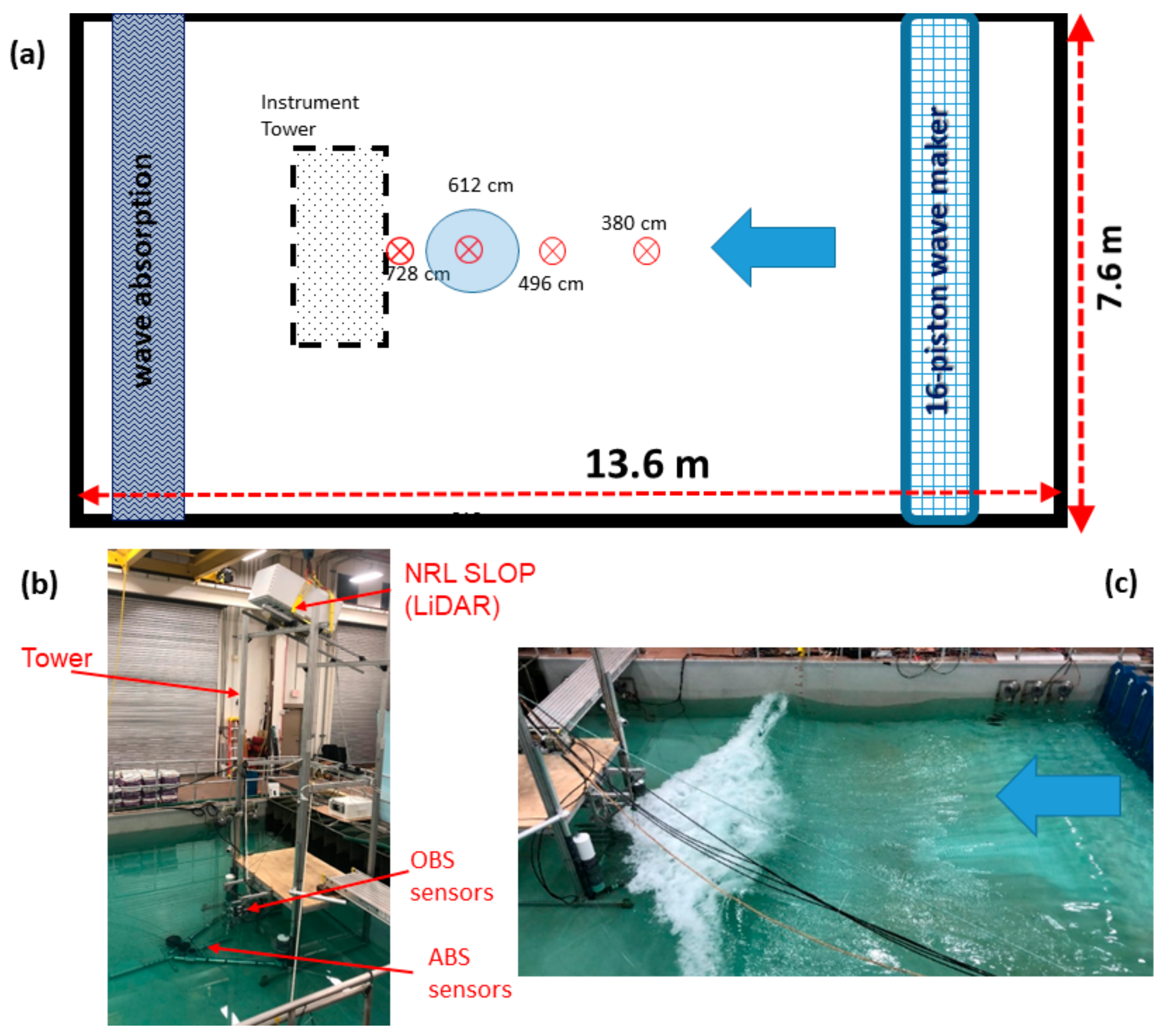
2.1. Wave Tank and Breaking Wave Generation

The experiments were performed in a wave tank at the Laboratory for Autonomous System Research (LASR) at the Naval Research Laboratory (NRL) in Washington, DC, USA. The LASR wave tank is a concrete pool 1.5 m deep, 13.7 m long (x-direction), and 7.6 m wide (y-direction) (Figure 1a). It is equipped with a 16-piston fully programmable mechanical wave maker (manufactured by HR Wallingford, Wallingford, UK) on one end and with porous wave energy absorbing material on the opposing end. During this experiment, the water level was kept at 0.91 m depth and the water temperature was about 23 °C. The salinity was brought up to 31 psu by adding Instant Ocean mixture. The water was filtered daily and the room was kept dark whenever possible to limit the accumulation of surfactants.

To maximize the amount of wave energy released during a singular breaking event at a planned location within this small wave tank, breaking waves were generated by means of dispersive wave focusing [25], combined with directional wave focusing. To achieve concurrent wave energy focusing at the planned location, each of the wave maker’s 16 pistons were operated independently allowing for longer propagation from the side piston to the center of the tank, than from center pistons. The dispersive wave focusing method utilized by each piston generates a wide frequency band chirp signal, designed to focus the maximum amount of wave energy at a desired location in time and space. It also allows independent fine-tuning of the generated wave phase to ensure that the wave packet energy maximum at the targeted focal point coincides with a wave crest. This ensures the same focal time and location with different propagation distances for waves by each piston. This feature is particularly useful to correct for nonlinear effects (otherwise not accounted for), which tends to shift the energy peak of the wave packet at the focal point towards an earlier time.

This generates an energetic overturning breaking wave crest during the bubble generation phase (active wave breaking phase) followed by a long bubble plume decay phase (i.e., passive phase) (Figure 1c). The resulting wave packet was measured by an array of four resistance wave gauges positioned along the center line throughout the wave tank (Figure 1a). The first wave gauge is positioned at the targeted focal point at the along-tank distance of x = 380 cm to the wavemaker. The following three gauges were positioned at x = 496 cm, 612 cm and 728 cm further away from the wavemaker. The gauge at location x = 612 cm is within the LiDAR measurement footprint. The wave elevation measurements by the gauge at the target focal point mark the beginning of wave breaking with active breaking extending out to the third wave gauge and eventually passive plume reaching the last wave gauge. The overall size of the breaking waves extended approximately up to 3 m in the along-tank direction, approximately the same in the cross-tank direction, and nearly all the way to the bottom in vertical direction (Figure 1c).

2.2. Breaking-Wave Bubble Mesurements Setup

An instrument tower was built and installed inside the tank for mounting underwater optical backscatter (OBS) and acoustic backscatter (ABS) sensors and an above-water LiDAR system (Figure 1b). The tower was constructed out of 80/20 aluminum alloy with a 1.8 m × 1.8 m surface footprint reaching up to 6.1 m up above the bottom of the wave tank. Backscatter measurements of breaking wave bubbles were taken continuously from the collocated OBS, ABS, and LiDAR sensor systems during the repeated wave breaking generations.

2.2.1. In-Water OBS and ABS Measurement Systems

Two submersible OBS systems were installed in a vertical array to measure breaking wave bubbles in this experiment. The first was the ECO Pucks (Sea-Bird Scientific, Bellevue, WA, USA) consisting of two OBS (90° incidence angle) sensors operating at 530 nm and 650 nm wavelengths, both flashing and collecting measurements at 10 Hz sampling rate. Three ECO Pucks were positioned at 4 cm, 20 cm, and 36 cm depths below the tank water surface. The second was the OBS-3+ (Campbell Scientific, Logan, UT, USA), measuring at 850 nm wavelength. Four OBS-3+ sensors were positioned at depths of 15 cm, 32 cm, 48 cm, and 64 cm to collect turbidity measurements at 100 Hz sampling rate. These OBS-3+ sensors are less sensitive to bubbles than the ECO Puck. However, they were added to the vertical array to supplement the backscatter measurement. These additional measurements are especially useful during the first two seconds of the breaking wave (i.e., active phase), when ECO Pucks were often oversaturated and could not be relied upon.

Two multiple-frequency upward-looking autonomous echo sounders, Acoustic Zooplankton Fish Profilers (AZFP, ASL Environmental Sciences, Victoria, BC, Canada), were installed on the tank bottom for ABS profile measurements of bubbles (Figure 1b). The first AZFP operates at lower acoustic frequencies of 38 kHz, 125 kHz, 200 kHz, and 455 kHz and the second AZFP operates at higher acoustic frequencies of 455 kHz, 769 kHz, 1250 kHz and 2000 kHz. The profile of ABS volume backscattering strength, Sv (dB), was collected at 1 Hz with a 1.2 cm vertical resolution. The Sv profile data by the high-frequency AZFP (455 kHz, 769 kHz, and 2000 kHz) show stronger variations and are analyzed for the study. ABS profiles of 455 kHz, 1250 kHz, and 2000 kHz correspond to bubble resonant radius of 7 µm, 3 µm, and 2 µm, respectively.

2.2.2. Above-Water LiDAR System

The Naval Research Laboratory (NRL) Shipboard Lidar, is a one-of-a-kind science tool developed and built by the Naval Air Warfare Center Aircraft Division. It is designed for detecting and characterizing subsurface layers in the upper ocean while the ship is underway or fixed on a station [26]. The laser parameters of the LiDAR transmitter and receiver are shown in

Table 1. Parameters of the LiDAR transmitter.

Parameter	Values
Wavelength	532 nm
Pulse energy	1 mJ
Repetition rate	50 Hz
Beam divergence	12 mrad (after beam expander)

and

Table 2. Parameters of the LiDAR receiver.

Parameter	Values
Telescope diameter	5 cm (6 units)
Field of view	140 mrad
Digitizer sample rate	800 MHz
Vertical sampling spacing	0.14 m (underwater)

, respectively. A set of four detectors with filters measure the different polarization states of light that is scattered out of the water. The combination of range gating and linear depolarization are used to differentiate the particle layers in the ocean. In order to understand how the lidar signal relates to the other instruments, it is necessary to understand what they are measuring. The lidar signal in bubbles fall into the small-angle scattering regime. This means that the calculation of [6] that relates the LiDAR backscatter to the void fraction is valid as long as the appropriate corrections are implemented. These corrections concern the water background correction and attenuation and are not dependent on the bubble size distribution [27].

The OBS turbidity and ECO Pucks instrument have a scattering geometry different from the lidar and they integrate the signal over a larger time scale (10 and 100 Hz vs. 800 MHz for the lidar). Generally, without a fully accurate model of these instruments’ optical specifications, the instruments should receive a stronger signal from the largest bubbles because the forward peak is smaller and will tend to keep the scattering within the receiver field of view. The forward peak width is also proportional to the wavelength and, in general, the OBS signal should be dependent on both the void fraction and the size of the bubbles.

In this experiment, the LiDAR system was mounted on the top of the instrument tower (4.37 m above the still water line) aiming towards the water at an angle of approximately 18° (Figure 1b). The current from the photomultiplier tubes (PMTs) of the LiDAR is recorded as “digitizer counts” due to the analog to digital conversion process. Several corrective steps are applied to assure the quality of LiDAR backscatter data. They are: (1) Converting the waveforms to volts from digital counts; (2) Removing the electronic and light background and correcting from the receiving geometry; (3) Removing electronic artifacts based on laboratory calibration to mitigate the presence of voltage overshoot; and (4) Normalizing the signal to take into account the gain of the PMT and convert the signal to Watts and into backscatter units (m⁻¹·sr⁻¹). A feature detection algorithm runs and separates bubbles from non-bubble data. Additional corrections are made based on statistical properties (i.e., attenuation) of the bubbles and non-bubbles data. After all these corrections, the algorithm can derive the void fraction of the bubble cloud, the injection rate of bubbles, and the decay rate of diffused bubbles The processed LiDAR subsurface backscatter profile data at 4.68 cm vertical resolution were collected at 50 Hz. More details of the LiDAR system calibration and data processing can be founded in [27].

3. Results and Discussion

The temporal variations of breaking-wave surfaces are tracked by elevation measurements from the four wave gauges. Samples of time series of wave elevations collected at the four locations are shown in Figure 2. The reference time for all four gauges starts at the time the wave crest is at the focal point (x = 380 cm). The crest-to-trough wave height $H_b$ and crest-to-crest wave period $T_w$ at the focal point are approximately estimated as 47 cm and 1.8 s, respectively. The crest-to-trough wave height decreases to 23 cm at the footprint of LiDAR. The local steepness ak at the focal point is 0.39, where amplitude a = 0.27 m, and wavenumber k = 1.44 m⁻¹ determined for $T_w$ = 1.8 s at tank water depth of 0.91 m by the linear wave dispersion relation. This steepness is within the steepness range reported by [28].

At the onset of wave breaking, injected bubbles are initially packed into high-concentration bubble plumes then disperse and dissipate into lower concentration through the processes of dissolution, diffusion, and degassing. Ultimately, entrained bubbles disappeared into the diffused background of low concentrations [29]. The evolution cycle of bubble plumes is depicted by intensity variations of LiDAR backscatter profiles. Figure 3a shows a 400-s segment of LiDAR backscatter profile measurements over three repeated wave breaking generations. The evolution cycle of backscatter intensification and decay is consistently reproduced in depth and time during the repeated wave breaking generations. This consistency enables the use of ensemble-averaged backscatter profile data from repeated breaking wave events for the study. The return from the tank bottom is not relevant to this study so only backscatter profile data above it were used in these analyses. The reference time of each breaking wave generation was determined as the breaking-wave elapsed time ($t_b$) from the first significant increase of near-surface LiDAR backscatter over background noise.

Based on the empirically estimated reference time for each breaking wave generation, ensemble-averaged LiDAR backscatter profiles $\beta \left(z,t_b\right)$ were obtained from 18 repeated individual breaking wave events (Figure 3b). Time history of LiDAR backscatter at depths of 7 cm, 17.5 cm and 31.5 cm was extracted from $\beta \left(t_b,z\right)$ (Figure 3c). Most significant variations of LiDAR backscatter occurred within the first few seconds ($t_b$ < 4 s). The LiDAR backscatter initially increases by two orders of magnitude over the background level (~10⁻⁴ Watts to 10⁻² Watts). The intensified backscatter then gradually decreases to ~5 × 10⁻³ Watts at $t_b$ = ~4 s. The backscatter in the upper 20 cm layer decreases very slowly to around ~3 × 10⁻⁴ Watts at $t_b$ = 20 s.

The temporal and spatial evolution in LiDAR backscatter profile data were compared against collocated OBS data collected at depths of 20.3 cm and 36.2 cm by the ECO Pucks (Figure 4). All LiDAR and OBS data were normalized by their peak backscatters. The rate of rapid intensification of LiDAR backscatter data shows some level of similarities to that of OBS data. In the decaying stage, LiDAR backscatter decreases faster than that of OBS data after $t_b$ = 3 s. Figure 5 shows comparisons of LiDAR data and OBS turbidity data (OBS-3+ at 850 nm) at depths of 12.1 cm and 31.8 cm. Both LiDAR and OBS data show a very rapid increase and decrease within $t_b$ < 2 s. After that, the decaying rate of LiDAR backscatter is slower than OBS turbidity of 850 nm.

Figure 4 implies that the void fraction decreases fast, with peaks at different relative intensity. The ECO puck temporal resolution shown here is relatively coarse and probably hides some of the detected variability. The difference between the LiDAR and ECO puck is consistent with the number of the largest bubbles decreasing faster at 20.3 cm depth than at 36.2 cm depth. Considering the overall decrease in void fraction, a higher number of small bubbles would be generated as a function of time as the larger bubbles outgas their content and their sizes decrease. At 20.3 cm depth, the larger relative increase of scattering at 650 nm is consistent with the larger forward peak at this wavelength. At 36.2 cm depth, the trend is different and both wavelengths behave the same. This could imply that overall, the ratio of the different bubble sizes is more stable at this depth. Considering Figure 5, the quick decrease of turbidity at 12.1 cm depth and the bi-modal distribution at 31.8 cm depth would be consistent with the turbidity sensor sensitive to a specific part of the bubble size distribution. This range of size would decrease quite fast at the surface but show a relative increase at the depth of 31.8 cm, even if the total void fraction decreases.

The temporal variations of LiDAR backscatter were compared against ABS data from the AZFP at depths of 10 cm and 31 cm (Figure 6). Both LiDAR and ABS backscatter data of 455 kHz, 1250 kHz, and 2000 kHz show a similar rapid intensification within the first few seconds of elapsed time when bubble concentration is expected to be high. However, when bubble plumes are dissipated into a lower concentration, the resulting decay of LiDAR backscatter intensity agrees better with the ABS data of 2000 kHz than ABS data of lower frequencies (455 kHz and 1250 kHz). These differences are related to the fact that the main contribution of the acoustic backscatter come from coherent return of a specific bubble size. It looks like the population of the smallest bubbles with a radius around 2 µm (ABS of 2000 kHz) follow the decrease of void fraction well. The above LiDAR backscatter comparisons against OBS and ABS at multiple wavelengths and wave frequencies show that LiDAR backscatter measurements of high-concentration bubble plumes during a wave breaking event are consistent with simultaneous changes of the void fraction and the size distribution. In the diffusive phase of breaking wave bubbles, the LiDAR backscatter of low-concentration dissipated bubble plumes is more similar to OBS of 850 nm and ABS of 2000 kHz. It would be interesting to know if similar results could be expected in natural breaking wave conditions.

The evolution scales of breaking-wave bubble plumes are related to breaking wave properties (wave height, $H_w$, and period, $T_w$). Void fraction measurements of breaking-wave bubble [30] showed high values of void fraction (80–99%) within a very short time period up to 0.25$T_w$ and the void fraction decreased to about 20% at 0.7$T_w$. The bubble plume depths can reach 0.5$H_w$ to 2$H_w$. Normalized LiDAR backscatter profile data $\beta /{\beta }_{max}$ are examined with time and depth scaled by wave period ($t_b/T_w$) and wave height ($z/H_w$), respectively (Figure 7). Most of the backscatter intensification is from high-concentration bubble plumes occurring during the active breaking phase ($t_b/T_w$ < 1.5). The contour line of $\beta /{\beta }_{max}=0.25$ depicts the depth evolution of high-concentration bubble plumes of active wave breaking. The maximum backscatter occurred at $t_b/T_w$ ~0.1 at depth $z/H_w$ ~0.1 followed by secondary peaks at $t_b/T_w$ ~1.2 and 2. The presence and periodicity of secondary peaks are likely caused by relatively lower concentration bubble plumes rising to the surface driven by the residual wave orbital motions following wave breaking [31,32]. After the active breaking, the LiDAR backscatter of dissipated bubbles decreases significantly. The depth of dissipated bubble plumes was approximated by contour line of $\beta /{\beta }_{max}=0.1$. The decaying backscatter from dissipated bubble plumes could last about three wave periods. There is a shallow layer of very low backscatter (0.2$H_w$) persisting for up to 5$T_w$.

Cox and Shin [33] found that the depth-averaged void fractions increase rapidly and linearly and then decay slowly and exponentially. Lamarre and Melville [34] and Rojas and Loewen [35] show the void fraction decaying rate by a power-law approximation ${\left(t_b/T_w\right)}^c$, where c has values of −2.3 and −2.6, respectively. The temporally varying characteristics of LiDAR bubble measurements were further examined based on depth-averaged backscatter $\langle \beta \rangle$ of near-surface layer ($z$ < 0.5$H_w)$ (Figure 7b). The normalized $\langle \beta \rangle /{\langle \beta \rangle }_{max}$ show major peaks at $t_b/T_w$= 0.1 and then at $t_b/T_w$ = 1.2 with 50% of peak values. The decaying rate of backscatter of dissipated bubbles at $t_b/T_w$ > 2 is approximated by a power law as $\langle \beta \rangle /{\langle \beta \rangle }_{max}~{\left(t_b/T_w\right)}^c$, where c = −3.3. Assuming the linear proportionality between LiDAR backscatter and void fraction [6], the decaying rate of $\langle \beta \rangle /{\langle \beta \rangle }_{max}$ is qualitatively comparable with variations in void fraction measurements of bubble plumes in previous studies [32,33].

4. Conclusions

Laboratory experiments were conducted to evaluate the feasibility of profiling and characterizing breaking-wave bubble plumes from an above-water Light Detection and Ranging (LiDAR) system. We deployed the NRL in-house LiDAR system to conduct LiDAR backscatter profile measurements of bubble plumes under mechanically generated plunging breakers in a wave tank. The temporal variations of LiDAR backscatter are compared against collocated measurements by in-water optical and acoustic backscatter (OBS and ABS) sensors. The variations of LiDAR backscatter follow well the population of small size bubbles, similar to the variations of ABS data at 2000 kHz and also show interesting similarities with the OBS data at 850 nm, even if the reason is probably more complex.

The variation characteristics of rapid intensification and decay in LiDAR backscatter data of bubble plumes scaled by surface wave height and period are consistent with studies based on void fraction measurements of bubbles. More validation experiments of LiDAR backscatter measurements under a wider range of breaking wave conditions should be planned. Collocated void fraction and bubble distribution measurements should be conducted and analyzed to validate the linear proportionality between LiDAR backscatter and void fraction of bubble plumes.

This proof-of-concept study demonstrates the viability of deploying an above-water LiDAR system to remotely profile subsurface breaking wave bubble plumes and eventually determine the total volume of entrained air by breaking waves in the open ocean. This could pave the way to eventually develop an airborne LiDAR operation for global coverage of subsurface bubble plumes.

References

1. Thorpe, S.A. On the clouds of bubbles formed by breaking wind-waves in deep water, and their role in air-sea gas transfer. Philos. Trans. R. Soc. London. Ser. A Math. Phys. Sci. 1982, 304, 155–210. [Google Scholar] [CrossRef]
2. Deane, G.B.; Stokes, M.D. Model calculations of the underwater noise of breaking waves and comparison with experiment. J. Acoust. Soc. Am. 2010, 127, 3394–3410. [Google Scholar] [CrossRef] [PubMed]
3. Longuet-Higgins, M.S.; Turner, J.S. An ‘entraining plume’ model of a spilling breaker. J. Fluid Mech. 1974, 63, 1–20. [Google Scholar] [CrossRef]
4. Banner, M.L.; Cato, D.H. Physical mechanisms of noise generation by breaking waves—A laboratory study. In Sea Surface Sound; Springer: Dordrecht, The Netherlands, 1988; pp. 429–436. [Google Scholar]
5. Lamarre, E.; Melville, W.K. Void-fraction measurements and sound-speed fields in bubble plumes generated by breaking waves. J. Acoust. Soc. Am. 1994, 95, 1317–1328. [Google Scholar] [CrossRef]
6. Churnside, J.H. Lidar signature from bubbles in the sea. Opt. Express 2010, 18, 8294–8299. [Google Scholar] [CrossRef]
7. Cipriano, R.J.; Blanchard, D.C. Bubble and aerosol spectra produced by a laboratory ‘breaking wave’. J. Geophys. Res. Earth Surf. 1981, 86, 8085–8092. [Google Scholar] [CrossRef]
8. Medwin, H.; Daniel, A.C. Acoustical measurements of bubble production by spilling breakers. J. Acoust. Soc. Am. 1990, 88, 408–412. [Google Scholar] [CrossRef]
9. Loewen, M.R.; O’Dor, M.A.; Skafel, M.G. Bubbles entrained by mechanically generated breaking waves. J. Geophys. Res. Earth Surf. 1996, 101, 20759–20769. [Google Scholar] [CrossRef]
10. Leifer, I.; De Leeuw, G.; Cohen, L.H. Optical Measurement of Bubbles: System Design and Application. J. Atmos. Ocean. Technol. 2003, 20, 1317–1332. [Google Scholar] [CrossRef] [Green Version]
11. Medwin, H. In situ acoustic measurements of bubble populations in coastal ocean waters. J. Geophys. Res. Earth Surf. 1970, 75, 599–611. [Google Scholar] [CrossRef]
12. Vagle, S.; Farmer, D.M. The Measurement of Bubble-Size Distributions by Acoustical Backscatter. J. Atmos. Ocean. Technol. 1992, 9, 630–644. [Google Scholar] [CrossRef]
13. Wang, D.W.; Wijesekera, H.W.; Jarosz, E.; Teague, W.J.; Pegau, W.S. Turbulent Diffusivity under High Winds from Acoustic Measurements of Bubbles. J. Phys. Oceanogr. 2016, 46, 1593–1613. [Google Scholar] [CrossRef]
14. Strand, K.O.; Breivik, Ø.; Pedersen, G.; Vikebø, F.B.; Sundby, S.; Christensen, K.H. Long-Term Statistics of Observed Bubble Depth Versus Modeled Wave Dissipation. J. Geophys. Res. Oceans 2020, 125, e2019JC015906. [Google Scholar] [CrossRef]
15. Josset, D.B.; Wang, D.W.; Savelyev, I.; Anguelova, M.D.; Keiffer, R.S.; Fabre, J.P. On the retrieval of bubble properties from space lidar and their impact on acoustic transmission loss. In Ocean Sciences Meeting; AGU: San Diego, CA, USA, 2020. [Google Scholar]
16. Salisbury, D.J.; Anguelova, M.D.; Brooks, I.M. On the variability of whitecap fraction using satellite-based observations. J. Geophys. Res. Oceans 2013, 118, 6201–6222. [Google Scholar] [CrossRef] [Green Version]
17. Anguelova, M.D.; Bettenhausen, M.H. Whitecap Fraction from Satellite Measurements: Algorithm Description. J. Geophys. Res. Oceans 2019, 124, 1827–1857. [Google Scholar] [CrossRef]
18. Burrage, D.M.; Anguelova, M.D.; Wang, D.W.; Wesson, J.C. Predicting radiometric effects of a Rough Sea surface, whitecaps, foam, and spray using SURFER 2D. IEEE J. Sel. Top. Appl. Earth Obs. Remote Sens. 2019, 12, 3194–3207. [Google Scholar] [CrossRef]
19. Anguelova, M.D.; Gaiser, P.W. Skin depth at microwave frequencies of sea foam layers with vertical profile of void fraction. J. Geophys. Res. Earth Surf. 2011, 116, C11002. [Google Scholar] [CrossRef] [Green Version]
20. Churnside, J.H. Review of profiling oceanographic lidar. Opt. Eng. 2013, 53, 051405. [Google Scholar] [CrossRef] [Green Version]
21. Chen, P.; Pan, D. Ocean Optical Profiling in South China Sea Using Airborne LiDAR. Remote Sens. 2019, 11, 1826. [Google Scholar] [CrossRef] [Green Version]
22. Krekova, M.M.; Krekov, G.M.; Shamanaev, V.S. Influence of Air Bubbles in Seawater on the Formation of Lidar Returns. J. Atmos. Ocean. Technol. 2004, 21, 819–824. [Google Scholar] [CrossRef]
23. Li, W.; Yang, K.; Xia, M.; Rao, J.; Zhang, W. Influence of characteristics of micro-bubble clouds on backscatter lidar signal. Opt. Express 2009, 17, 17772–17783. [Google Scholar] [CrossRef] [PubMed]
24. Liu, Q.; Liu, D.; Bai, J.; Liu, N.; Zhang, Y.; Shen, X. Influence of ocean surface waves and air bubbles on the polarization characteristics of spaceborne oceanographic lidar returns. In Remote Sensing of the Ocean, Sea Ice, Coastal Waters, and Large Water Regions; International Society for Optics and Photonics: Bellingham, WA, USA, 2018; Volume 10784, p. 107840O. [Google Scholar] [CrossRef]
25. Handler, R.A.; Savelyev, I.; Lindsey, M. Infrared imagery of streak formation in a breaking wave. Phys. Fluids 2012, 24, 121701. [Google Scholar] [CrossRef]
26. Gould, R.; Josset, D.; Anderson, S.; Goode, W. Estimating Oil Slick Thickness with LiDAR Remoter Sensing Technology; Final Report; Bureau of Safety and Environmental Enforcement (BSEE): Washington, DC, USA, 2019.
27. Josset, D.; Cayula, S.; Concannon, B.; Sova, S.; Weidemann, A. On the bubble-bubbleless ocean continuum: Lidar measurement of underwater bubble properties during storm conditions. J. Atmos. Ocean. Technol. 2022, unpublished work. [Google Scholar]
28. Rapp, R.J.; Melville, W.K. Laboratory measurements of deep-water breaking waves. Philosophical Transactions of the Royal Society of London. Ser. A Math. Phys. Sci. 1990, 331, 735–800. [Google Scholar]
29. Deane, G.B.; Stokes, M.D. Air Entrainment Processes and Bubble Size Distributions in the Surf Zone. J. Phys. Oceanogr. 1999, 29, 1393–1403. [Google Scholar] [CrossRef]
30. Anguelova, M.D.; Huq, P. Characteristics of bubble clouds at various wind speeds. J. Geophys. Res. Earth Surf. 2012, 117, C03036. [Google Scholar] [CrossRef] [Green Version]
31. Leifer, I.; De Leeuw, G. Bubbles generated from wind-steepened breaking waves: 1. Bubble plume bubbles. J. Geophys. Res. Ocean. 2006, 111, C06020. [Google Scholar] [CrossRef] [Green Version]
32. Deike, L.; Melville, W.K.; Popinet, S. Air entrainment and bubble statistics in breaking waves. J. Fluid Mech. 2016, 801, 91–129. [Google Scholar] [CrossRef] [Green Version]
33. Cox, D.T.; Shin, S. Laboratory Measurements of Void Fraction and Turbulence in the Bore Region of Surf Zone Waves. J. Eng. Mech. 2003, 129, 1197–1205. [Google Scholar] [CrossRef]
34. Lamarre, E.; Melville, W.K. Air entrainment and dissipation in breaking waves. Nature 1991, 351, 469–472. [Google Scholar] [CrossRef]
35. Rojas, G.; Loewen, M.R. Void fraction measurements beneath plunging and spilling breaking waves. J. Geophys. Res. Earth Surf. 2010, 115, C08001. [Google Scholar] [CrossRef]
Figure 1. (a) Sketch of LASR wave tank and experiment setup; (b) Instrument tower and installed measurement sensors; (c) A snap shot of wave breaking. The red circled crosses in (a) mark the wave gauge locations (x = 380 cm, 496 cm, 612 cm, and 728 cm). The blue shaded circle in (a) is the footprint location of LiDAR. The arrows in (a,c) are the wave propagation direction.
Remotesensing 14 01680 g001
Figure 2. Time series of wave elevation measured at four locations along the center line of the tank.
Remotesensing 14 01680 g002
Figure 3. (a) Samples of subsurface profile measurements of LiDAR backscatter intensity (Watts) during three repeated breaking-wave generations. (b) Ensemble-averaged LiDAR backscatter vertical profiles. Colorized backscatter intensity (Watts) is on a logarithmic scale of base 10. (c) Time series of ensemble-averaged LiDAR backscatter intensity at depths of 7 cm, 17.5 cm, and 31.5 cm.
Remotesensing 14 01680 g003
Figure 4. Time series of normalized backscatter of LiDAR and ECO Puck OBS sensors at depths of (a) 20.3 cm and (b) 36.2 cm.
Remotesensing 14 01680 g004
Figure 5. Time series of normalized backscatter intensity of LiDAR and OBS turbidity at depths of (a) 12.1 cm and (b) 31.8 cm. The sampling rate of turbidity is 100 Hz.
Remotesensing 14 01680 g005
Figure 6. Time evolution of normalized backscatter of LiDAR and ABS data of 455 kHz, 1250 kHz and 2000 kHz at depths (a) 10 cm and (b) 31 cm.
Remotesensing 14 01680 g006
Figure 7. (a) Time-depth plot of ensemble-averaged profiles normalized by the peak value, β / β m a x . Elapsed time ( t b ) and depth ( z ) are normalized by wave period ( T w ) and breaking wave height ( H w ), respectively. The gray dotted and dashed lines represent the contour lines of β / β m a x of 0.25 and 0.1, respectively. (b) Near-surface depth-averaged LiDAR intensity β normalized by the maximum mean intensity of the breaking event. The dashed line represents a power-law decaying, β / β m a x ~ a t b / T w c , where a = 2 and c = −3.3.
Remotesensing 14 01680 g007