Communication

Generating High-Resolution and Long-Term SPEI Dataset over Southwest China through Downscaling EEAD Product by Machine Learning

1
Faculty of Geosciences and Environmental Engineering, Southwest Jiaotong University, Chengdu 610031, China
2
Key Laboratory for Geographical Process Analysis & Simulation of Hubei Province/School of Urban and Environmental Sciences, Central China Normal University, Wuhan 430079, China
3
Macro Agriculture Research Institute, College of Resources and Environment, Huazhong Agricultural University, Wuhan 430070, China
*
Author to whom correspondence should be addressed.
Remote Sens. 2022, 14(7), 1662; https://doi.org/10.3390/rs14071662
Submission received: 17 February 2022 / Revised: 22 March 2022 / Accepted: 28 March 2022 / Published: 30 March 2022

Abstract

:
Drought is an event of shortages in the water supply, whether atmospheric, surface water or ground water. Prolonged droughts have negative impacts on ecosystems, agriculture, society, and the economy. Although existing drought index products are widely utilized in drought monitoring, the coarse spatial resolution greatly limits their applications on regional or local scales. Machine learning driven by remote sensing observations offers an opportunity to monitor regional scale droughts. However, the limited time range of remote sensing observations such as vegetation index (VI) resulted in a substantial gap in generating high resolution drought index products before 2000. This study generated spatiotemporally continuous Standardized Precipitation Evapotranspiration Index (SPEI) data spanning from 1901–2018 in southwestern China by machine learning. It indicated that four Classification and Regression Tree (CART) approaches, decision trees (DT), random forest (RF), gradient boosted regression trees (GBRT) and extra trees (ET), can provide valid local drought information by downscaling the Estación Experimental de Aula Dei (EEAD) data. The in-situ SPEI dataset produced by the Penman–Monteith method was used as a benchmark to evaluate the temporal and spatial performance of the downscaled SPEI. In addition, the necessity of VI in SPEI downscaling was also assessed. The results showed that: (1) the ET-based product has the best performance (R2 = 0.889, MAE = 0.232, RMSE = 0.432); (2) the VI provides no significant improvement for SPEI re-construction; (3) topography exerts an obvious influence on the downscaling process, and (4) the downscaled SPEI shows more consistency with the in-situ SPEI compared with EEAD SPEI. The proposed method can be easily extended to other areas without in-situ data and enhance the ability of long-term drought monitoring.

1. Introduction

Drought, as one of the major natural disasters in the world, is costly; it causes huge harm to agriculture, the environment, and the social economy each year [1,2,3,4]. Economic stress and disruption caused by natural disasters are escalating at an alarming rate, which calls for forward-looking risk management [5]. Drought monitoring and prediction can help policy makers’ response to drought events [6,7]. Therefore, persistent drought monitoring and prediction are critical to decision-making processes for the sustainable management of water resources and drought risk management [8,9,10].
Drought is an event of shortages in the water supply, whether atmospheric, surface water or ground water [11]. Earlier studies monitored drought generally with univariate indices, which characterize only one component in the water balance, e.g., Standardized Precipitation Index (SPI) [12], Standardized Runoff Index (SRI) [13], and Standardized Soil Moisture Index (SSMI) [14]. These univariate indices could not fully represent a drought event [15,16,17]. Thus, several multivariate drought indices were proposed, including the Palmer Drought Severity Index (PDSI) [18] and Standardized Precipitation Evapotranspiration Index (SPEI) [19]. In contrast to the PDSI, the SPEI can be obtained at varying time scales, which is crucial to representing the lagged and cumulative effects of drought [20,21]. Specifically, the 3-month scale SPEI has been widely used in monitoring and assessing agriculture drought [22,23,24], as it can satisfactorily capture the vegetation response to drought [25,26]. Recently, researchers have derived a drought index based on reanalysis data, such as the Estación Experimental de Aula Dei (EEAD) SPEI and the Climatic Research Unit (CRU) self-calibrating PDSI. These products mentioned above are characterized by low spatial resolution (0.5° spatial resolution), but elaborate drought monitoring in small areas requires high-resolution data.
In recent years, machine learning methods, e.g., cubist, random forest (RF), boosted regression trees and gradient boosted regression trees (GBRT), have been widely used to obtain a high-resolution product [27,28,29], however, their performances vary significantly depending on the target variable and the training dataset [30,31]. Previous studies mainly constructed a relationship model between the in-situ drought index and other variables by using machine learning [29,32,33,34,35]. Another approach is to aggregate the surface variables into a low-resolution grid and build a relationship model between the surface variables and low-resolution target variable [36,37]. Large numbers of studies have demonstrated the potential of the vegetation index (VI) in characterizing drought [32,38,39,40].
Previous studies are more focused on using the remote sensing datasets such as VI as input variables, resulting in a substantial gap in high resolution drought index products before 2000. It is impossible to collect VIs at the early time before the satellite launch, limiting the temporal coverage of these methods. For example, the Moderate Resolution Imaging Spectroradiometer (MODIS) VI data are available only for the period after 2000 [32,41]. Since VI is not an independent variable, other parameters (such as temperature and precipitation) may contain enough information to represent VI [42,43].
Therefore, as an extension of the previous studies, we focused on generating high-resolution drought indices before 2000. The overall objective of this study is to identify the necessity of VI in downscaling the SPEI and generate a 1 km and long-term (1901–2018) SPEI dataset to investigate the local elaborate drought. Specific objectives include: (1) comparing four commonly used machine learning methods in drought indicator downscaling, including decision trees (DT), RF, GBRT, and extra trees (ET); (2) identifying the necessity of VI in downscaling the SPEI; (3) downscaling the EEAD product to generate a long-term (1901 through 2018), 1 km, and monthly SPEI dataset with a 3-month temporal scale; and finally, (4) validating the generated dataset. Our study was implemented over Southwest China, where is located the largest terrestrial carbon sink in China, and which is prone to severe drought.

2. Materials and Methods

2.1. Study Area

The study area is situated in Southwest China, composed of four provinces and a municipality, including Sichuan, Yunnan, Guizhou, Guangxi, and Chongqing municipality (Figure 1). The climate is dominated by a subtropical monsoon climate with warm, wet summers, causing a high vegetation coverage [44,45]. Our study area is the largest carbon reservoir of China, accounting for more than 30% of CO2 uptake in Chinese mainland [46,47]. However, Southwestern China has the large area of karst landform, with fragile ecosystems and frequent clouds, making plant growth in the region vulnerable to drought.
Over the past 30 years, the growing population has increased the demand for water in Southwest China, and drought has become a repeatedly natural disaster in this area, causing great agricultural loss and severe drinking water shortage. For example, the 2009 drought reportedly resulted in declined vegetation productivity and drink water shortage for 8.1 million people [48]. Drought, in 2011, caused the destruction of more than 98.9 million hectares of crops and the lack of drinking water for more than 4.9 million people [49].

2.2. Data

Several streams of data were involved in our study (see Table 1). In-situ climate data, including precipitation, temperature, wind speed, and sunshine duration, over 145 meteorological stations spanning 1961 through 2015, were downloaded from the National Tibetan Plateau Scientific Data Center (TPDC) (Figure 1). They were applied to calculate the in-situ SPEI to evaluate the downscaled dataset. The potential evapotranspiration in the in-situ SPEI is from the Penman–Monteith method to match the EEAD SPEI [50]. The 1 km and monthly gridded climate dataset (GCD) including precipitation and temperature data spanning 1901 through 2018 were also downloaded from the TPDC. They are important independent variables to construct the relationship model to estimate the SPEI. This dataset was generated from CRU v4.02 and WorldClim datasets by Delta downscaling method [51]. The daily MCD43A4 data was used to obtain VI data including the Normalized Difference Vegetation Index (NDVI) and Enhanced Vegetation Index (EVI) to identify the necessity of VI in downscaling the SPEI. NDVI information is more about spatial differences in vegetation and EVI focuses on expressing the seasonal change of vegetation. Substantial studies have demonstrated that when combined, they can better characterize the vegetation information [52]. The monthly 0.5° gridded SPEI from 1901 to 2018, downloaded from EEAD, is referred to as EEAD SPEI hereafter. This dataset was calculated based on the CRU dataset and the potential evapotranspiration in SPEI is from the Penman–Monteith method [50]. The Digital Elevation Model (DEM) collected from Resource and Environmental Science Data Platform of the Chinese Academy of Sciences was used to analyze the topographic dependence of the downscaled SPEI.

2.3. Methods

Figure 2 reveals the flowchart of the downscaling procedure in this study. The downscaling process includes three main steps: generation of the training dataset, method selection, and validation. Details are elaborated as follows:
Generation of training dataset: The NDVI, EVI, and the GCD precipitation and temperature both with 1-km resolution were first aggregated into the 0.5° grid by averaging all values within each grid to match the resolution of the EEAD SPEI data. There were a total of seven variables: NDVI, EVI, precipitation, temperature, latitude, month, and year were used as potential independent variables, and the EEAD SPEI were used as dependent variables. 20% of the samples were randomly selected and used for validation, and the remaining 80% were used as training data [53,54].
Method selection: Four tree-based machine learning approaches, DT, RF, GBRT and ET, were compared in terms of SPEI downscaling. A preliminary evaluation was performed to compare the accuracy of the regression results of the four approaches. A larger coefficient of determination (R2) value indicates better goodness-of-fit, and the perfect score of the R2 is 1. A lower Mean Absolute Error (MAE) and Root-Mean-Square Error (RMSE) value indicate higher accuracy, and the perfect score of MAE and RMSE is 0 [55,56]. R2, MAE and RMSE between the EEAD SPEI and the estimated SPEI at the EEAD grid scale were obtained and compared:
R 2 = 1 i = 1 N ( S P E I i e s t S P E I i o b s ) 2 / i = 1 N ( S P E I i e s t S P E I i o b s ¯ ) 2
R M S E = i = 1 N ( S P E I i e s t S P E I i o b s ) 2 N
M A E = i = 1 N | S P E I i e s t S P E I i o b s | N
where S P E I i e s t is the estimated SPEI value from machine learning and S P E I i o b s is the EEAD value.
During the method selection procedure, NDVI and EVI were not included in the training dataset, as they span a very limited temporal coverage (from 2000–2018) compared with other variables (1901–2018), which would reduce the representativeness of the results. For further identification of the necessity of VI in downscaling SPEI, two input combinations, with and without the two VIs, were used to drive the selected best model (ET). At this step, the model runs for the period of 2001–2018, concurrent with the MODIS acquisition time in this study. In addition to R2, RMSE and MAE, a t-test was also used to examine whether the two results have a significant difference. We propose that if there was no significant difference between the two combinations, the parsimony one without VIs would be preferred, as this combination would greatly extend the temporal coverage from 2000–2018 to 1901–2018.
Validation: The downscaled SPEI data was validated through direct comparison with the in-situ SPEI calculated from site-measured meteorological data by the SPEI R package (https://CRAN.R-project.org/package=SPEI (accessed on 12 February 2022)). An identical algorithm configuration was selected as that for the EEAD product to avoid uncertainty caused by different SPEI definitions. To match the temporal coverage of the downscaled SPEI data and in-situ SPEI, we used the standardized anomaly to obtain the number of standard deviations (SD) of SPEI from its multi-year average during the operational period of the selected meteorological stations (1961–2015). In addition, DEM was used to quantitatively analyze the topographic dependence of the accuracy.
According to SPEI classification, the drought events in this study were identified by a SPEI value less than −0.5 (the threshold = −0.5) for each month [23]. For each decade, we calculated three common drought metrics: duration, intensity, and frequency [57]. Duration was defined as the number of consecutive months for which SPEI was below the drought threshold. Frequency is the number of drought events over a decade. Intensity is the difference between the drought threshold and the monthly SPEI, averaged over all months during a drought event.
To show the potential of the downscaled SPEI in the characterization of high-resolution spatial-temporal dynamics of drought episodes, we compared the time series of the downscaled and the original EEAD SPEI data. Finally, the extreme drought events during 2009–2010 were selected to compare the spatial and temporal disparities between them.

3. Results

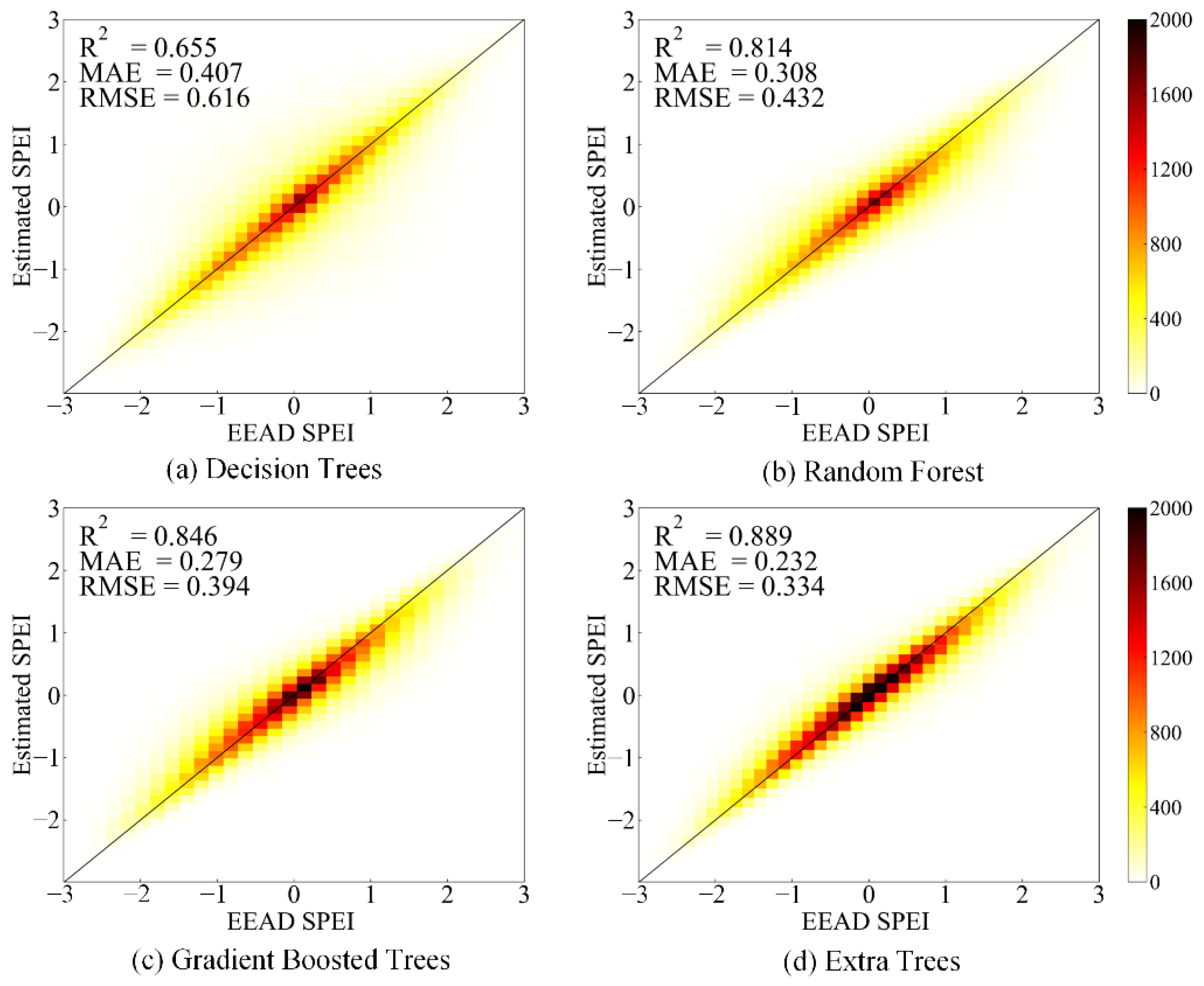
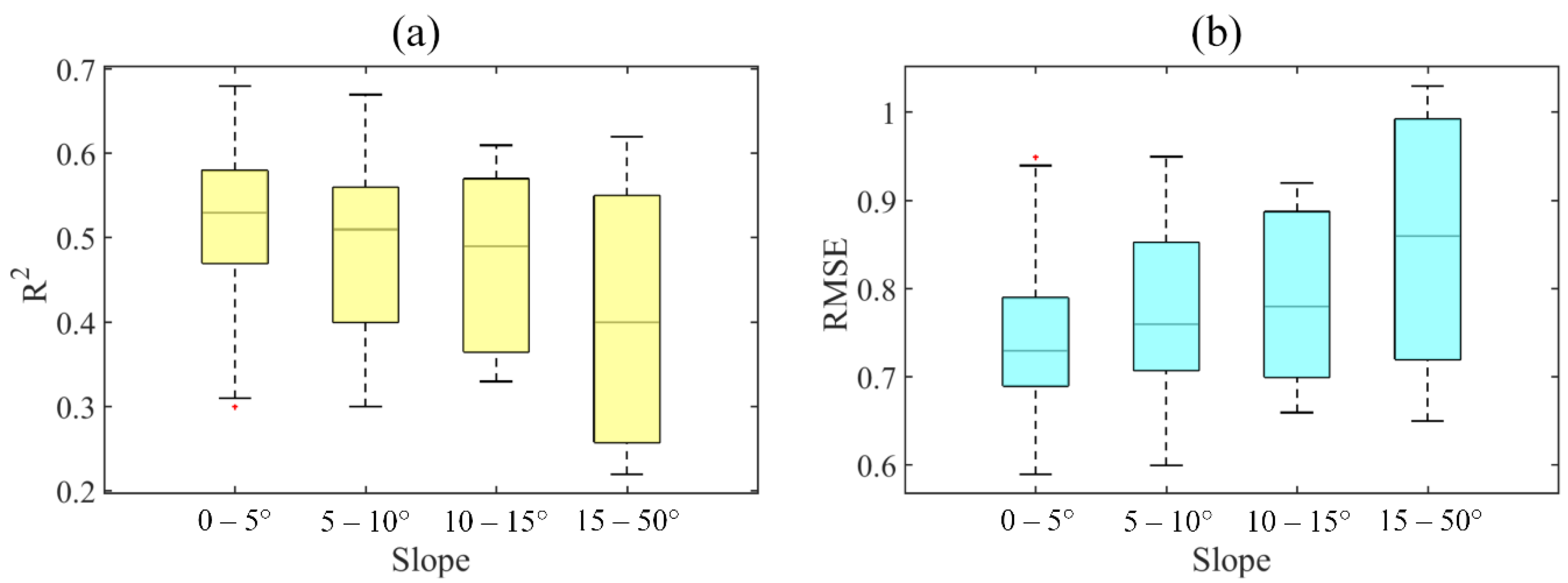
3.1. Method Comparison with Cross-Validation

Figure 3 shows the cross-validation results for predicted SPEI from different machine learning methods (DT RF, GBRT and ET), with the EEAD 3-month SPEI values in the test dataset as reference. The accuracy of single DT (DT: R2 = 0.655, RMSE = 0.616, MAE = 0.407; see Figure 3a) is much lower than the other three methods. Compared with Single DT, ET and RF fit a large number of random DTs on various subsamples of the dataset and average them to improve prediction accuracy [58]. A GBRT was built by combining several weak learners into one powerful ensemble. Weak learners are combined in turn, and each new model attempts to correct the prediction bias of all the previous models [29,59]. ET shows the best performance with R2 = 0.889, MAE = 0.232 and RMSE = 0.432. Therefore, ET was selected to downscale the EAAD SPEI products.

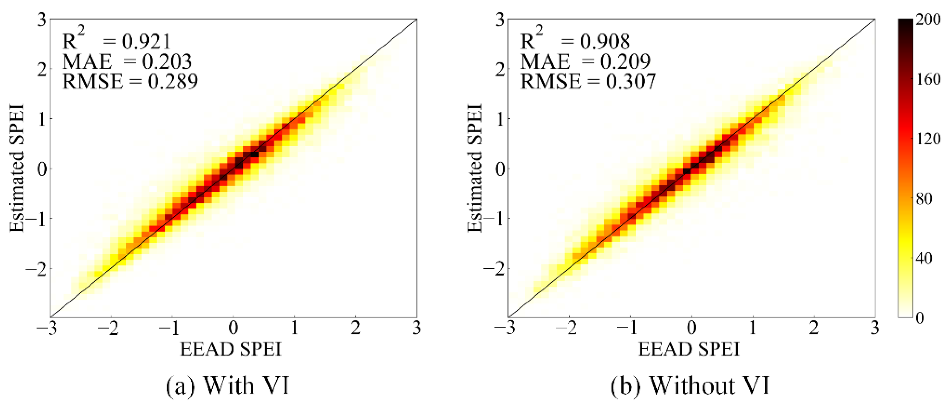
3.2. Influence of Vegetation Indices on Method Performance

Both input combinations with and without VI using the ET model were tested in our study (Figure 4). Their performances were comparable (R2: 0.921 vs. 0.908, MAE: 0.203 vs. 0.209, and RMSE: 0.289 vs. 0.307). A t-test revealed no significant difference between the two combinations (p < 0.01). VI has very limited temporal span. For example, MODIS VI cannot be obtained before 2000. Therefore, we did not use VI in our study, and this ensured the generation of a very long-term high spatial resolution SPEI, concurrent with the EEAD and GCD products (1901 through 2018).

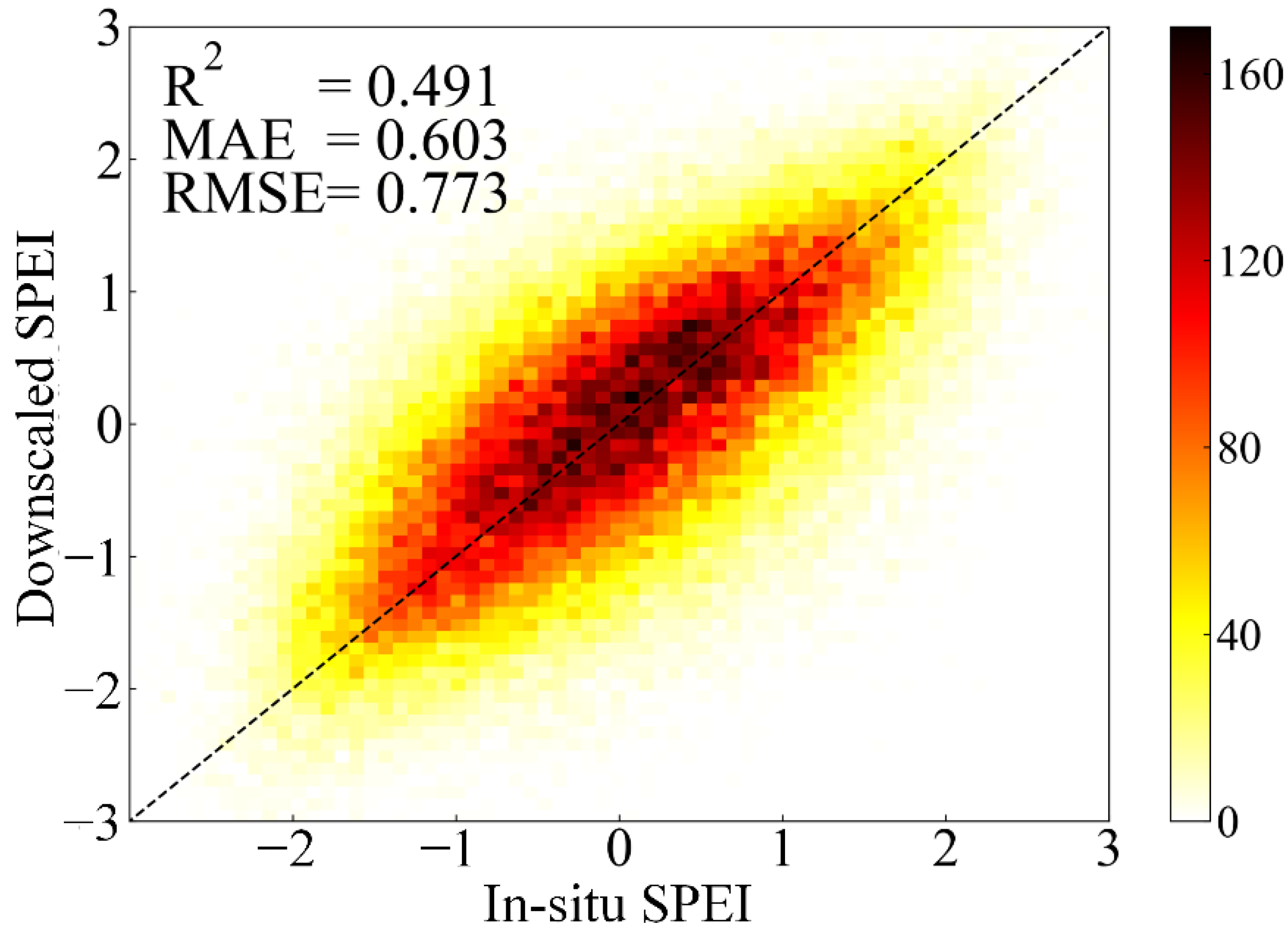
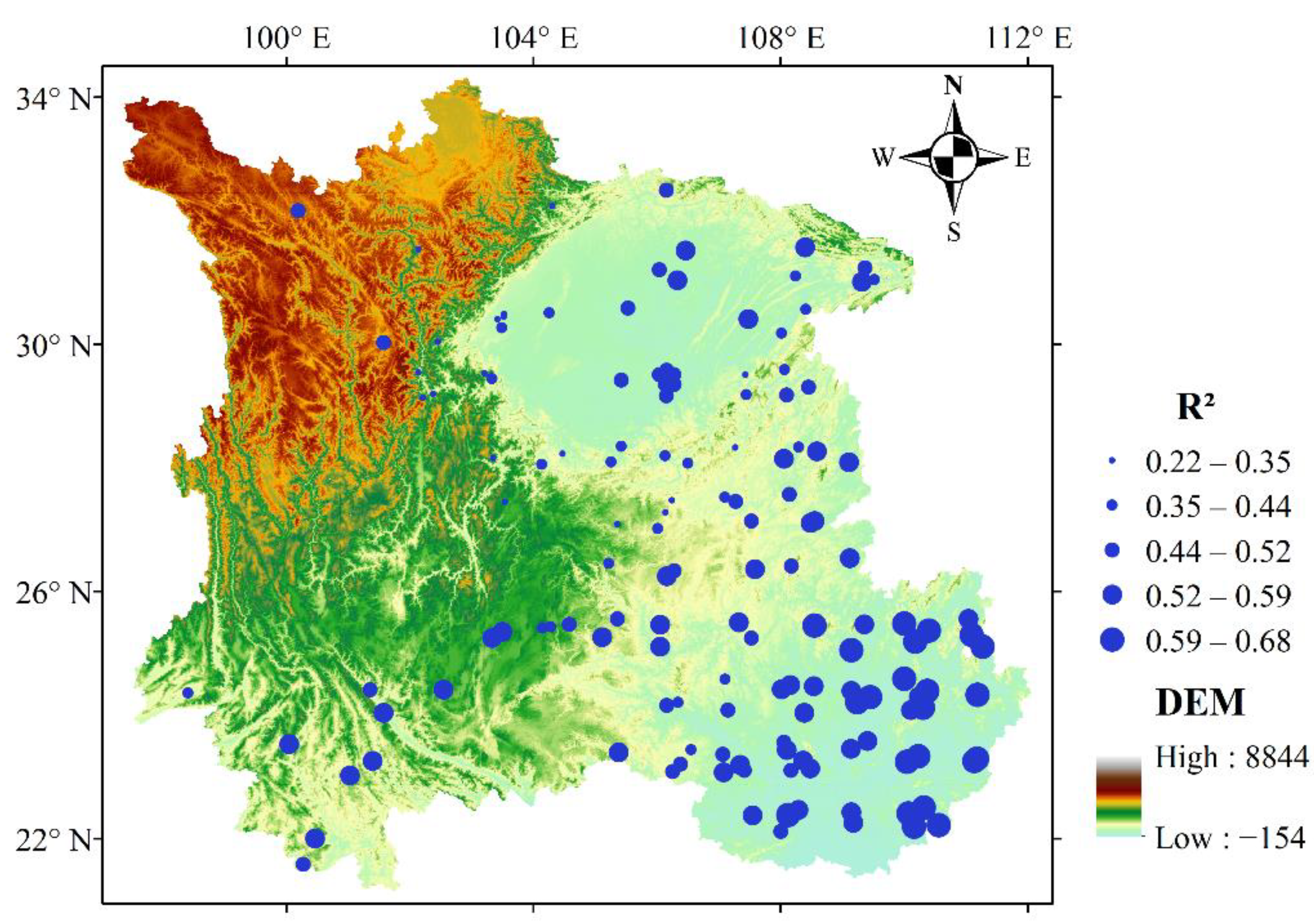
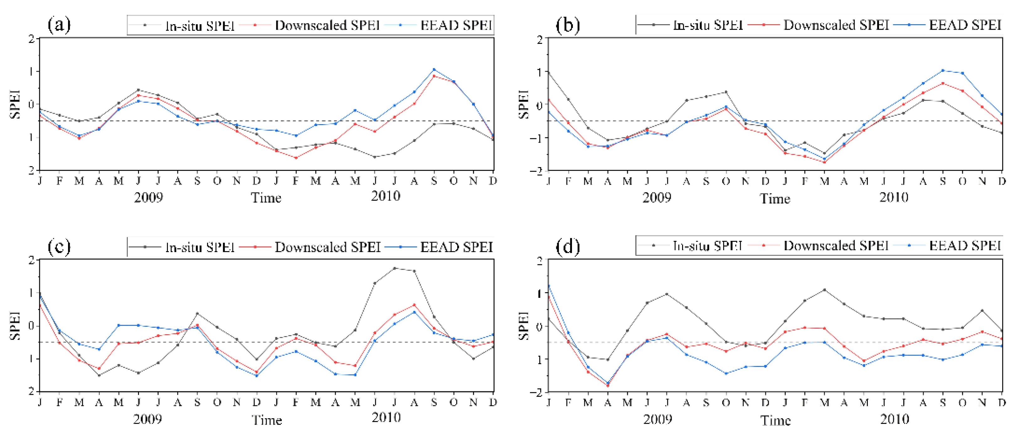
3.3. Direct Validation and Sensitivity Analysis

The direct comparison between the downscaled and in-situ observed SPEI demonstrated a high consistency (R2 = 0.491, MAE = 0.603 and RMSE = 0.773. See Figure 5). This accuracy is very satisfactory considering the scale difference between the downscaled and in-situ observed SPEI.
Southwest China is characterized by a complicated topography. Therefore, we analyzed the topography-dependence of the accuracy. As shown in Figure 6, downscaled SPEI datasets in the region with almost constant elevation are generally more likely to match with in-situ SPEI. However, downscaled SPEI with low R2 can also be identified, mainly distributed in northwest Sichuan, the border of Sichuan eastern plain and Yunnan and the border of Sichuan eastern plain and Guizhou, where there are huge elevation differences. To further illustrate the accuracy variation of the downscaled SPEI with slope, we divided Southwest China into four categories according to slope, i.e., 0–5°, 5–10°, 10–15° and 15–50° and calculated R2 and RMSE in each category (Figure 7). The results show that low slopes result in higher R2 and lower RMSE, especially for 0–5° and 5–10°. In Southwest China, 74.57% of the area is 0–10° and 11.45% of the area is over 15°. These results imply that the downscaled SPEI is reliable and robust in most areas of Southwest China.

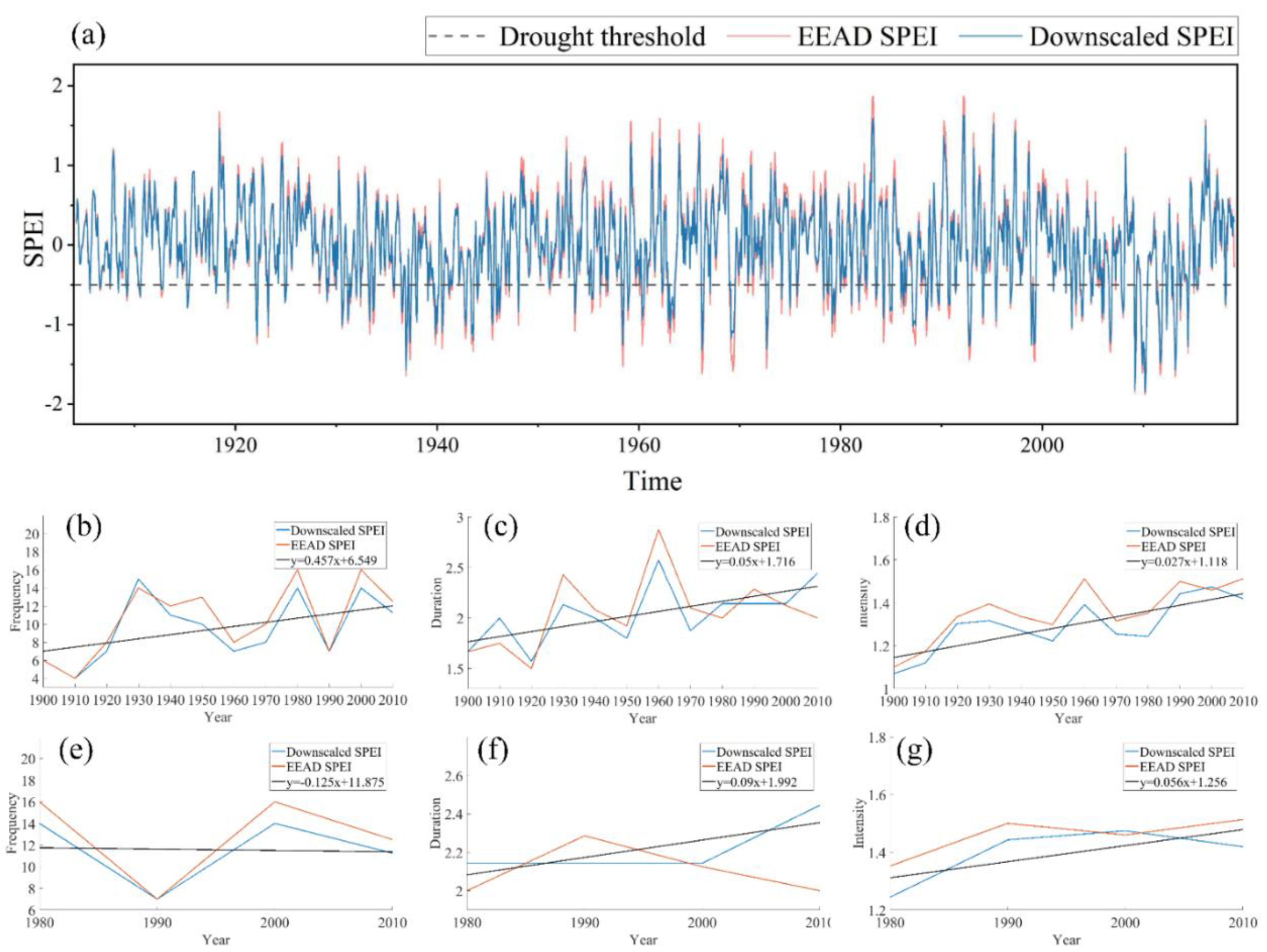
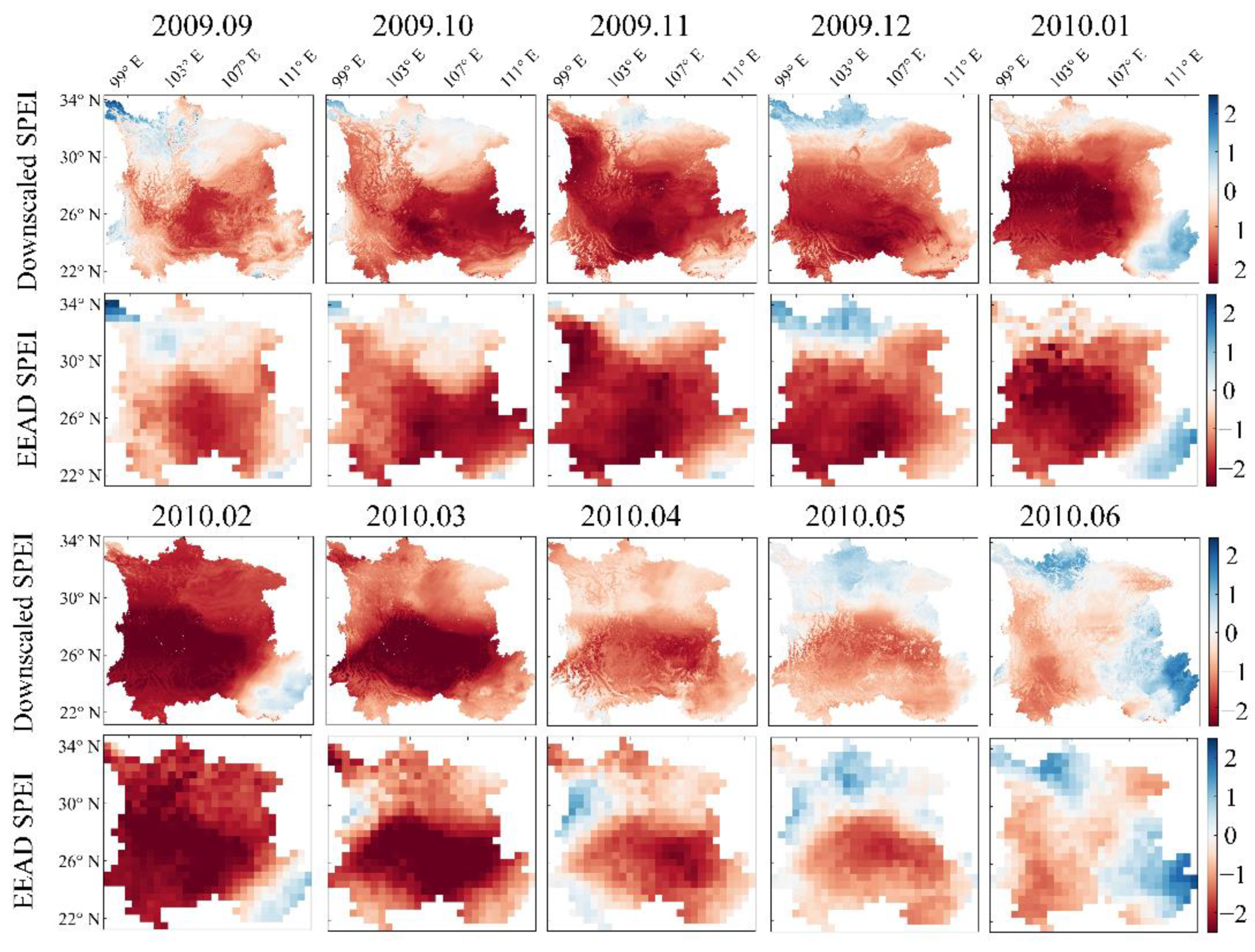
3.4. Derived High-Resolution and Long-Term SPEI Dataset

The temporal behavior of the downscaled SPEI data was compared with the original EEAD SPEI from 1901 to 2018 (Figure 8a). The results show that our downscaled SPEI satisfactorily reproduced the temporal evolution of EEAD over the entire study area. The two products both indicate that Southwest China has presented a rising trend of drought. Figure 8b–d illustrate a slightly increasing trend of drought events in terms of frequency, duration, and intensity. Especially after 1980, there is a dramatically rising trend in terms of duration and frequency, as shown in Figure 8e–g, which is consistent with Wang et al. [23].
There have been many severe drought events in Southwest China, and the 2009/2010 drought event is the most severe one. To evaluate the potential application of the downscaled SPEI data, Figure 9 shows the evolution of this drought episode revealed by downscaled and EEAD SPEI. From a visual perspective, both SPEI maps showed similar spatial distribution patterns over the study area. However, the downscaled high-resolution SPEI data has more spatial details.
To further illustrate the difference between the downscaled SPEI dataset and EEAD, Figure 10 shows their time series and the in-situ SPEI time series during the 2009/2010 drought episode over four selected meteorological stations. Results show that the drought (detected by in-situ measurements) can be well captured by both the downscaled SPEI and the EEAD SPEI data. Close inspection reveals that our downscaled SPEI is closer to the in-situ measurement than the coarse-resolution EEAD product. For example, the in-situ SPEI during November 2009 to September 2010 over site 1 was significantly underestimated by the EEAD, whereas this underestimation was mediated by our downscaled product (Figure 10a). A similar pattern was also found for SPEI from July 2009 to December 2010 over site 4 (Figure 10b).

4. Discussion

More recent work on drought used meteorological station observed data and multiple variables to derive high-resolution datasets based on data-driven models [29,33,53,54]. However, the time span of the in-situ observations and remote sensing data was limited. For example, affected by the time range of MODIS data, the high-resolution integrated surface drought index was obtained, and only the drought events and their impacts from 2001 to 2017 were analyzed [32]. Moreover, the uneven distribution of sites can also greatly affect the relationship model in a small region, and some areas even have no effective sites (e.g., Xinjiang and Guizhou) [60]. In this study, we constructed a relationship model between EEAD SPEI and gridded climate data to downscale the EEAD SPEI. Since VI was not considered as the input, this model supports the generation of SPEI with a longer time span. Based on the model, a 3-month scale SPEI with the longest (1901–2018) time span and the highest spatial resolution over Southwest China was generated. Compared with previous studies, the relationship model without relying on remote sensing data and station data can be applied to any region.
Machine learning has several advantages over traditional statistical methods including the flexibility in handling various data types (e.g., nominal, interval, and ratio); the ability to handle non-parametric data and hierarchical relationships among variables, and the efficient processing of large data volumes [61,62,63]. Tree-based machine learning approaches have been proven to be able to provide more effective local drought information. The evaluation of the SPEI relationship model in our study indicated that an ET-based regression method is better than DT, RF, and GBRT in expressing the complex interaction between SPEI and other surface variables (Figure 3). However, Seonyoung et al. [33] suggested that RF is better than other tree-based algorithms since an ensemble approach was used for preventing an overfitting problem [64]. Verrelst et al. [31] and Upreti et al. [30] give some reasons as to why different research used different machine learning algorithms. When the target variable and the structure of the training dataset are different, the best machine learning algorithm for retrieving biophysical parameters varies. Moreover, huge discrepancies in location and climatic conditions might be another reason. In general, we recommend that different machine learning algorithms are compared when building relational models.
As machine learning methods become ubiquitous, there has been a surge of interest in interpretable machine learning: systems that provide explanations for the relationship between response and driver variables [65]. Gunnar et al. [66], Li et al. [67], and Ben-Ari et al. [68] analyzed the model to reveal the shape of the functional relationship between response and driver variables. In this study, response curves of the models were given (Figure 11) and greatly demonstrated the response of precipitation and temperature to SPEI. Generally, adequate precipitation could ease droughts in most parts, whereas heavy temperature stress tends to worsen droughts event. As seen in Figure 11, the SPEI is monotonously increasing with precipitation at the same temperature. Moreover, temperature mainly affects potential evapotranspiration [69,70]; when the temperature is below 0, there is no potential evapotranspiration [71,72]. In the case of fixed precipitation, temperatures below 0 would not change the SPEI due to low evapotranspiration, whereas the SPEI significantly decreased and drought events were more likely to occur with temperatures beyond 5. In addition, both temperature and precipitation together affected the SPEI. For example, with the increase in precipitation, drought caused by the increasing temperature was alleviated. These observations are consistent with common expectations and textbook knowledge, which means that our model can well describe the relationship between the SPEI and driver variable.
Drought can cause water loss, reducing soil water for a long time which harms vegetation growth [40,73,74]. Consequently, VI, which represents vegetation growth, is a crucial variable for establishing a relationship model with the drought index [32,38,75]. Yang et al. [76] found that there was a significant positive correlation between time-integral NDVI and precipitation in spring and summer over the grasslands. Ji and Peters [77] also found significant correlations between monthly NDVI and SPI during the growing season in the central Great Plains. Similarly, significant correlations between SPEI and NDVI during the growing season were reported by Jiao et al. [78] in water-deficit regions. However, our results indicated that the VI did not significantly improve the accuracy. There are several reasons to explain this phenomenon. Firstly, existing studies have shown that the SPEI is significantly correlated with VI in the growing season, but the growing season only accounted for a small part of our study. Secondly, low correlations between SPEI and NDVI in humid regions were reported by Jiao et al. [78]; most parts of Southwest China are humid or semi-humid areas. Meanwhile, Sumanta et al. [79] found that the R2 for croplands and forests (0.06 and 0.04) were low, and the R2 for grasslands was the highest (0.22) over the United States America. Croplands and forests are the main land cover in Southwest China (Figure 1), whereas grasslands account for only a small part.
The dataset has good performance in monitoring long-term drought events, but there are still some limitations that may affect the performance of the dataset. On the one hand, there is no absolute “real” drought measure [80]. Although this downscaled SPEI dataset is more consistent with in-situ data, it does not provide a true validation of drought events. On the other hand, it is difficult to obtain accurate temperature and precipitation data over mountainous areas. Therefore, in our study, there is a low correlation between the predicted SPEI and in-situ SPEI over a slope greater than 15° (Figure 7). In future work, we would focus on improving the accuracy of the SPEI in complex terrain areas with steep slopes.

5. Conclusions

In this study, four machine learning approaches (DT, RF, GBRT, and ET) were compared in constructing the relationship between climate data and the SPEI. Meanwhile, the importance of VI as an input variable in SPEI reconstruction was assessed. The climate data and auxiliary data were applied to establish the downscaled SPEI dataset in Southwest China from 1901 to 2018 using an ET algorithm. The spatial-temporal characteristics of the 2009–2010 drought were compared with 0.5° EEAD SPEI. The results can be summarized as follows: (1) Among the four machine learning methods, the ET-based algorithm showed the best performance (R2 = 0.889, MAE = 0.232, and RMSE = 0.432); and (2) VI had no significant effect on SPEI reconstruction. Based on climate data and auxiliary data, a high-resolution (1 km) and long-term (1901 to 2018) SPEI dataset over Southwest China using an ET algorithm was generated. The downscaled SPEI dataset is more consistent with in-situ SPEI compared to the 0.5° EEAD SPEI. In addition, the downscaled SPEI dataset was slope-dependent: the accuracy increases as the slope decreases.
Overall, we provided a new and reliable way to overcome the temporal limitation of input data and generate high-resolution and long-term drought products even with limited VI data availability. As an important response variable to drought, VI needs to be carefully applied to reconstruct the drought index. Our product is expected to provide a reference for long-term regional drought monitoring.

Author Contributions

Conceptualization, G.Y.; methodology, R.F.; validation, R.F., X.C. and H.G.; resources, C.W. (Cong Wang) and G.L.; writing—original draft preparation, R.F.; writing—review and editing, G.Y., B.X., R.C., C.W. (Changjing Wang) and X.C. All authors have read and agreed to the published version of the manuscript.

Funding

This research was funded by the Sichuan Science and Technology Program (2021JDJQ0007, 2020JDTD0003), the National Natural Science Foundation of China (41971282, 42101391), Natural Science Foundation of Fujian Province (Grant No. 2019J01853), and the Fundamental Research Funds for the Central Universities (2662021JC013, CCNU21XJ028).

Institutional Review Board Statement

Not applicable.

Informed Consent Statement

Not applicable.

Data Availability Statement

The data presented in this study are available on request from the authors.

Conflicts of Interest

The authors declare no conflict of interest. The funders had no role in the design of the study; in the collection, analyses, or interpretation of data; in the writing of the manuscript, or in the decision to publish the results.

References

  1. Wilhite, D.A. Preparing for Drought: A Methodology; University of Nebraska Lincoln: Lincoln, NE, USA, 2000. [Google Scholar]
  2. Li, J.; Wang, Z.; Wu, X.; Zscheischler, J.; Guo, S.; Chen, X.J.H.; Sciences, E.S. A standardized index for assessing sub-monthly compound dry and hot conditions with application in China. Hydrol. Earth Syst. Sci. 2021, 25, 1587–1601. [Google Scholar] [CrossRef]
  3. Williams, A.P.; Cook, E.R.; Smerdon, J.E.; Cook, B.I.; Abatzoglou, J.T.; Bolles, K.; Baek, S.H.; Badger, A.M.; Livneh, B.J.S. Large contribution from anthropogenic warming to an emerging North American megadrought. Science 2020, 368, 314–318. [Google Scholar] [CrossRef]
  4. Duan, R.; Huang, G.; Li, Y.; Zhou, X.; Ren, J.; Tian, C.J.E.R. Stepwise clustering future meteorological drought projection and multi-level factorial analysis under climate change: A case study of the Pearl River Basin, China. Environ. Res. 2021, 196, 110368. [Google Scholar] [CrossRef] [PubMed]
  5. Tabari, H.; Hosseinzadehtalaei, P.; Thiery, W.; Willems, P.J.E.S.F. Amplified drought and flood risk under future socioeconomic and climatic change. Earths Future 2021, 9, e2021EF002295. [Google Scholar] [CrossRef]
  6. Balti, H.; Abbes, A.B.; Mellouli, N.; Farah, I.R.; Sang, Y.; Lamolle, M. A review of drought monitoring with big data: Issues, methods, challenges and research directions. Ecol. Inform. 2020, 60, 101136. [Google Scholar] [CrossRef]
  7. Gavahi, K.; Abbaszadeh, P.; Moradkhani, H.; Zhan, X.; Hain, C. Multivariate assimilation of remotely sensed soil moisture and evapotranspiration for drought monitoring. J. Hydrometeorol. 2020, 21, 2293–2308. [Google Scholar] [CrossRef]
  8. Gao, Z.; Wang, Q.; Cao, X.; Gao, W. The responses of vegetation water content (EWT) and assessment of drought monitoring along a coastal region using remote sensing. GISci. Remote Sens. 2014, 51, 1–16. [Google Scholar] [CrossRef]
  9. Manalo, J.A., IV; van de Fliert, E.; Fielding, K. Rice farmers adapting to drought in the Philippines. Int. J. Agric. Sustain. 2020, 18, 594–605. [Google Scholar] [CrossRef]
  10. Kim, T.-W.; Jehanzaib, M. Drought risk analysis, forecasting and assessment under climate change. Water 2020, 12, 1862. [Google Scholar] [CrossRef]
  11. Orimoloye, I.R.; Belle, J.A.; Olusola, A.O.; Busayo, E.T.; Ololade, O.O. Spatial assessment of drought disasters, vulnerability, severity and water shortages: A potential drought disaster mitigation strategy. Nat. Hazards 2021, 105, 2735–2754. [Google Scholar] [CrossRef]
  12. McKee, T.B.; Doesken, N.J.; Kleist, J. The relationship of drought frequency and duration to time scales. In Proceedings of the 8th Conference on Applied Climatology, Anaheim, CA, USA, 17–22 January 1993; pp. 179–183. [Google Scholar]
  13. Shukla, S.; Wood, A.W. Use of a standardized runoff index for characterizing hydrologic drought. Geophys. Res. Lett. 2008, 35, L02405. [Google Scholar] [CrossRef] [Green Version]
  14. AghaKouchak, A.J.H.; Sciences, E.S. A baseline probabilistic drought forecasting framework using standardized soil moisture index: Application to the 2012 United States drought. Hydrol. Earth Syst. Sci. 2014, 18, 2485–2492. [Google Scholar] [CrossRef] [Green Version]
  15. Xu, L.; Chen, N.; Yang, C.; Zhang, C.; Yu, H.J.A.; Meteorology, F. A parametric multivariate drought index for drought monitoring and assessment under climate change. Agric. For. Meteorol. 2021, 310, 108657. [Google Scholar] [CrossRef]
  16. Dixit, S.; Jayakumar, K.V. Spatio-temporal analysis of copula-based probabilistic multivariate drought index using CMIP6 model. Int. J. Clim. 2021. [Google Scholar] [CrossRef]
  17. Yisehak, B.; Zenebe, A. Modeling multivariate standardized drought index based on the drought information from precipitation and runoff: A case study of Hare watershed of Southern Ethiopian Rift Valley Basin. Model. Earth Syst. Environ. 2021, 7, 1005–1017. [Google Scholar] [CrossRef]
  18. Palmer, W.C. Meteorological Drought; US Department of Commerce, Weather Bureau: Washington, DC, USA, 1965; Volume 30. [Google Scholar]
  19. Vicente-Serrano, S.M.; Beguería, S.; López-Moreno, J.I. A multiscalar drought index sensitive to global warming: The standardized precipitation evapotranspiration index. J. Clim. 2010, 23, 1696–1718. [Google Scholar] [CrossRef] [Green Version]
  20. Pei, Z.; Fang, S.; Wang, L.; Yang, W. Comparative analysis of drought indicated by the SPI and SPEI at various timescales in inner Mongolia, China. Water 2020, 12, 1925. [Google Scholar] [CrossRef]
  21. Hao, C.; Zhang, J.; Yao, F. Combination of multi-sensor remote sensing data for drought monitoring over Southwest China. Int. J. Appl. Earth Obs. Geoinf. 2015, 35, 270–283. [Google Scholar] [CrossRef]
  22. Li, X.; Li, Y.; Chen, A.; Gao, M.; Slette, I.J.; Piao, S.J.A.; Meteorology, F. The impact of the 2009/2010 drought on vegetation growth and terrestrial carbon balance in Southwest China. Agric. For. Meteorol. 2019, 269, 239–248. [Google Scholar] [CrossRef]
  23. Wang, M.; Ding, Z.; Wu, C.; Song, L.; Ma, M.; Yu, P.; Lu, B.; Tang, X. Divergent responses of ecosystem water-use efficiency to extreme seasonal droughts in Southwest China. Sci. Total Environ. 2021, 760, 143427. [Google Scholar] [CrossRef]
  24. Zeng, Z.; Wu, W.; Ge, Q.; Li, Z.; Wang, X.; Zhou, Y.; Zhang, Z.; Li, Y.; Huang, H.; Liu, G.J.A.; et al. Legacy effects of spring phenology on vegetation growth under preseason meteorological drought in the Northern Hemisphere. Agric. For. Meteorol. 2021, 310, 108630. [Google Scholar] [CrossRef]
  25. Lloyd-Hughes, B. A spatio-temporal structure-based approach to drought characterisation. Int. J. Clim. 2012, 32, 406–418. [Google Scholar] [CrossRef] [Green Version]
  26. Xu, K.; Yang, D.; Yang, H.; Li, Z.; Qin, Y.; Shen, Y. Spatio-temporal variation of drought in China during 1961–2012: A climatic perspective. J. Hydrol. 2015, 526, 253–264. [Google Scholar] [CrossRef]
  27. Lotfirad, M.; Esmaeili-Gisavandani, H.; Adib, A. Drought monitoring and prediction using SPI, SPEI, and random forest model in various climates of Iran. Water Clim. Chang. 2022, 13, 383–406. [Google Scholar] [CrossRef]
  28. Han, H.; Bai, J.; Yan, J.; Yang, H.; Ma, G. A combined drought monitoring index based on multi-sensor remote sensing data and machine learning. Geocarto Int. 2021, 36, 1161–1177. [Google Scholar] [CrossRef]
  29. Greifeneder, F.; Notarnicola, C.; Wagner, W. A machine learning-based approach for surface soil moisture estimations with google earth engine. Remote Sens. 2021, 13, 2099. [Google Scholar] [CrossRef]
  30. Upreti, D.; Huang, W.; Kong, W.; Pascucci, S.; Pignatti, S.; Zhou, X.; Ye, H.; Casa, R. A comparison of hybrid machine learning algorithms for the retrieval of wheat biophysical variables from sentinel-2. Remote Sens. 2019, 11, 481. [Google Scholar] [CrossRef] [Green Version]
  31. Verrelst, J.; Muñoz, J.; Alonso, L.; Delegido, J.; Rivera, J.P.; Camps-Valls, G.; Moreno, J. Machine learning regression algorithms for biophysical parameter retrieval: Opportunities for Sentinel-2 and-3. Remote Sens. Environ. 2012, 118, 127–139. [Google Scholar] [CrossRef]
  32. Jiang, W.; Wang, L.; Zhang, M.; Yao, R.; Chen, X.; Gui, X.; Sun, J.; Cao, Q. Analysis of drought events and their impacts on vegetation productivity based on the integrated surface drought index in the Hanjiang River Basin, China. Atmos. Res. 2021, 254, 105536. [Google Scholar] [CrossRef]
  33. Park, S.; Im, J.; Jang, E.; Rhee, J. Drought assessment and monitoring through blending of multi-sensor indices using machine learning approaches for different climate regions. Agric. For. Meteorol. 2016, 216, 157–169. [Google Scholar] [CrossRef]
  34. Rahmati, O.; Falah, F.; Dayal, K.S.; Deo, R.C.; Mohammadi, F.; Biggs, T.; Moghaddam, D.D.; Naghibi, S.A.; Bui, D.T. Machine learning approaches for spatial modeling of agricultural droughts in the south-east region of Queensland Australia. Sci. Total Environ. 2020, 699, 134230. [Google Scholar] [CrossRef] [PubMed]
  35. Son, B.; Park, S.; Im, J.; Park, S.; Ke, Y.; Quackenbush, L.J. A new drought monitoring approach: Vector Projection Analysis (VPA). Remote Sens. Environ. 2021, 252, 112145. [Google Scholar] [CrossRef]
  36. Zhao, W.; Sánchez, N.; Lu, H.; Li, A. A spatial downscaling approach for the SMAP passive surface soil moisture product using random forest regression. J. Hydrol. 2018, 563, 1009–1024. [Google Scholar] [CrossRef]
  37. Im, J.; Park, S.; Rhee, J.; Baik, J.; Choi, M. Downscaling of AMSR-E soil moisture with MODIS products using machine learning approaches. Environ. Earth Sci. 2016, 75, 1120. [Google Scholar] [CrossRef]
  38. Brown, J.F.; Wardlow, B.D.; Tadesse, T.; Hayes, M.J.; Reed, B.C. The Vegetation Drought Response Index (VegDRI): A new integrated approach for monitoring drought stress in vegetation. GISci. Remote Sens. 2008, 45, 16–46. [Google Scholar] [CrossRef]
  39. Wu, J.; Zhou, L.; Liu, M.; Zhang, J.; Leng, S.; Diao, C. Establishing and assessing the Integrated Surface Drought Index (ISDI) for agricultural drought monitoring in mid-eastern China. Int. J. Appl. Earth Obs. Geoinf. 2013, 23, 397–410. [Google Scholar] [CrossRef]
  40. Liu, D.; Zhang, C.; Ogaya, R.; Estiarte, M.; Peñuelas, J. Effects of decadal experimental drought and climate extremes on vegetation growth in Mediterranean forests and shrublands. J. Veg. Sci. 2020, 31, 768–779. [Google Scholar] [CrossRef]
  41. Zhu, X.; Xiao, G.; Zhang, D.; Guo, L. Mapping abandoned farmland in China using time series MODIS NDVI. Sci. Total Environ. 2021, 755, 142651. [Google Scholar] [CrossRef] [PubMed]
  42. Pei, F.; Zhou, Y.; Xia, Y. Application of normalized difference vegetation index (NDVI) for the detection of extreme precipitation change. Forests 2021, 12, 594. [Google Scholar] [CrossRef]
  43. Sanz, E.; Saa-Requejo, A.; Díaz-Ambrona, C.H.; Ruiz-Ramos, M.; Rodríguez, A.; Iglesias, E.; Esteve, P.; Soriano, B.; Tarquis, A. Normalized Difference Vegetation Index Temporal Responses to Temperature and Precipitation in Arid Rangelands. Remote Sens. 2021, 13, 840. [Google Scholar] [CrossRef]
  44. Mokhtar, A.; He, H.; Alsafadi, K.; Mohammed, S.; He, W.; Li, Y.; Zhao, H.; Abdullahi, N.M.; Gyasi-Agyei, Y. Ecosystem water use efficiency response to drought over southwest China. Ecohydrology 2021, e2317. [Google Scholar] [CrossRef]
  45. Cheng, Q.; Gao, L.; Zhong, F.; Zuo, X.; Ma, M. Spatiotemporal variations of drought in the Yunnan-Guizhou Plateau, southwest China, during 1960–2013 and their association with large-scale circulations and historical records. Ecol. Indic. 2020, 112, 106041. [Google Scholar] [CrossRef]
  46. Piao, S.; Fang, J.; Ciais, P.; Peylin, P.; Huang, Y.; Sitch, S.; Wang, T. The carbon balance of terrestrial ecosystems in China. Nature 2009, 458, 1009–1013. [Google Scholar] [CrossRef]
  47. Zhuo, Z.; Chen, Q.; Zhang, X.; Chen, S.; Gou, Y.; Sun, Z.; Huang, Y.; Shi, Z. Soil organic carbon storage, distribution, and influencing factors at different depths in the dryland farming regions of Northeast and North China. CATENA 2022, 210, 105934. [Google Scholar] [CrossRef]
  48. Qiu, J. China drought highlights future climate threats. Natuer 2010, 465, 142–143. [Google Scholar] [CrossRef] [Green Version]
  49. Lai, P.; Zhang, M.; Ge, Z.; Hao, B.; Song, Z.; Huang, J.; Ma, M.; Yang, H.; Han, X. Responses of seasonal indicators to extreme droughts in Southwest China. Remote Sens. 2020, 12, 818. [Google Scholar] [CrossRef] [Green Version]
  50. Allen, R.; Pereira, L.; Raes, D.; Smith, M.; Allen, R.G.; Pereira, L.S.; Martin, S.J.F. Crop Evapotranspiration: Guidelines for Computing Crop Water Requirements; FAO Irrigation and Drainage Paper 56; FAO: Rome, Italy, 1998; Volume 56. [Google Scholar]
  51. Peng, S.; Ding, Y.; Liu, W.; Li, Z. 1 km monthly temperature and precipitation dataset for China from 1901 to 2017. Earth Syst. Sci. Data 2019, 11, 1931–1946. [Google Scholar] [CrossRef] [Green Version]
  52. Galvao, L.S.; dos Santos, J.R.; Roberts, D.A.; Breunig, F.M.; Toomey, M.; de Moura, Y.M. On intra-annual EVI variability in the dry season of tropical forest: A case study with MODIS and hyperspectral data. Remote Sens. Environ. 2011, 115, 2350–2359. [Google Scholar] [CrossRef]
  53. Shamshirband, S.; Hashemi, S.; Salimi, H.; Samadianfard, S.; Asadi, E.; Shadkani, S.; Kargar, K.; Mosavi, A.; Nabipour, N.; Chau, K.-W. Predicting standardized streamflow index for hydrological drought using machine learning models. Eng. Appl. Comput. Fluid Mech. 2020, 14, 339–350. [Google Scholar] [CrossRef]
  54. Aghelpour, P.; Bahrami-Pichaghchi, H.; Varshavian, V. Hydrological drought forecasting using multi-scalar streamflow drought index, stochastic models and machine learning approaches, in northern Iran. Stoch. Hydrol. Hydraul. 2021, 35, 1615–1635. [Google Scholar] [CrossRef]
  55. Kabilan, R.; Chandran, V.; Yogapriya, J.; Karthick, A.; Gandhi, P.P.; Mohanavel, V.; Rahim, R.; Manoharan, S. Short-term power prediction of building integrated photovoltaic (BIPV) system based on machine learning algorithms. Int. J. Photoenergy 2021, 2021, 5582418. [Google Scholar] [CrossRef]
  56. Chicco, D.; Warrens, M.J.; Jurman, G. The coefficient of determination R-squared is more informative than SMAPE, MAE, MAPE, MSE and RMSE in regression analysis evaluation. PeerJ Comput. Sci. 2021, 7, e623. [Google Scholar] [CrossRef]
  57. Ukkola, A.M.; De Kauwe, M.G.; Roderick, M.L.; Abramowitz, G.; Pitman, A.J. Robust future changes in meteorological drought in CMIP6 projections despite uncertainty in precipitation. Geophys. Res. Lett. 2020, 47, e2020GL087820. [Google Scholar] [CrossRef]
  58. Ali, J.; Khan, R.; Ahmad, N.; Maqsood, I. Random forests and decision trees. Int. J. Comput. Sci. Issues 2012, 9, 272. [Google Scholar]
  59. Elith, J.; Leathwick, J.R.; Hastie, T. A working guide to boosted regression trees. J. Anim. Ecol. 2008, 77, 802–813. [Google Scholar] [CrossRef] [PubMed]
  60. Wang, Q.; Zeng, J.; Qi, J.; Zhang, X.; Zeng, Y.; Shui, W.; Xu, Z.; Zhang, R.; Wu, X. A Multi-Scale Daily SPEI Dataset for Drought Monitoring at Observation Stations over the Mainland China from 1961 to 2018. Earth Syst. Sci. Data 2020, 13, 331–341. [Google Scholar] [CrossRef]
  61. De’ath, G.; Fabricius, K.E. Classification and regression trees: A powerful yet simple technique for ecological data analysis. Ecol. Ecol. Soc. Am. 2000, 81, 3178–3192. [Google Scholar] [CrossRef]
  62. Ao, Y.; Li, H.; Zhu, L.; Ali, S.; Yang, Z. The linear random forest algorithm and its advantages in machine learning assisted logging regression modeling. J. Pet. Sci. Eng. 2019, 174, 776–789. [Google Scholar] [CrossRef]
  63. Khanzode, K.C.A.; Sarode, R.D. Advantages and Disadvantages of Artificial Intelligence and Machine Learning: A Literature Review. Int. J. Libr. Inf. Sci. 2020, 9, 3. [Google Scholar]
  64. Prasad, A.M.; Iverson, L.R.; Liaw, A. Newer classification and regression tree techniques: Bagging and random forests for ecological prediction. Ecosystems 2006, 9, 181–199. [Google Scholar] [CrossRef]
  65. Doshi-Velez, F.; Kim, B. Towards a rigorous science of interpretable machine learning. arXiv 2017, arXiv:1702.08608. [Google Scholar]
  66. Lischeid, G.; Webber, H.; Sommer, M.; Nendel, C.; Ewert, F. Machine learning in crop yield modelling: A powerful tool, but no surrogate for science. Agric. For. Meteorol. 2022, 312, 108698. [Google Scholar] [CrossRef]
  67. Li, Y.; Guan, K.; Schnitkey, G.D.; DeLucia, E.; Peng, B. Excessive rainfall leads to maize yield loss of a comparable magnitude to extreme drought in the United States. Glob. Chang. Biol. 2019, 25, 2325–2337. [Google Scholar] [CrossRef] [Green Version]
  68. Ben-Ari, T.; Adrian, J.; Klein, T.; Calanca, P.; Van der Velde, M.; Makowski, D. Identifying indicators for extreme wheat and maize yield losses. Agric. For. Meteorol. 2016, 220, 130–140. [Google Scholar] [CrossRef]
  69. Xiang, K.; Li, Y.; Horton, R.; Feng, H. Similarity and difference of potential evapotranspiration and reference crop evapotranspiration—A review. Agric. Water Manag. 2020, 232, 106043. [Google Scholar] [CrossRef]
  70. Basso, B.; Martinez-Feria, R.A.; Rill, L.; Ritchie, J.T. Contrasting long-term temperature trends reveal minor changes in projected potential evapotranspiration in the US Midwest. Nat. Commun. 2021, 12, 1476. [Google Scholar] [CrossRef] [PubMed]
  71. Adnan, R.M.; Heddam, S.; Yaseen, Z.M.; Shahid, S.; Kisi, O.; Li, B. Prediction of potential evapotranspiration using temperature-based heuristic approaches. Sustainability 2020, 13, 297. [Google Scholar] [CrossRef]
  72. Han, J.; Wang, J.; Zhao, Y.; Wang, Q.; Zhang, B.; Li, H.; Zhai, J. Spatio-temporal variation of potential evapotranspiration and climatic drivers in the Jing-Jin-Ji region, North China. Agric. For. Meteorol. 2018, 256, 75–83. [Google Scholar] [CrossRef]
  73. Rhee, J.; Im, J.; Park, S. Regional drought monitoring based on multi-sensor remote sensing. In Remote Sensing of Water Resources, Disasters, and Urban Studies; Thenkabail, P.S., Ed.; CRC Press: Boca Raton, FL, USA, 2014; pp. 401–415. [Google Scholar]
  74. Jiang, P.; Ding, W.; Yuan, Y.; Ye, W. Diverse response of vegetation growth to multi-time-scale drought under different soil textures in China’s pastoral areas. J. Environ. Manag. 2020, 274, 110992. [Google Scholar] [CrossRef]
  75. Wu, J.; Zhou, L.; Mo, X.; Zhou, H.; Zhang, J.; Jia, R. Drought monitoring and analysis in China based on the Integrated Surface Drought Index (ISDI). Int. J. Appl. Earth Obs. Geoinf. 2015, 41, 23–33. [Google Scholar] [CrossRef]
  76. Yang, L.; Wylie, B.K.; Tieszen, L.L.; Reed, B.C. An analysis of relationships among climate forcing and time-integrated NDVI of grasslands over the US northern and central Great Plains. Remote Sens. Environ. 1998, 65, 25–37. [Google Scholar] [CrossRef]
  77. Ji, L.; Peters, A.J. Assessing vegetation response to drought in the northern Great Plains using vegetation and drought indices. Remote Sens. Environ. 2003, 87, 85–98. [Google Scholar] [CrossRef]
  78. Jiao, W.; Wang, L.; Smith, W.K.; Chang, Q.; Wang, H.; D’Odorico, P. Observed increasing water constraint on vegetation growth over the last three decades. Nat. Commun. 2021, 12, 3777. [Google Scholar] [CrossRef]
  79. Chatterjee, S.; Desai, A.R.; Zhu, J.; Townsend, P.A.; Huang, J. Soil moisture as an essential component for delineating and forecasting agricultural rather than meteorological drought. Remote Sens. Environ. 2022, 269, 112833. [Google Scholar] [CrossRef]
  80. Jiao, W.; Tian, C.; Chang, Q.; Novick, K.A.; Wang, L. A new multi-sensor integrated index for drought monitoring. Agric. For. Meteorol. 2019, 268, 74–85. [Google Scholar] [CrossRef] [Green Version]
Figure 1. Land cover in our study area. The meteorological stations used for validation were also shown.
Remotesensing 14 01662 g001
Figure 2. Flowchart of the downscaling procedure in this study.
Remotesensing 14 01662 g002
Figure 3. Density scatter plot between EEAD and predicted SPEI based on (a) DT, (b) RF, (c) GBRT, and (d) ET. Results are from cross-validation.
Remotesensing 14 01662 g003
Figure 4. Density scatter plot between EEAD and estimated SPEI from Extra Trees (ET) with (a) both gridded climate data and vegetation index (VI) as input, and (b) with only gridded climate data as input. Results are from cross-validation.
Remotesensing 14 01662 g004
Figure 5. Density scatter plot between estimated and in-situ SPEI.
Remotesensing 14 01662 g005
Figure 6. Spatial distribution of coefficient of determination (R2) between the downscaled SPEI and in-situ SPEI at each meteorological station.
Remotesensing 14 01662 g006
Figure 7. Boxplot summarizing the sensitivity of predicted SPEI to slope: (a) R2 and (b) RMSE.
Remotesensing 14 01662 g007
Figure 8. The temporal evolution of SPEI and interdecadal changes of the frequency, duration and intensity of drought events from 1901 to 2018 and 1980 to 2018: (a) the time series of SPEI; (b) the frequency of drought events from 1901 to 2018; (c) the duration of drought events from 1901 to 2018; (d) the intensity of drought events from 1980 to 2018; (e) the frequency of drought events; (f) the duration of drought events from 1980 to 2018; (g) the intensity of drought events from 1980 to 2018. Black line in b-g is the trend of downscaled SPEI.
Remotesensing 14 01662 g008
Figure 9. Drought conditions in Southwest China monitored by downscaled SPEI and EEAD SPEI from September 2009 to June 2011. The first and third rows display the downscaled SPEI, and the second and fourth rows show the EEAD SPEI.
Remotesensing 14 01662 g009
Figure 10. Time series of the in-situ SPEI, downscaled SPEI, and EEAD at the four selected meteorological stations. Panels (ad) are site 1–4, respectively.
Remotesensing 14 01662 g010
Figure 11. Dependence of the downscaled SPEI on precipitation and temperature.
Remotesensing 14 01662 g011
Table 1. Information about the data used in this study.
TypeNameResolutionSource
In-situ climatePrecipitationstationhttp://data.tpdc.ac.cn/zh-hans/ (accessed on 12 February 2022)
Temperaturestationhttp://data.tpdc.ac.cn/zh-hans/ (accessed on 12 February 2022)
Windstationhttp://data.tpdc.ac.cn/zh-hans/ (accessed on 12 February 2022)
Sunshine durationstationhttp://data.tpdc.ac.cn/zh-hans/ (accessed on 12 February 2022)
Gridded climatePrecipitation1 kmhttp://data.tpdc.ac.cn/zh-hans/ (accessed on 12 February 2022)
Temperature1 kmhttp://data.tpdc.ac.cn/zh-hans/ (accessed on 12 February 2022)
Standardized Precipitation Evapotranspiration Index0.5°https://digital.csic.es/handle/10261/202305 (accessed on 12 February 2022)
MODIS dataEnhanced Vegetation Index500 mhttps://ladsweb.modaps.eosdis.nasa.gov/ (accessed on 12 February 2022)
Normalized Difference Vegetation Index500 mhttps://ladsweb.modaps.eosdis.nasa.gov/ (accessed on 12 February 2022)
Topographic dataDigital elevation model1 kmhttp://www.resdc.cn/ (accessed on 12 February 2022)
Publisher’s Note: MDPI stays neutral with regard to jurisdictional claims in published maps and institutional affiliations.

