New Evidence Supporting the Pacific Mantle Outflow: Hints from Crustal Magnetization of the Phoenix Plate

Abstract

Magnetic contributions to the Earth’s magnetic field within the lithosphere are known as magnetic anomalies. Magnetic anomaly maps provide insight on magnetic properties of subsurface rock, geological structures, and plate tectonic history. A small number of studies have analyzed the Phoenix Plate based on magnetic anomaly data. These focused on its tectonic evolution. Here, we study the crustal magnetization of this region and combine the results with additional information from high-resolution bathymetry and complete Bouguer gravity anomalies. We analyzed the horizontal variation of the magnetization in two spectral domains: one that resolves the medium and long wavelengths magnetization components (20–200 km), and another one that focuses on short wavelengths (7–100 km). The obtained magnetization amplitude for the 20–200 km range reveals the presence of NE–SW and NW–SE high trends in magnetization. We attribute these alignments to induced magnetism. For the range of 7–100 km, the magnetization amplitude shows a progressive decrease towards the southern part of the Phoenix Plate. The obtained magnetization pattern and the integration with additional geophysical and geological information indicates a thermal demagnetization of the oceanic crust in the south, possibly caused by the Pacific mantle outflow present in this region.

1. Introduction

Magnetic measurements at or near Earth’s surface detect fields from several sources. More than 90% of the signal comes from the Earth’s main magnetic field. The other 10% is related to external fields and magnetic minerals. The latest generate magnetic anomalies in the lithosphere. Magnetic anomaly maps provide information regarding the thermal structure of the lithosphere, plate tectonic history, and the location and distribution of natural resources. Particularly, the study of magnetic data on a regional compilation can be used to reveal the main tectonic elements and the associated geological processes and history.

The opening of the Drake Passage involved the final breakup of the Gondwana supercontinent and gave way to the development of the Scotia Arc. The Scotia Sea, located between South America and Antarctica, is presently constituted by the Scotia and Sandwich plates. The Scotia Arc is surrounded by the former Phoenix Plate to the west, the Antarctic Plate to the south, and the South American Plate in the remaining sites (Figure 1). The structure that accommodates the movements between the Scotia Plate and the Phoenix Plate is an oceanic transverse ridge known as the Shackleton Fracture Zone (SFZ) [1].

The Pacific side of the Antarctic Peninsula shows, through the pattern of its magnetic anomalies, an east-directed subduction history dominated by the arrival of successive ridge segments at the subduction trench. The end of the spreading at the Phoenix Plate and the capture of subducting microplates along the east Antarctic Pacific margin was developed from the Early Cenozoic (50 Ma) until 4 Ma and it was a progressive process from the south to the north [2,3].

The Phoenix Plate was formed by seafloor spreading since the Jurassic, as one of the major Pacific Ocean plates. It is bounded at the NE and SW by two major oceanic fracture zones: the Shackleton and the Hero Fracture Zones, respectively (Figure 1b: dotted black lines labeled as SFZ and HFZ). The southern part of the Phoenix Plate bounds with the South Shetlands Trench and the South Shetland archipelago block. Apart from the SFZ and HFZ, three other discontinuities segmented the mid-ocean ridge structure into three tectonic blocks, known as oceanic corridors. These three oceanic corridors became inactive after the collisions between more southerly ridge segments and a subduction zone south of the Hero Fracture Zone [4,5].

Figure 1. Scotia Sea and study area. (a) General bathymetry map of the Scotia Sea. Plate boundaries in thick white curvilinear lines. AP: Antarctic Peninsula. DP: Drake’s Passage. PP: Phoenix Plate. SP: Sandwich Plate. WS: Weddell Sea. PB: Powell Basin. (b) P1, P2, and P3 denote the three inactive plate segments of the Phoenix Ridge. SSA: South Shetland archipelago. SST: South Shetland Trench. SI: Smith Island. A black solid irregular polygon highlights the flexural bulge. Two white thin lines separate P1, P2, and P3 zones. In upper or lower figures: A white rectangle highlights the study area. HFZ: Hero Fracture Zone. SFZ: Shackleton Fracture Zone. Both fracture zones are depicted with solid white lines (upper panel) and thin black lines (lower panel). Two sources of topographic/bathymetry data were used here: the SRTM30 Plus v7 [6] for the background image, and the new digital bathymetric model with 200 m spatial resolution [7] for the study area. The later one is delimited by a black solid circular sector. 1: Transcurrent faults.

Figure 1. Scotia Sea and study area. (a) General bathymetry map of the Scotia Sea. Plate boundaries in thick white curvilinear lines. AP: Antarctic Peninsula. DP: Drake’s Passage. PP: Phoenix Plate. SP: Sandwich Plate. WS: Weddell Sea. PB: Powell Basin. (b) P1, P2, and P3 denote the three inactive plate segments of the Phoenix Ridge. SSA: South Shetland archipelago. SST: South Shetland Trench. SI: Smith Island. A black solid irregular polygon highlights the flexural bulge. Two white thin lines separate P1, P2, and P3 zones. In upper or lower figures: A white rectangle highlights the study area. HFZ: Hero Fracture Zone. SFZ: Shackleton Fracture Zone. Both fracture zones are depicted with solid white lines (upper panel) and thin black lines (lower panel). Two sources of topographic/bathymetry data were used here: the SRTM30 Plus v7 [6] for the background image, and the new digital bathymetric model with 200 m spatial resolution [7] for the study area. The later one is delimited by a black solid circular sector. 1: Transcurrent faults.

Maldonado et al. [8], on the basis of surface marine magnetics, multichannel seismic, long-range side-scan sonar, and multibeam bathymetry, studied the contact between the Phoenix Plate and South Shetland Islands block. They described the main features: the trench, the accretionary prism, and the outer flexural bulge related to the subduction process. In their study, they reconstructed the convergence history of the trench. They marked a constant convergence rate of 40 to 60 mm/y up to 6.7 Ma. Later, it rapidly decreased to less than 10 mm/y. They also proposed that the current elevation of Smith Island is a consequence of the ridge crest-trench collision that took place directly southwest of the HFZ 5.5 Ma.

Based on bathymetric and magnetic anomaly data, Livermore et al. [5] supported that the extinction of the three remaining segments occurred 3.3 ± 0.2 Ma. In addition, Eagles [9] performed a study based on a joint inversion of magnetic isochron and fracture zone data in these three extinct spreading segments. He detected falling spreading rates between magnetic anomaly chrons C4 (~8.1 Ma) and C2A (~3.3 Ma) when the ridge became inactive. Jin et al. [10], using swath bathymetry, gravity, and magnetic data, performed a study focused on one of the three remaining segments, the so-called P3. They proposed that the cessation of P3 spreading occurred at about 3.6 Ma.

The aim of this paper is to provide a new magnetic perspective of the Phoenix Plate. For this, it is key to understand that the magnetic structure of the oceanic crust follows a regular architecture in its mineral composition. Note that rocks magnetization depends on composition of magnetic minerals, and temperature. Since most of the minerals are paramagnetic or diamagnetic with extremely low magnetic susceptibilities, magnetic properties of rocks are mainly controlled by ferromagnetic minerals [11]. The oceanic crust has a well-known magnetic structure. In a generic way, it is mainly due to the contribution of two layers: one formed by extrusive basalts (<1 km thick) in which titanomagnetite is the main component, and another one (~5 km thick) made up of gabbro, dolerite, and, in some cases, serpentinized peridotites. Its main component is magnetite [12]. Rocks lose their magnetic properties as temperature increases with depth, affecting their magnetization. This is known as the Curie depth. The Curie depth can be shallower or deeper than the Moho depth depending on the area. In regions of very poor thermal flux, or in tectonically and isostatically stable regions, the Curie depth can be found below the Moho [13,14].

The study of crustal magnetization patterns has been used by a number of authors [15,16,17,18] providing important constraints on hydrothermal vent systems, at trenches, or along-axis at slow spreading ridges. This study presents a new perspective of the Phoenix Plate through an analysis of its magnetization in combination with other techniques. The study of the magnetization pattern provides clues supporting the existence of an asthenospheric current related to the Pacific mantle outflow.

2. Materials and Methods

In this study we used magnetic, gravity, sediment thickness, and bathymetric data. Below, we describe the data as well as the magnetization method applied in our study.

2.1. Data

2.1.1. Magnetic Data

The main data source in our study is a compilation of marine magnetic anomalies [19] which contributed to producing the second version of the World Digital Magnetic Anomaly Map (WDMAM) [20,21]. The acquisition times span from 1962 to 2008. More than 80% of this data belong to cruises carried out after 1992. To obtain the value of the magnetic anomalies we removed the main field contribution using the CM4 model [22] until May 2002 and IGRF12 model [23] for data collected after May 2002 The CM4 model also provides a proper estimate of external fields at any point of our planet. This was used to remove or minimize the effects of external fields from the original magnetic field magnitude. In addition, we leveled the whole dataset after a careful data cleaning to remove or smooth erroneous values. Finally, we obtained a magnetic anomaly map with 5 km resolution at sea level (Figure 2).

2.1.2. Gravity Data

The Bouguer gravity anomaly is frequently used in geophysics to infer geological information from observed gravity. Usually, a simple planar approximation is used, the so-called simple planar Bouguer gravity anomaly. It includes the effect of an infinite planar plate whose thickness is equal to the elevation of the gravity observational point. This correction is normally sufficient to approximate mass above the datum near the computation point. In uneven areas, there may be significant effects due to nearby mountains or valleys. The so-called complete planar Bouguer gravity anomaly is applied then. To consider the topographic masses not only in the vicinity of the computation point (typically up to about 150 km) but all over the Earth is more satisfactory than the regional viewpoint. A simple spherical Bouguer gravity anomaly accounts for the gravitational effect of a Bouguer shell of constant thickness (thickness equal to the height above the geoid of the computation point). Then, the global spherical terrain correction is applied to it, accounting for the global topography residual to the spherical shell [24].

The complete Bouguer gravity anomaly map used in this study is derived from the World Gravity Model 2012 (WGM 2012 model) [25]. This model was computed in spherical geometry. It was derived from the Earth Geopotential Model EGM2008 developed in spherical harmonics and released up to degree 2160 by the National Geospatial-Intelligence Agency [26]. The EGM2008 model includes surface gravity measurements (from land, marine, or airborne surveys), satellite altimetry, and satellite gravity measurements (GRACE mission). They computed the complete spherical Bouguer gravity anomalies using spherical terrain corrections over the entirety of Earth with respect to a local but spherical Bouguer shell [27]. Regarding elevation data needed to derive complete Bouguer anomaly values, they used the ETOPO1 Global Relief model [28] for elevation and depths of the main components of the Earth’s surface, lands, ice caps, and oceans, while they used the ILEC database for closed seas and lakes. The complete Bouguer gravity anomaly map with 2 nautical mile resolution for our study area is displayed in Figure 3.

2.1.3. Bathymetry and Sediment Thickness Data

To characterize the area, we used a recent compilation of high resolution multibeam bathymetric data of the Drake Passage (Figure 1). Bohoyo et al. [7] obtained this new map using data from 120 cruises conducted between 1992 and 2015, resulting in a new digital bathymetric model with 200 m spatial resolution [7]. For the sediment thickness data, we used the data proposed by the CRUST 1.0 model [29] (Figure 4).

2.1.4. Magnetization Method

A map of magnetic anomalies shows the horizontal distribution of the magnetic properties of the lithosphere. This is conditioned by factors such as the irregular shape of the oceanic basement that can produce large anomalies masking other important magnetic signals, and the geographic location on Earth, because the Earth’s magnetic field is a vector. To correct magnetic anomalies of the effects induced by basement topography, and for the phase shift due to latitude, we used the three-dimensional inversion method of Parker and Huestis [30]. We assume an inclination of −54° for the geomagnetic vector in accordance with the International Geomagnetic Reference Field (IGRF) model for 2000 (average year for the whole dataset). The top boundary is defined by the basement topography, and the bottom boundary is 500 m downwards from the basement topography. To calculate this, the sediment thickness was added to the seafloor bathymetry. In this method, the magnetization is assumed to vary laterally but is kept constant at depth. To ensure convergence towards the solution and that our data does not include edge effects as well as filtering effects, we used a bandpass filter with long and short wavelength cutoffs of 200 km and 20 km, respectively, allowing us to resolve trends in magnetization without introducing artifacts due to filtering, displaying medium and long wavelength components of the whole magnetization signal. Finally, we calculated the inversion for crustal magnetization, obtaining the surface patterns shown in Figure 5a. To highlight features in this map, we used high and low wavelength cutoffs of 100 km and 7 km (Figure 5b).

3. Results

3.1. Magnetic Anomaly Map

The largest amplitude (larger than 1000 nT) corresponds to a long wavelength positive anomaly which runs SW–NE along the South Shetland Islands archipelago (Figure 2). This magnetic anomaly, the so-called South Shetlands magnetic anomaly (SSMA), is a subdivision of the Pacific Margin anomaly. The SSMA has been cited by several authors [31,32,33]. This anomaly weakens northeastward. Most of the anomalies in the study area range between −343 nT and 458 nT. From the point of view of amplitudes and wavelengths, larger anomalies are concentrated in the northern part of the Phoenix Plate, and in the block of islands (Figure 2: areas within two solid curvilinear polygons). As we move towards the subduction trench (Figure 1, bottom panel), the anomalies decrease both in amplitude and in wavelength. It is possible to recognize linear anomalies with a NE–SW orientation in this part, roughly parallel to the subduction zone, which seem related to oceanic spreading magnetic anomalies.

3.2. Bouguer Gravity Anomaly Map

The study area shows an average complete Bouguer gravity anomaly of ~450 mGals. A 490 mGals Bouguer gravity anomaly high is in a triangular zone in the southeastern-most tip of the study area, just north of the subduction zone (Figure 3: surrounded by a solid black line). The highest values are reached within this polygon (in Figure 3: bounded by a solid white line). The horizontal distribution of anomalies is only disrupted by the SFZ and by the lower amplitude values linked to the different spreading ridge segments.

3.3. Bathymetry Map

The map shows an average depth of 4000 m. Two transform faults (Figure 1b: white thin lines) divide the entire Phoenix Plate into three plate segments (P1, P2, and P3). The shallowest depths in each of them indicate the spreading axes, which are distributed in an echelon way. The shallowest depth corresponding to the P1 segment is in the northernmost area, while the one corresponding to P3 is in the southernmost area. The outer rise flexural bulge of about 40 km width in the NW–SE direction of the Phoenix Plate (Figure 1b: black solid line) is located in the southernmost area of the Phoenix Plate and bordering the trench. This bulge has an elevation of 300–400 m above the unflexed ocean floor and it is practically absent along the P1 plate segment.

3.4. Magnetization Map

In Figure 5a, the magnetization map shows the presence of magnetization values between 18 and −15 A/m. The South Shetland archipelago block shows a positive band of crustal magnetization with values larger than 15 A/m (Figure 5a: surrounded by a black dashed-dotted polygon). A positive magnetization alignment is located to the north of this band and subparallel to it (Figure 5a: enclosed within a black dotted polygon). This positive band lies entirely on the trench. Its amplitude is smaller than the one corresponding to the islands block and it gradually decreases in intensity closer to the trench. Figure 5b highlights details in crustal magnetization as we used high and low wavelength cutoffs of 100 km and 7 km, respectively. In Figure 5b, two regions are delimited with a solid black line. Both regions differ in orientation and in amplitude of the magnetization signals.

The most striking feature observed in Figure 5a is the presence of several magnetization highs with NW–SE trends (i.e., see region surrounded by a black solid line in Figure 5a), and some NE–SW trends (i.e., see region surrounded by a white dashed ellipse in Figure 5a) in magnetization highs.

The first orientation (NW–SE) occurs at the boundaries of the plate segments P1–P2 and P2–P3. This trend is not shown throughout the entire width of the segment, being roughly parallel to that of the corridor. The second trend (NE–SW) can be seen in Figure 5a. Some of these orientations can be observed in the plate segment P3, and one (Figure 5a: white dotted ellipse) encompasses the plate segments P1 and P2.

4. Discussion

The progressive weakening of the magnetization detected in a positive band of crustal magnetization (Figure 5a: surrounded by a black dotted polygon) towards the south of the Phoenix Plate could be explained by three main effects: (a) a purely geometric one, caused by the progressive increasing distance to the magnetic source as the depth of the slab increases, (b) the increase in temperature with depth, which produces decrease in magnetization, and (c) hydrothermal circulation.

Choe and Dyment [18] studied and discussed these three effects using the SLAB 1.0 model [34] to account for the distance from the magnetic source. Thus, they were able to consider the effect (a) described above, while isolating the effects (b) and (c). In this way, they analyzed the influence of (b) and (c) on the progressive loss of magnetization as the oceanic crust penetrates the subduction zone.

Regarding the NW–SE trends in magnetization highs, as it was pointed out in Section 3.4, they occur at the boundaries of the plate segments P1–P2 and P2–P3. This trend is not shown throughout the entire width of the segment, being roughly parallel to that of the corridor (Figure 5a). Thin black dotted lines perpendicular to P1, P2, and P3 denote the location of central normal polarity oceanic segments based on [5,9,10]. Accordingly, this NW–SE trend keeps a normal polarity magnetization in times that include inverse polarities periods. Therefore, it is not likely to support a remnant origin for them. Moreover, a relevant contribution of the extrusive layer to the magnetization in this area is not expected, according to its dimensions and orientation, otherwise the contribution of this layer should have a NE–SW orientation. This points to a deeper origin for the magnetic source.

Higher faulting is expected at the boundary between corridors, as transform faults are present. As the extrusive layer is thin, very porous, and continuously permeated by water throughout its thickness [16,35], it is possible for seawater to penetrate, affecting magnetization at deeper depths.

Tivey and Tucholke [16] attributed this to enhanced induced magnetization on gabbros and peridotite in both normal and reverse polarity crust. In the corridor P1, south of the white dashed ellipse (Figure 5a), the magnetization reinforcement is not clearly observed. We attribute this to a thermal origin cause that will be addressed later.

The second trend (NE–SW) is perpendicular to the ocean floor spreading (Figure 5a). Although the later one can be explained in a similar way to the previous one (NW–SE trend), through fracturing, serpentinization, and induced magnetism, we consider that the most plausible hypothesis for this is due to remanent magnetism: the contribution of the C5 anomaly (~10.95 Ma) in the plate segment P1 and the C4 anomaly (~8.07 Ma) in the plate segment P2 add up together.

Figure 5b shows the magnetization map obtained after applying a band pass filter with lower and upper threshold wavelengths equal to 7 km and 100 km, respectively. Two main regions can be recognized in this map, one located to the NW (labeled as N) and another one to the SE (labeled as S). The first region, N, shows magnetization signals with different orientations. Structures with NE–SW orientations characterize this region but NW–SE alignments can be depicted mainly at the boundary between plate segment P1 and P2 in the northern region. The area located south of the black line presents a different character because of two reasons: (1) the predominant orientation is NE–SW, and (2) the amplitude of magnetization decreases southward.

Figure 6 shows the radial average spectrum (RAS) applied to both regions (N and S) of the magnetization map of Figure 5b. RAS corresponding to the northern region shows larger values than those in S for wavelengths shorter than 67 km (>0.015 km⁻¹). This objectively shows that the solid black line (Figure 5b) acts as a boundary between two areas with different orientation of the magnetization signals and different amplitudes. The irregular shape of this boundary, and the fact that its orientation is neither NE–SW nor NW–SE, suggests that the reason might be some process unrelated to seafloor spreading.

In order to quantify the alteration in magnetization, we obtained a grid that results from squaring the amplitude of the short wavelength magnetization map (high and low wavelength cutoffs of 100 km and 7 km, respectively), and subsequently extracting the square root. In this way, we obtain a representation of how the amplitude varies in the horizontal plane. As the variation must be smooth and progressive, and not affected by local effects (i.e., topography), we applied a Butterworth low-pass filter of order 9 and set 50 km as cutoff wavelength through an iterative trial-and-error process until we obtained a result that showed no noise and smooth variations. Figure 7a shows that the boundary (thick solid white line) clearly reproduces the arc-like curve open towards the SE in the boundary (Figure 5b). It marks a change where the magnetization amplitude (>7 A/m) decreases to a third of its initial value (up to 2 A/m and 1 A/m).

We can propose four different reasons to explain this decrease in magnetization:

(i)

It could be argued that the horizontal variation in sediment thickness could cause attenuation that locally affects the amplitude of the magnetization, at least to some extent. From the CRUST1.0 model, we studied the sediment thickness variation which shows a uniform distribution where values range between 250 m to 450 m in the study area (Figure 4). According to these results, it does not seem reasonable to attribute the decrease in magnetization amplitude to the distance from the magnetic source produced by sediment layer.

(ii)

Another possibility to consider for the decrease in magnetization is the decrease in the Earth’s magnetic field intensity from 14 Ma to younger ages in the oceanic corridor P1. Unfortunately, the lack of paleointensity data does not allow us to explore this option appropriately [36]. However, there are two main reasons that argue against this possibility: (1) The decrease in magnetization should be constant along each corridor, and this is not observed. In fact, within the same corridor, the decrease in magnetization occurs at younger ages to the SW and older ages to the NE. (2) The decrease in magnetization is not observed in the northern part of the spreading axis.

(iii)

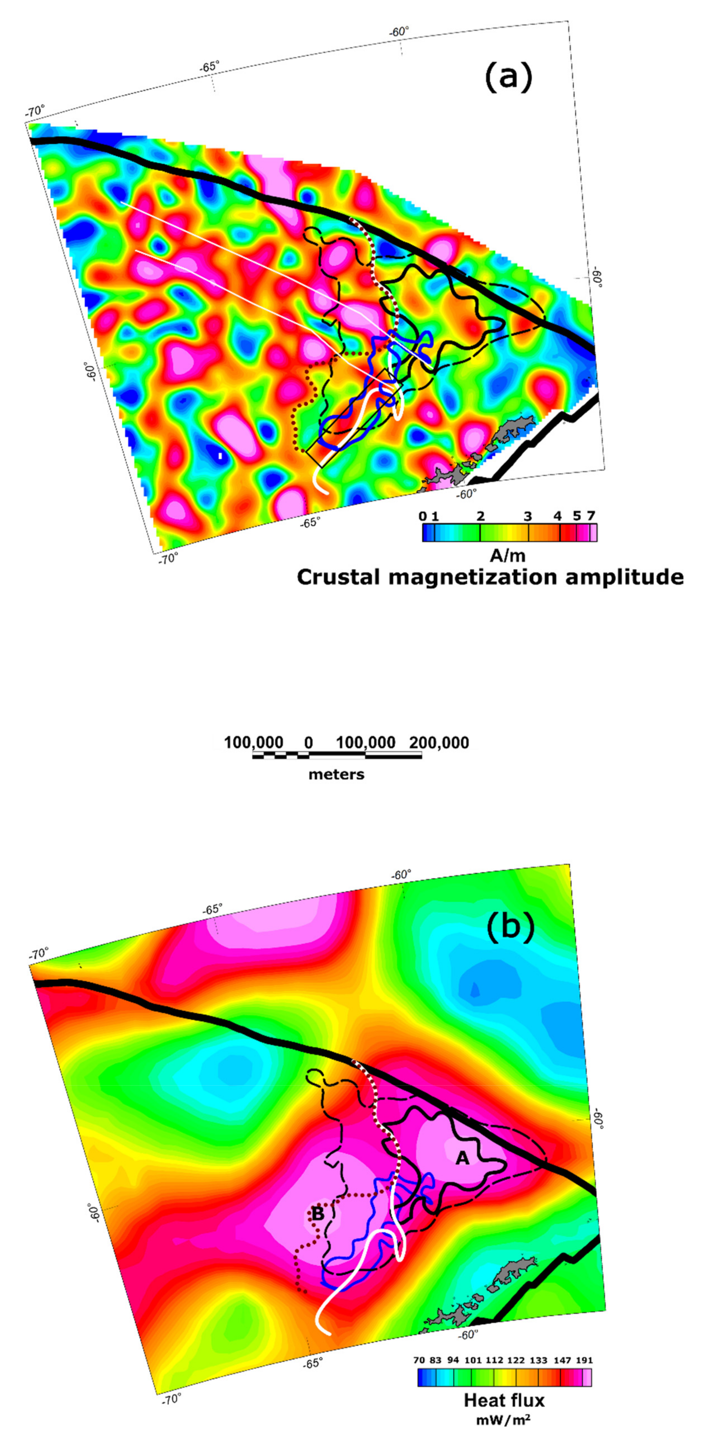
A third scenario to explain the decrease in magnetization is related to the age of the oceanic crust. This decay is widely accepted for young oceanic crust (<20 Ma), and it is attributed to low-temperature oxidation which affects the most extrusive rocks. This way, the titanomagnetite transforms into titanomaghemite, which is less magnetic. This decrease is very quick and intense close to the spreading ridge and during the beginning of the expansion (the first 4 My). Thereafter, the transformation process becomes slower, reaching equilibrium, or, even, the magnetization exhibits a slight increase [16,37]. In the case of the Phoenix Plate, the decrease in magnetization before and after crossing the boundary (Figure 5b and Figure 7a: thick solid black and white lines, respectively) is between 30% and 50%. This is not a gradual change, and it is much higher than expected for an oceanic crust of 7 My older than the one located at the ridge for the case of corridor P1 [9].

(iv)

Another option to explain the decrease in magnetization is a temporal variation of chemical properties of the magnetic minerals in the basalts that form the extrusive part of the oceanic crust along the oceanic corridors [38]. Prevot and Lecaille [39] showed differences in the smallest grain size of the magnetic minerals in the axial basalts with respect to the more remote basalts. This fact can explain local contrasts (areas of several kilometers), but it is does not seem feasible since the change in magnetization pattern is not constant for the same ages in the corridors and it is not present at both sides of the spreading axis.

None of the scenarios described above can explain the decrease in magnetization and the contrast observed between areas N and S (Figure 5b). Considering the four scenarios and arguments above, together with the fact that the decrease in magnetization varies from corridors P3 to P1 smoothly, with P1 being the higher affected area, we suggest that the decrease in magnetization is related to a process other than oceanic spreading.

The area where the decrease in the amplitude of magnetization starts agrees with the dashed black line which encloses the Bouguer gravity anomaly high (Figure 7a), mostly in the area where the highest values of Bouguer anomalies are found (thick black solid line). It is worth highlighting that in the southwestern-most area, this dashed black line coincides reasonably well with the inner part of the flexural bulge location (blue line).

Martos et al. [40] provided a map of geothermal heat flow (GHF) of the Scotia Arc. This map was obtained from magnetic anomaly data after applying spectral procedures. It shows the presence of high GHF values located along the boundaries of the Scotia Arc. This distribution was interpreted in terms of asthenospheric currents. One of the branches runs south of the southernmost tip of South America, while the other one runs north of the South Shetland archipelago. It was proposed that this asthenospheric current was established after the formation of the Shackleton Fracture Zone (middle to upper Miocene) [1,41,42], and it would have acted as a barrier for the asthenospheric flow through its lithospheric root, forcing the asthenospheric flow to divert and flow through lithospheric gaps: south of the southernmost tip of South America, and north of the South Shetland archipelago. Figure 7b shows the GHF map from [40] for the Phoenix Plate area. The map shows a high heat flow region with two main highs: one located NE and labeled as “A”, and another at the SW and labeled as “B”. A reasonable correlation exists between the Bouguer gravity anomaly high (highlighted within a thick black solid polygon in Figure 7b) and one of the two highs of GHF (Figure 7b: labeled as “A”) determined by [40].

In addition, Martos et al. [42] detected a rising of the mantle and a sharp lithospheric root in the proximity of the SFZ based on satellite gravity data. Vuan et al. [43] performed a reappraisal of surface wave tomography in the Scotia Sea region and surrounding areas. They used local and regional earthquakes recorded at permanent Antarctic stations from 2001 to 2013 and used them to update the measurements reported in [44]. Their Love group velocity tomographic maps at 25–30 s [43] (their Figure 10) shows a heterogeneity (a narrowing) in the group velocity anomalies maps with respect to the whole Scotia Sea area, which joins South America and the South Shetland archipelago. They show negative group velocity anomalies in this zone. This intermediate period (25–30 s) is controlled by crustal thickness and magmatic activities. The CRUST 1.0 model shows quite uniform crustal thickness for the entire Phoenix Plate, ranging from 6.8 km to 7.5 km. Considering this, we support a deep magmatic origin for these negative group velocities.

We propose that in the southeastern corner of the Phoenix Plate, the asthenospheric flow intersects the west flank of the SFZ and the flow piles up looking for a way to flow. This fact makes the heat flux to increase and therefore causes the Curie depth to reach shallower depths, which in turn affects the amplitude of the crustal magnetization due to thermal effects.

The second GHF high (Figure 7b: labeled as “B”) leads us to propose that the boundary inside the Phoenix Plate, setting the subarea where the amplitude of magnetization systematically decreases (Figure 7a: thin white line), should be extended further northwestward. In this way, we have included in Figure 7a a new thick dotted brown line highlighting the new boundary.

In Figure 7a, a rectangle marks an area of high magnetization. This is an unexpected feature as this local enhancement of the magnetization is found to the south of the boundary of the area where the magnetization decreases to a third of its value due to thermal causes.

As was mentioned before, the magnetic signature of the oceanic crust is produced by two layers: extrusive basalts (layer 2), and a second layer (layer 3) formed by gabbros, dolerites, and, in some cases, serpentinized peridotites. Although both layers contribute to the magnetic response, the shallowest layer (layer 2) is responsible for the seafloor magnetic anomalies. Extrusive basalts and gabbros have different Curie temperatures. Titanomagnetite is the main component of extrusive basalts and its Curie temperature ranges between 100–550 °C depending on the degree of oxidation [45], while for magnetite (which is the main component of gabbros), it is 580 °C [12].

The flexural bulge created by the subduction process is in the area highlighted in Figure 7a,b (as the blue solid line). An amplitude of magnetization of 5 A/m characterized this area, which represents an almost 2.5-fold reinforcement of the amplitude of magnetization with respect to the area immediately located northwestward. Taking into account an average GHF value in the area equal to 140 mW/m² and using an average value for the conductivity of 3.138 W/mK for the lithosphere [40], we can estimate the temperature range from the base of the crust to the upper limit of the lower crust, assuming a thickness of 5 km (values for the Moho depth and lower crust’s thickness according to the CRUST 1.0 model [29]). Proceeding this way, temperatures range from 367 °C (top of the lower crust) to 530 °C (for the Moho). In both cases, the temperature is lower than the Curie temperature for gabbro.

Seismic experiments carried out in the outer rise-trench region offshore of Costa Rica show bending-related faulting [46]. In these experiments, they detected active faulting which penetrates at least 20 km into the plate. Accordingly, they inferred that it provides a mechanism for pervasive infiltration of water into the crust and mantle. Contreras-Reyes et al. [47] obtained P-wave and S-wave velocity models using 2D travel time tomography off southern central Chile. They found variability in the Poisson’s ratio when comparing the top of the crust with the interface between layers 2 and 3, and the lowermost crust with the uppermost mantle. These features were interpreted as due to a highly weathered, altered and fractured oceanic crust. Ivandic et al. [48] obtained evidence showing alterations in the seismic properties of the subducting lithosphere using two seismic profiles running parallel to the Middle American Trench axis offshore of central Nicaragua. These results would support the serpentinization of the first 3 km of the upper mantle up to 24%.

We propose that the entire oceanic crust in the area, delimited by a thick dotted brown line (Figure 7a), is affected by a thermal anomaly caused by the asthenospheric supply. This causes a loss of almost threefold magnetization in this area. In addition, the flexural bulge causes the re-opening of old crustal cracks originally created at the ridge and new ones created by the bending-related faulting, producing a large population of cracks at lower crustal depths. These faults reaching to the lower crust would allow fluid to flow and alter gabbros and other magnetic minerals present in the crust. This alteration might enhance induced magnetization if gabbros are serpentinized, causing the increase in magnetization (Figure 7a).

5. Conclusions

In this study, we carried out an integrated geophysical study of the Phoenix Plate using magnetic anomalies, complete Bouguer gravity anomalies, and bathymetry. We derived a magnetization map that reveals the presence of NW–SE and NE–SW alignments (Figure 5a). The former occurs at the boundaries of the plate segments, P1–P2 and P2–P3, and presents a normal polarity. Following Tivey and Tucholke [16], we attribute these alignments to induced magnetism. This would explain a local reinforcement of the amplitude of magnetization that appears in the SW of the study area (Figure 7a: delimited by a rectangle). In this interpretation, NE–SW orientations would correlate with seafloor magnetic anomalies. In the short wavelength magnetization map (Figure 7b), two areas are clearly displayed: one in the northern part of the plate and one in the southern part. They present high magnetization values, while the area located southward shows a weakening in the amplitude of the magnetization. The amplitude of magnetization falls to almost a third of the values in the northern zone. It correlates to two other factors: (a) presence of an area where the Bouguer gravity anomalies reach the highest values in the whole study area, and (b) a heat flow branch that runs north of the South Shetland archipelago. These facts lead us to support past and present heat injection of the Pacific mantle outflow (as the heat flow branch may be still present) in the magnetization signature of the basin. Additionally, we identify a strong magnetization at the flexural bulge, possibly caused by reactivation of faults and generation of new bending faults. These faults, reaching into the lower crust, would allow fluid to flow and alter gabbros and other magnetic minerals present in the crust.

References

1. Livermore, R.; Eagles, G.; Morris, P.; Maldonado, A. Shackleton Fracture Zone: No barrier to early circumpolar ocean circulation. Geology 2004, 32, 797–800. [Google Scholar] [CrossRef] [Green Version]
2. Garrett, S.W.; Storey, B.C. Lithospheric Extension on the Antarctic Peninsula during Cenozoic Subduction. In Continental Extension Tectonics; Coward, M.P., Dewey, J.F., Hancock, P.L., Eds.; Geological Society, Special Publications: London, UK, 1987; Volume 28, pp. 419–431. [Google Scholar]
3. Larter, R.D.; Barker, P.F. Effects of ridge crest-trench interaction on Antartic-Phoenix spreading: Forced on a young subducting Plate. J. Geophys. Res. 1991, 96, 19583–19607. [Google Scholar] [CrossRef]
4. Cande, S.C.; Herron, E.M.; Hall, B.R. The early Cenozoic tectonic history of the southeast Pacific. Earth Planet. Sci. Lett. 1982, 57, 63–74. [Google Scholar] [CrossRef]
5. Livermore, R.; Balanyá, J.C.; Maldonado, A.; Martinez, J.M.; Rodriguez-Fernandez, J.; Sanz de Galdeano, C.; Galindo Zaldivar, J.; Jabaloy, A.; Barnolas, A.; Somoza, L.; et al. Autopsy on a dead spreading center: The Phoenix ridge, Drake Passage, Antarctica. Geology 2000, 28, 607–610. [Google Scholar] [CrossRef] [Green Version]
6. Jones, M.; Sandwell, D.; Beaman, R. New Soundings for SRTM30_Plusv7.0. In Proceedings of the Fifth Annual GEBCO Bathymetric Science Day, Callao, Peru, 15 September 2010; IHO/IOC Committee for the General Bathymetric Charts of the Ocean (GEBCO): Callao, Peru, 2010. [Google Scholar]
7. Bohoyo, F.; Larter, R.D.; Galindo-Zaldívar, J.; Leat, P.T.; Maldonado, A.; Tate, A.J.; Flexas, M.M.; Gowland, E.J.M.; Arndt, J.E.; Dorschel, B.; et al. Morphological and geological features of Drake Passage, Antarctica, from a new digital bathymetric model. J. Maps 2019, 15, 49–59. [Google Scholar] [CrossRef] [Green Version]
8. Maldonado, A.; Larter, R.D.; Aldaya, F. Forearc tectonic evolution of the South Shetland margin, Antartic Peninsula. Tectonics 1994, 13, 1345–1370. [Google Scholar] [CrossRef]
9. Eagles, G. Tectonic evolution of the Antarctic-Phoenix plate system since 15 Ma. Earth Planet. Sci. Lett. 2003, 217, 97–109. [Google Scholar] [CrossRef] [Green Version]
10. Jin, Y.K.; Kim, K.J.; Hong, J.K.; Park, M.; Nam, S.H.; Lee, J.H.; Kim, Y.D. Geophysical Investigations of P3 Segment of the Phoenix Ridge in Drake Passage, Antarctica, in Antarctica: A Keystone in a Changing World-Online. In Proceedings of the 10th ISAES X, Santa Barbara, CA, USA, 26 August–1 September 2007; Cooper, A.K., Raymond, C.R., Eds.; National Academies Press: Washington, DC, USA, 2007; Volume 4. [Google Scholar]
11. Nuñez Demarco, P.; Prezzi, C.; Sanchez Bettucci, L. Review of Curie point depth determination through different spectral methods applied to magnetic data. Geophys. J. Int. 2021, 224, 17–39. [Google Scholar] [CrossRef]
12. Dunlop, D.J.; Özdemir, Ö. Rock Magnetism: Fundamentals and Frontiers; Cambridge University Press: Cambridge, UK, 1997; 573p. [Google Scholar]
13. Chiozzi, P.; Matsuschima, J.; Okubo, Y.; Pasquale, V.; Verdoya, M. Curie point depth form spectral analysis of magnetic data in central-southern Europe. Phys. Earth Planet. Inter. 2005, 152, 267–276. [Google Scholar] [CrossRef]
14. Eppelbaum, L.V.; Pilchin, A.N. Methodolgy of Curie discontinuity map development for regions with low thermal characteristics: An example from Israel. Earth Planet. Sci. Lett. 2006, 243, 536–551. [Google Scholar] [CrossRef]
15. Tivey, M.; Johnson, H.P. Crustal magnetization reveals subsurface structure of Juan de Fuca Ridge hydrothermal vent fields. Geology 2002, 30, 979–982. [Google Scholar] [CrossRef]
16. Tivey, M.; Tucholke, B.E. Magnetization of 0–29 Ma ocean crust on the Mid-Atlantic Ridge, 25°30′ to 27°10′ N. J. Geophys. Res. 1998, 103, 17807–17826. [Google Scholar] [CrossRef] [Green Version]
17. Choe, H.; Dyment, J. Decreasing magnetization, lithospheric flexure and rejuvenated hydrothermalism off the Japan-Kuril subduction zone. Geophys. Res. Lett. 2020, 47, 1–7. [Google Scholar] [CrossRef]
18. Choe, H.; Dyment, J. The fate of marine magnetic anomaly in subduction zones: A global appraisal. Earth Planet. Sci. Lett. 2021, 561, 116787. [Google Scholar] [CrossRef]
19. Quesnel, Y.; Catalán, M.; Ishihara, T. A new global marine magnetic anomaly data set. J. Geophys. Res. 2009, 114, B04106. [Google Scholar] [CrossRef]
20. Catalán, M.; Dyment, J.; Choi, Y.; Hamoudi, M.; Lesur, V.; Thebault, E.; de Santis, A.; Ishihara, T.; Korhonen, J.; Litvinova, T.; et al. Making a better magnetic map. Eos 2016, 97, 1–9. [Google Scholar] [CrossRef]
21. Lesur, V.; Hamoudi, M.; Choi, Y.; Dyment, J.; Thèbault, E. Building the second version of the World Digital Magnetic Anomaly Map (WDMAM). Earth Planets Space 2016, 68, 27. [Google Scholar] [CrossRef]
22. Sabaka, T.J.; Olsen, N.; Purucker, M.E. Extending comprehensive models of the Earth’s magnetic field with Oersted and CHAMP data. Geophys. J. Int. 2004, 159, 521–547. [Google Scholar] [CrossRef]
23. Thébault, E.; Finlay, C.C.; Beggan, C.; Alken, P.; Aubert, J.; Barrois, O.; Bertrand, F.; Bondar, T.; Boness, A.; Brocco, L.; et al. International Geomagnetic Reference Field: The 12th generation. Earth Planet. Space 2015, 67, 79. [Google Scholar] [CrossRef]
24. Kuhn, M.; Featherstone, W.E.; Kirby, J.F. Complete spherical Bouguer gravity anomalies over Australia. Aust. J. Earth Sci. Int. Geosci. J. Geol. Soc. Aust. 2009, 56, 213–223. [Google Scholar] [CrossRef]
25. Bonvalot, S.; Balmino, G.; Briais, A.; Kuhn, M.; Peyrefitte, A.; Vales, N.; Biancale, R.; Gabalda, G.; Reinquin, F.; Sarrailh, M. World Gravity Map; Commission for the Geological Map of the World, Ed.; BGI-CGMW-CNES-IRD: Paris, France, 2012. [Google Scholar]
26. Pavlis, N.K.; Holmes, S.A.; Kenyon, S.C.; Factor, J.K. An Earth Gravitational Model to degree 2160: EGM2008. In Proceedings of the General Assembly of the European Geosciences Union, Vienna, Austria, 13–18 April 2008. [Google Scholar]
27. Balmino, G.; Vales, N.; Bonvalot, S.; Briais, A. Spherical harmonic modeling to ultra-high degree of Bouguer and isostatic anomalies. J. Geod. 2012, 86, 499–520. [Google Scholar] [CrossRef]
28. Amante, C.; Eakins, B.W. ETOPO1 1 Arc-Minute Global Relief Model: Procedures, Data Sources and Analysis. In NOAA Technical Memorandum NESDIS NGDC-24; National Geophysical Data Center Marine Geology and Geophysics Division: Boulder, CO, USA, 2009. [Google Scholar]
29. Laske, G.; Masters, G.; Ma, Z.; Pasyanos, M. Update on CRUST1.0—A 1-degree Global Model of Earth’s crust. Geophys. Res. Abstr. 2013, 15, 2658. [Google Scholar]
30. Parker, R.L.; Huestis, S.P. The inversion of magnetic anomalies in the presence of topography. J. Geophys. Res. 1974, 79, 1587–1593. [Google Scholar] [CrossRef]
31. Garrett, S.W. Interpretation of reconnaissance gravity and aeromagnetic surveys of the Antartic Peninsula. J. Geophys. Res. 1990, 95, 6759–6777. [Google Scholar] [CrossRef]
32. Ghidella, M.E.; Yánez, G.; LaBreque, J.L. Revised tectonic implications for the magnetic anomalies of the western Weddell Sea. Tectonophysics 2002, 347, 65–86. [Google Scholar] [CrossRef]
33. Suriñach, E.; Galindo-Zaldívar, J.; Maldonado, A.; Livermore, R. Large amplitude magnetic anomalies in the northern sector of the Powell Basin, NE Antarctic Peninsula. Mar. Geophys. Res. 1997, 19, 65–80. [Google Scholar]
34. Hayes, G.P.; Wald, D.J.; Johnson, R.L. Slab1.0: A three-dimensional model of global subduction zone geometries. J. Geophys. Res. Solid Earth 2012, 117, 1–15. [Google Scholar] [CrossRef]
35. Johnson, P.H.; Pruis, M.J.; Van Patten, D.; Tivey, M.A. Density and porosity of the upper oceanic crust from seafloor gravity measurements. Geophys. Res. Lett. 2000, 27, 1053–1056. [Google Scholar] [CrossRef] [Green Version]
36. Juárez, M.T.; Tauxe, L.; Gee, J.S.; Pick, T. The intensity of the Earth’s magnetic field over the past 160million years. Nature 1998, 394, 878–881. [Google Scholar] [CrossRef] [Green Version]
37. Pockalny, R.A.; Smith, A.; Gente, P. Spatial and temporal variability of crustal magnetization of a slowly spreading ridge: Mid_Atlantic Ridge (20°–24° N). Mar. Geophys. Res. 1995, 17, 301–320. [Google Scholar] [CrossRef]
38. Tivey, M.A.; Johnson, H.P. The Central Anomaly high: Implications for ocean crust construction and evolution. J. Geophys. Res. 1987, 92, 12685–12694. [Google Scholar] [CrossRef]
39. Prevot, M.; Lecaille, A. Comments on paper by Klitgord, K.D. Sea-floor spreading: The central anomaly Magnetization High. Earth Planet. Sci. Lett. 1976, 33, 164–168. [Google Scholar] [CrossRef]
40. Martos, Y.M.; Catalán, M.; Galindo-Zaldívar, J. Curie depth, heat flux and thermal subsidence studies reveal the Pacific mantle outflow through the Scotia Sea. J. Geophys. Res. Solid Earth 2019, 124, 10735–10751. [Google Scholar] [CrossRef]
41. Martos, Y.M.; Maldonado, A.; Lobo, F.J.; Hernández-Molina, F.J.; Pérez, L.F. Tectonics and palaeoceanographic evolution recorded by contourite features in southern Drake Passage (Antarctica). Mar. Geol. 2013, 343, 76–91. [Google Scholar] [CrossRef]
42. Martos, Y.M.; Galindo-Zaldívar, J.; Catalán, M.; Bohoyo, F.; Maldonado, A. Asthenospheric Pacific–Atlantic flow barriers and the west Scotia ridge extinction. Geophys. Res. Lett. 2014, 41, 1–7. [Google Scholar] [CrossRef]
43. Vuan, A.; Sugan, M.; Plasencia Linares, M.P. Reappraisal of surface wave group velocity tomography in the Subantarctic Scotia Sea and surrounding ridges. Glob. Planet. Chang. 2014, 123, 223–238. [Google Scholar] [CrossRef]
44. Vuan, A.; Russi, M.; Panza, G.F. Group velocity tomography in the sub-antarctic Scotia Sea region. Pure Appl. Geophys. 2000, 157, 1337–1357. [Google Scholar] [CrossRef]
45. Zhou, W.; Van der Voo, R.; Peacor, D.R.; Wang, D.; Zhang, Y. Low-temperature oxidation in MORB of titanomagnetite to titanomaghemite: A gradual process with implications for marine magnetic anomaly amplitudes. J. Geophys. Res. 2001, 106, 6409–6421. [Google Scholar] [CrossRef]
46. Ranero, C.R.; Phipps Morgan, J.; McIntosh, K.; Reichert, C. Bending-related faulting and mantle serpentinization at the Middle America trench. Nature 2003, 425, 367–373. [Google Scholar] [CrossRef]
47. Contreras-Reyes, E.; Grevemeyer, I.; Flueh, E.R.; Scherwath, M.; Bialas, J. Effect of trench-outer rise bending-related faulting on seismic Poisson’s ratio and mantle anisotropy: A case study offshore of Southern Central Chile. J. Geophys. J. Int. 2008, 173, 142–156. [Google Scholar] [CrossRef] [Green Version]
48. Ivandic, M.; Grevemeyer, I.; Bialas, J.; Petersen, C.J. Serpentinization in the trench-outer rise region offshore of Nicaragua: Constraints from seismic fraction and wide-angle data. Geophys. J. Int. 2010, 180, 1253–1264. [Google Scholar] [CrossRef] [Green Version]
Figure 2. Magnetic anomaly map. Two solid curvilinear polygons encircle the areas where the largest amplitude of magnetic anomalies is located. Plate boundaries are represented by black solid thick lines. SSMA: South Shetlands magnetic anomaly. P1, P2, and P3 denote the three inactive plate segments of the Phoenix Ridge. Two black thin dotted lines separate P1, P2, and P3 zones. HFZ: Hero Fracture Zone. SFZ: Shackleton Fracture Zone. Both fracture zones are depicted with thick and thin black lines, respectively.
Remotesensing 14 01642 g002
Figure 3. Complete Bouguer gravity anomaly map. Plate boundaries are represented by black solid thick lines. A black solid polygon denotes the location of a triangular high anomaly area, and a white curvilinear polygon denotes the area where highest values of Bouguer anomalies are found. P1, P2, and P3 denote the three inactive plate segments of the Phoenix Ridge and are located over their respective ridges. Two black thin dotted lines separate P1, P2, and P3 zones. HFZ: Hero Fracture Zone. SFZ: Shackleton Fracture Zone. Both fracture zones are depicted with thick and thin black lines, respectively.
Remotesensing 14 01642 g003
Figure 4. Sediment thickness map of the study area. Contour lines every 250 m. Plate boundaries are denoted by black solid thick lines.
Remotesensing 14 01642 g004
Figure 5. (a) Crustal magnetization map obtained after a bandpass filter with long and short wavelength cutoffs of 200 km and 7 km. Two thick black dotted lines denote the Shackleton Fracture Zone (SFZ) and the Hero Fracture Zone (HFZ). Two white solid lines separate P1, P2, and P3 zones. R1, R2, and R3: ridges locations. Thin black dotted lines perpendicular to P1, P2, and P3 denote the location of the central normal polarity segments according to [5,9,10]. C4 and C5: Chrons of seafloor spreading magnetic anomalies. The white dotted ellipse denotes a normal magnetization alignment (see text for details). Black solid polygon indicates NW–SE alignment (see text for details). Black dotted polygon indicates positive magnetization area (see text for details). The magnetization of the South Shetland archipelago block is marked with a black dashed-dotted polygon. (b) Crustal magnetization map obtained after a bandpass filter with long and short wavelength cutoffs of 100 km and 7 km, respectively. Black line delimits two areas labeled as N and S (see text for comments). Both areas differ in orientation and in amplitude of the magnetization signals. Plate boundaries are denoted by black solid thick lines.
Remotesensing 14 01642 g005aRemotesensing 14 01642 g005b
Figure 6. Radial average spectrum applied on the area located north (in blue) of the black continuous line (Figure 5b) and south (in black) of it.
Remotesensing 14 01642 g006
Figure 7. (a) Spatial variation of the magnetization pattern. Two white solid lines separate plate segments P1, P2, and P3. (b) The figure shows the heat flux map from Martos et al. (2019). Letters “A” and “B” denote two heat flux maxima. A brown curvilinear dotted line denotes the new boundary depicting where magnetization decreases, while a thick solid white line denotes the proposed magnetization boundary in Figure 5b. A rectangle (only in Figure 7a) denotes an area where magnetization increases (see text for comments). A thin black dashed polygon denotes the location of a triangular Bouguer maxima anomaly area, and a thick black solid polygon denotes the area where highest values are reached within this section. A blue solid line denotes the location of the flexural bulge.
Remotesensing 14 01642 g007
Publisher’s Note: MDPI stays neutral with regard to jurisdictional claims in published maps and institutional affiliations.