Abstract
Anthropogenically-driven climate change, land-use changes, and related biodiversity losses are threatening the capability of forests to provide a variety of valuable ecosystem services. The magnitude and diversity of these services are governed by tree species richness and structural complexity as essential regulators of forest biodiversity. Sound conservation and sustainable management strategies rely on information from biodiversity indicators that is conventionally derived by field-based, periodical inventory campaigns. However, these data are usually site-specific and not spatially explicit, hampering their use for large-scale monitoring applications. Therefore, the main objective of our study was to build a robust method for spatially explicit modeling of biodiversity variables across temperate forest types using open-access satellite data and deep learning models. Field data were obtained from the Biodiversity Exploratories, a research infrastructure platform that supports ecological research in Germany. A total of 150 forest plots were sampled between 2014 and 2018, covering a broad range of environmental and forest management gradients across Germany. From field data, we derived key indicators of tree species diversity (Shannon Wiener Index) and structural heterogeneity (standard deviation of tree diameter) as proxies of forest biodiversity. Deep neural networks were used to predict the selected biodiversity variables based on Sentinel-1 and Sentinel-2 images from 2017. Predictions of tree diameter variation achieved good accuracy (r2 = 0.51) using Sentinel-1 winter-based backscatter data. The best models of species diversity used a set of Sentinel-1 and Sentinel-2 features but achieved lower accuracies (r2 = 0.25). Our results demonstrate the potential of deep learning and satellite remote sensing to predict forest parameters across a broad range of environmental and management gradients at the landscape scale, in contrast to most studies that focus on very homogeneous settings. These highly generalizable and spatially continuous models can be used for monitoring ecosystem status and functions, contributing to sustainable management practices, and answering complex ecological questions.
1. Introduction
Forests cover about 31 percent of the global land surface and provide a variety of valuable ecosystem services. By taking up large amounts of atmospheric carbon, forests act as important climate regulators; they provide habitat for the majority of terrestrial biodiversity and hold high cultural and aesthetic values. However, forests face tremendous challenges under climate change, deforestation, increasing disturbances, and declining biodiversity [1]. Biodiversity is known to be a key determinant of the capability of forests to maintain their ecosystem functioning against these impacts [2]. Quantitative information on the state and changes of forest biodiversity is critical for sustainable management and conservation goals [3]. To harmonize global efforts on biodiversity monitoring, the Group on Earth Observations Biodiversity Observation Network (GEO BON) established the framework of essential biodiversity variables (EBVs). It is based on a minimum set of measurable indicators that cover a broad range of biodiversity components, such as genetic composition, ecosystem structure, and ecosystem function [4]. The potential of Earth Observation (EO) data for the global monitoring of EBVs has been recently emphasized by Skidmore et al. [5]. Satellite remote sensing techniques allow the derivation of ecologically meaningful information and represent a valuable tool for continuous, large-scale monitoring applications that are still to be operationally implemented in forest research and management at national scales, e.g., in Germany [6]. However, modeling biodiversity from satellite images remains a huge challenge; used data and methods differ across scientists and study areas, and a generic, robust approach is still lacking [7,8].
Multiple studies have addressed the need for a more thorough understanding of the relationships between plant diversity and spectral information derived from remote sensing imagery [9,10]. Common approaches use plot-based spectral band data and vegetation indices from optical data, such as provided by Sentinel-2 or Landsat, to model in situ plant diversity indices in Mediterranean forests [10,11], mountainous forests [12,13], and subtropical forests [14]. Fagua et al. [15] revealed strong relationships between backscatter variables computed from Sentinel-1 radar data and tree species diversity in tropical forests, while another study showed moderate correlations with structural parameters (tree height and fractional cover) in temperate deciduous forests [16]. To provide more meaningful insights into the relationship between plant diversity and the remote sensing signal, an increasing number of studies have made use of the spectral variation hypothesis [9,13,17,18]. The capability of Rao’s Q index, a measure of spectral abundance and distance, to capture vegetation heterogeneity from satellite images has been presented in [19]. Nonetheless, in the case of forests, Rao’s Q index has only been experimentally tested without incorporating heterogeneous forest data [13,20].
Other researchers have switched the focus from species diversity to functional diversity, which is understood as the range, abundance, and distribution of species traits, such as structural diversity [21]. Spatially variable environments facilitate resource partitioning and resilience against disturbances, linking species diversity with ecosystem functions [21]. There are different measures for stand structural attributes that describe the complexity of stand structure. Measures that emerged from growth and yield sciences address the stand density, size distribution, stand age composition as well as the horizontal and vertical arrangement of trees. For size distributions, statistical metrics such as the standard deviation of tree diameter or basal area are used [22]. On the other side, there are other approaches that integrate multiple stand structural attributes into a single index to more adequately address the three-dimensional characteristics of forest structure, e.g., Storch et al. [23].
Recent research has highlighted strong relationships between forest structural diversity and tree species diversity [24], or bird diversity [25], at the global scale. Thus, models of overstorey and canopy structure using remote sensing data have recently become more common in forest biodiversity mapping [16,26]. Such approaches typically rely on active remote sensing, either acquired by airborne laser scanning (ALS) [27] or spaceborne synthetic aperture radar (SAR) systems [28]. However, multiple studies also indicated the potential of features computed from optical data to model structural diversity variables [27,29,30]. The usage of spatial texture features as a measure of vegetation heterogeneity that is being computed from spectral bands and/or vegetation indices tends to be promising for enhancing spatial models of plant diversity, but the evidence is still scarce [29,31].
As indices of tree species diversity and structural attributes of forests represent continuous data, statistical regression models are used for such analysis. Most prevalent are machine learning (ML) models such as random forest (RF) [8,10,12,32]. Only a very few studies used deep learning (DL) models for similar tasks [30], though their application for biodiversity modeling with remote sensing data is very promising and thus should be tested. In such studies, the validation of regression models is usually performed by calculating a set of accuracy metrics such as the root mean squared error (RMSE) or the coefficient of determination (r2). Reported r2 of tree species diversity models ranged between 0.3 and 0.7 [11,13], while according to [8,33], the relative root mean squared error (RRMSE) ranged between 20% and 38% for tree diameter and 13% to 30% for tree height.
Reviewing previous research, we identified several knowledge gaps in the field of the spatial modeling of forest biodiversity variables. So far, published studies that use ML models and remote sensing data, e.g., [8,11], have addressed single components of forest structure, either referring to species composition or growing stock. In general, the application of DL to both optical and radar imagery for biodiversity modeling requires more research. Another research gap in current literature is the lack of analysis that tests the transferability of published models across heterogeneous forest types and management intensities. The often-limited availability of field data results in case-specific models [8,13,28]. Considering these research gaps, the detailed objectives of our study were
- To build and test a consistent modeling method for predicting different facets of forest structure relevant to biodiversity research and forest management planning.
- To examine the predictive power of DL models for different types of predictors extracted from radar and optical image data.
- To produce spatially explicit DL models that can generalize forest structural attributes across temperate forest types.
In our approach, we consolidated recent findings revealing predictable relationships between spectral image features and in situ forest variables. We employed a complete dataset containing a broad diversity of forest types across Germany to develop a model that can generalize forest structural attributes across forest types and thus, address the research gap related to the model’s transferability.
2. Materials and Methods
2.1. Study Sites
The study was conducted throughout the three Biodiversity Exploratories (BE) that are distributed across Germany, following topographic and climatic gradients, and represent the variety of temperate forest types. Table 1 shows general geographical information of the study sites; a map showing the locations of the study sites is given in Figure 1.

Table 1.
Characteristics of the three study sites, modified from [34].
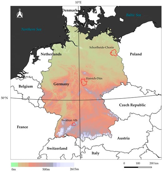
Figure 1.
Locations of the three study sites across Germany. The background image shows the topographic gradient based on NASA Shuttle Radar Topography Mission (SRTM) data.
2.1.1. Schorfheide-Chorin
Schorfheide-Chorin is embedded in an undulating moraine landscape in north-eastern Germany. Figure 2 shows the spatial distribution of forest types within the study area. The 1300 km2 big UNESCO biosphere reserve is located within one of the driest regions of Germany, dominated by extensive pine forests that grow on alluvial quartz sands upon the Pleistocene ground moraine accounting for 67% of the area. Another 28%, where the ground moraine surfaces, are covered by deciduous forests [35].
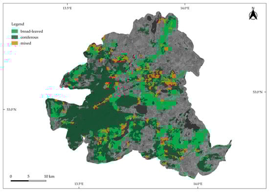
Figure 2.
Location of the study site Schorfheide-Chorin. Forest type cover information was taken from the Corine Land Cover Dataset 2018 (© European Union, Copernicus Land Monitoring Service 2021, European Environment Agency).
2.1.2. Hainich-Dün
The National park Hainich, with a size of about 1300 km2, is located in northern Thuringia in central Germany. The regional climate is more humid here than in Schorfheide-Chorin due to the crossing of a low mountain ridge. Forests grow on limestone bedrock, with deciduous forests covering 83% of the area [32]. Figure 3 gives an overview of the spatial distribution of forest types.
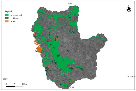
Figure 3.
Location of the study site Hainich-Dün. Forest type cover information was taken from the Corine Land Cover Dataset 2018 (© European Union, Copernicus Land Monitoring Service 2021, European Environment Agency).
2.1.3. Swabian Alb
The exploratory Swabian Alb is the smallest among the three study sites, with an area of about 430 km2. The low mountain range landscape exhibits a stronger topographic control with heights of up to 860 m a.s.l. Forests grow on limestone, and around 78% of the forest area can be classified as deciduous, including mixtures of Fagus and Picea [35]. Figure 4 shows a forest cover map of the study site.
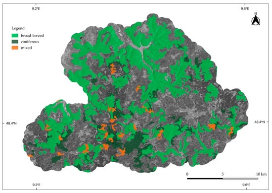
Figure 4.
Location of the study site Swabian Alb. Forest type cover information was taken from the Corine Land Cover Dataset 2018 (© European Union, Copernicus Land Monitoring Service 2021, European Environment Agency).
2.2. Data
2.2.1. Sampling Design
The collection of in situ data on forest structure variables drew on the network of field plots established by the BE project across the three study sites. From 500 grid plots of diverse forest areas, 150 forest plots (50 per exploratory) of 1 ha size were accounted as experimental plots (EPs) for more extensive research. The selection of EPs followed a stratified sampling design to cover the variation in soil depth and land-use intensities within each exploratory. During inventory surveys between 2014 and 2018, data on stand structure were sampled within the frame of the BE core project on forest structure. From single tree data, leaving out thickets with a diameter below 7 cm, a dataset on stand structural attributes was constructed by Schall et al. [36] and used in this study.
2.2.2. Forest Management Types
In general, the definition of management types within the study regions results from harvesting practices rather than specific structural characteristics [35]. Furthermore, forests within the exploratories were structurally shaped by diverse management practices rather than by species diversity which is relatively low across Central European forests [36]. Age-class forests are among the most extensive management type, being either dominated by Fagus sylvatica, Picea abis, or Pinus sylvestris. A few stands are dominated by Fraxinus excelsior and Acer pseudoplatanus. Plots in Schorfheide-Chorin cover Scots pine, European beech, pine/beech, and oak forests. Plots of pine forests show different development stages compared to other mature forest stands. Forest plots in Hainich-Dün are dominated by beech with different development stages as well as unmanaged and selection systems. In Swabian Alb, age-class beech forests of all development stages were selected, while the topographic conditions have favored extensive plantations of Norway spruce, of which immature stands were included [36]. In total, the inventory covered field data on 14 forest types according to management and dominating species.
2.2.3. Selection of Study Variables
Forest structure may be concisely defined as the spatial distribution of trees of different sizes and ages within a stand. A variety of characteristics exist to describe the different components of forest structure, such as species and age composition, stand density, and size distribution [36]. As derivatives of stand productivity, biodiversity, and ecosystem resilience, stand structural attributes provide valuable information for forest management authorities and ecologists [36]. For our study, we obtained quantitative, in situ data on species composition and size distribution as measures of forest structure.
Species composition encompasses the number of species and their frequency distribution within a stand [37]. Here, the Shannon Wiener diversity index was used as a proxy of tree species diversity that was calculated from tree species abundance data. This index is commonly gathered for estimating local alpha-diversity [36] as in similar studies before [13,17,18].
The determination of stand tree size distribution often includes the use of statistical descriptions of dendrometric state variables such as basal area, tree diameter, height, and volume [38]. In this study, the standard deviation of tree diameter at breast height (DBH) was selected as an indicator of tree size heterogeneity. Moreover, we applied our approach to other stand structural attributes, namely the standard deviation of tree height, basal area, and Reineke’s stand density index [36].
2.2.4. Selection of Predictors Extracted from Satellite Data
For this study, different types of satellite data have been gathered that were resampled to 10 m pixel resolution. Sentinel-1 data have majorly been used for modeling structural diversity and Sentinel-2 data for species diversity. However, also multi-sensor models have been produced for both study variables. As the field sampling took place between 2014 and 2018, so that the plots have been measured in different years, it was the most convenient to select 2017 as one common year in between for the acquisition of the satellite data. Moreover, 2017 was the year with the highest frequency of valid observations, being partly attributed to the launches of Sentinel-1 in 2016 and Sentinel-2B in 2017.
Sentinel-1 SAR acquisitions have been extracted from the collection provided in Google Earth Engine (GEE). This catalog includes ground range detection imagery that was preprocessed with the Sentinel-1 toolbox. Detailed information on the standardized preprocessing steps of Sentinel-1 SAR data can be found in [39]. Based on images from 2017 and the winter season 2017/2018, median backscatter composites have been produced for both polarizations (VH and VV) and both orbit paths (ascending and descending) separately for each study site. In addition, the normalized difference of both polarizations for the winter season has been computed. Then median backscatter values for the plot areas were extracted so that in the end, there were ten Sentinel-1 predictors, as shown in Table 2.
Table 2.
List of model predictors used according to the sensor and feature type and corresponding abbreviations.
In GEE, the ML algorithm s2cloudless [40] was implemented to create cloud and cloud shadow masked median Sentinel-2 composites for the growing season 2017 for each study site based on images from the surface reflectance collection provided in the GEE data catalog. This Level-2A product comes already atmospherically corrected and orthorectified. Optical data from the winter season were not included due to snow cover interferences and pronounced cloud contamination in the images. Median and standard deviation values of Enhanced Vegetation Index (EVI) composites were extracted in GEE. The EVI uses the red, blue, and NIR bands [29]:
and has been proven to be useful for dense canopy areas superior to other vegetation indexes such as the Normalized Vegetation Index (NDVI). An overview of the 12 predictors extracted from Sentinel-2 spectral band composites is given in Table 2.
Additional metrics were calculated that describe the spatial texture, or more specifically, the spatial distribution of reflectance intensities [41]. Multiple studies could make out relationships between the spatial texture in remote sensing images and habitat heterogeneity of grassland and forest ecosystems [29,42,43]. From the EVI and normalized difference of VV and VH backscatter [16], four texture features (contrast, homogeneity, entropy, dissimilarity) were calculated based on the Gray-Level-Co-Occurrence-Matrix (GLCM) using the function glcmTexture in GEE [29]. For this, a fixed window with a size of 3 × 3 pixels had to be specified. A description of the texture features is provided in Table 3.
Table 3.
Overview, description, and formula of applied textural metrics based on [29,41].
Spectral heterogeneity is another method to assess plant diversity patterns. Rao’s Q diversity index applied to satellite data was recently tested as a proxy of environmental heterogeneity. Rao’s Q index measures the regional abundance and spectral distance of pixel values [19]:
where dij is the spectral distance between pixels i and j and p the proportion of occupied area [19]. Studies revealed correlations with tree species diversity [13,18,44,45]. Rao’s Q index measures the regional abundance and spectral distance of pixel values [19]. We included the index to test for its application in predicting tree species and structural diversity. It was calculated in ArcGIS based on the ten Sentinel-2 bands using a 3 × 3 pixel kernel [44].
2.3. Deep Neural Network Regression
For biodiversity modeling, we implemented a feed-forward deep neural network (DNN) using Keras sequential model in Python. The architecture, together with the overall workflow of this study, is presented in Figure 5. The DNN was built with five layers: A normalization layer, an input layer with 64 neurons, two inner layers with 64 neurons each, and an output layer with one neuron. We chose the rectified linear unit (relu) as activation function, the optimizer RMSprop, and the mean absolute error as a loss function. The loss function achieved a stable minimum at 100 epochs. DNN architecture (number of layers and nodes) and hyper parameters were fine-tuned empirically by minimizing the root mean squared error in the training data. More information about the nature of these parameters is given in [46,47,48,49].
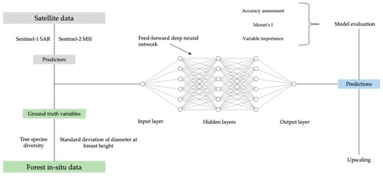
Figure 5.
Workflow and architecture of the deep neural network.
We based the validation of our models on a set of common accuracy metrics. The RMSE and RRMSE were used to assess the differences between in situ data and predictions. The latter is standardized by the mean of the validation observations. The coefficient of determination (r2) is the most commonly used metric for the validation of prediction models. It represents the proportion of variance of the response variable that has been explained by the model predictors. However, r2 alone is not sufficient to assess the performance of a model since it can not estimate bias. For the detection of bias, scatterplots of predictions versus in situ values were used in this study. Additionally, the RMSE and derivatives, such as the RRMSE, allowed the comparison of different models. Each model was run ten times while selecting training and validation data randomly each time. The average results, as well as their variation across the ten folds, were finally calculated.
To have a thorough understanding of the capabilities of our models, we also analyzed the predictor importance by a leave-one-out approach, separately for each feature group and each target variable. That type of approach leaves one predictor out with each iteration in order to evaluate the loss in accuracy when the said predictor is removed. Spatial autocorrelation was taken into account by calculating Moran’s I.
3. Results
In the following section, we will separately report on the model accuracies and predictor importance of the models of tree species diversity and tree diameter variation.
3.1. Tree Species Diversity
3.1.1. Predictors Importance
The importance of used model predictors is presented in Figure 6. We categorized all 31 predictors into four general feature groups: (i) Sentinel-2 spectral bands, Rao’s Q and EVI, (ii) Sentinel-1 backscatter features, and the normalized difference of winter VV and VH, which was found to be more useful for prediction than VV and VH data from the growing season, (iii) Sentinel-2 texture based on EVI and (iv) Sentinel-1 texture based on the normalized difference of winter VV and VH. For each of the models, we evaluated the individual contribution of features to the predictive performance. The standard deviation of EVI was the most relevant predictor within the Sentinel-2 group (i).
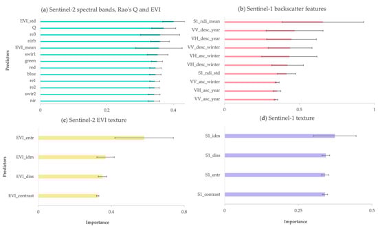
Figure 6.
Predictor importance for tree species diversity models for the four different feature groups (a–d). The error bars indicate the variation in importance across the ten folds where training and validation data have been randomized.
We observed no significant differences between Sentinel-2 multi-spectral bands. However, vegetation red edge and narrow NIR bands performed slightly better for tree species diversity. Rao’s Q index revealed the second highest importance. Regarding the second feature group (ii), the normalized difference of winter VV and VH showed the highest importance, followed by single-year VV and VH. The Sentinel-2 texture features (iii) showed a more distinct variability in importance compared to the Sentinel-1 texture features (iv). EVI-based entropy was by far the best predictor within the group of multi-spectral texture features.
3.1.2. Model Accuracies
Accuracies of tree species diversity models, summarized over ten iterations, are reported in Table 4 according to the feature group used. We trained and tested several models using different sets of predictors. The lowest RMSE and highest r2 were obtained when all 31 predictors were used. Texture metrics of EVI achieved the same RMSE, and differences in r2 were not significant.
Table 4.
Model accuracy metrics (root mean squared error, relative root mean squared error, coefficient of determination) of tree species diversity models. The table with heatmap (red = low accuracy, blue = high accuracy) shows the median and standard deviation values summarized over ten model iterations.
Overall, the models incorporating Sentinel-1 features tended to show lower accuracies. A scatterplot showing the correlation between predicted and in situ values of the best model for tree species diversity, which is based on EVI texture features, is presented in Figure 7.
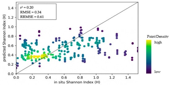
Figure 7.
Density scatterplot showing the relationship between predictions of tree species diversity (Shannon Wiener Index) and in situ values based on the EVI texture model.
The assessments of spatial autocorrelation revealed values of Moran’s I near zero, thus indicating low spatial dependency in our dataset, in the case of tree species diversity as a study variable shown in Table 5.
Table 5.
Moran’s I result for tree species diversity across the three exploratories. For z-score values between ± 1.65 random distribution of samples can be assumed.
3.2. Structural Diversity
3.2.1. Predictors Importance
Predictor importance for different models of the standard deviation of DBH is shown in Figure 8. For the model calibrated with Sentinel-2 multi-spectral band features, the NIR and red bands showed slightly higher importance than the other bands, whereas EVI and Rao’s Q were among the least important predictors contrary to the model of species diversity.
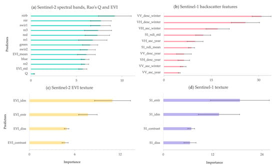
Figure 8.
Predictor importance for structural diversity models for the four different feature groups (a–d). The error bars indicate the variation in importance across the ten folds where training and validation data have been randomized.
Among the Sentinel-1 backscatter features, descending orbital winter VV and VH were significantly ranked higher than the other features in this group. Using dual-polarized VV backscatter, slightly higher accuracies for modeling structural diversity compared to VH were received. Among the Sentinel-2 texture features, the inverse difference moment (IDM) was ranked as most important, while for the Sentinel-1 texture features, entropy was ranked the highest.
3.2.2. Model Accuracies
Accuracy metrics for the models of structural diversity are listed in Table 6. For the standard deviation of the DBH, the lowest RMSE and highest r2 were returned when sixteen Sentinel-1 features were used. Adding all 31 predictors did not provide significantly higher accuracies in terms of RRMSE and r2.
Table 6.
Model accuracy metrics (root mean squared error, relative root mean squared error, coefficient of determination) of structural diversity models. The table with heatmap (red = low accuracy, blue = high accuracy) shows the median and standard deviation values summarized over ten model iterations.
Figure 9 shows the relationship between predicted values of the standard deviation of DBH and corresponding in situ values. Moran’s I and z-scores, documented in Table 7, suggest no occurrence of spatial autocorrelation, despite z-values being higher for models of Hainich-Dün and Schorfheide-Chorin, and the model including data from all study sites compared to the model of tree species diversity.
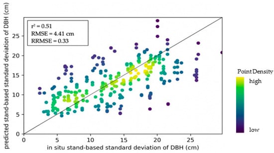
Figure 9.
Density scatterplot showing the relationship between predictions of structural diverstiy (standard deviation of DBH) and in situ values for 150 plots based on the model with sixteen Sentinel-1 features.
Table 7.
Moran’s I results for structural diversity across the three exploratories. For z-score values between ±1.65 random distribution of samples can be assumed.
3.3. Model Accuracies for Other Structural Variables
We applied the model of structural diversity to test the performance of our approach for other structural variables from the inventory: (i) standard deviation of tree height, (ii) tree basal area per hectare, (iii) tree density.
These variables have been modeled in previous studies that address remote sensing of forest structure and used ML models [8,30], whereas the basal area and tree density are rather variables associated with timber resources, and the distribution of tree heights is an important proxy of vertical layering and habitat heterogeneity [50]. Table 8 contains the achieved accuracies for the model using all features. Accuracies of tree height standard deviation were significantly lower compared to DBH standard deviation, whereas models of basal area and stand density achieved moderate accuracies. Figure 10 presents the comparisons of predictions versus in situ observations for the three structural attributes.
Table 8.
Model accuracy metrics of additional structural attributes extracted from the forest inventory. The structural diversity model comprising all 31 predictors has been used.
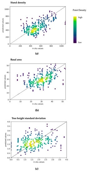
Figure 10.
Density scatterplots of (a) stand density index; (b) tree basal area (m); (c) tree height standard deviation (m). Predictions are based on the model that includes both Sentinel-1 and Sentinel-2 metrics.
3.4. Spatial Patterns of Predicted Tree Diameter Variation
Tree diameter variation was mapped for forested areas of all study sites using the simplest (i.e., least number of predictors) and best-performing model that included the Sentinel-1 entropy, VV, and VH backscatter features. The maps presented in Figure 11 and Figure 12 allow for visually assessing spatial patterns of structural diversity.
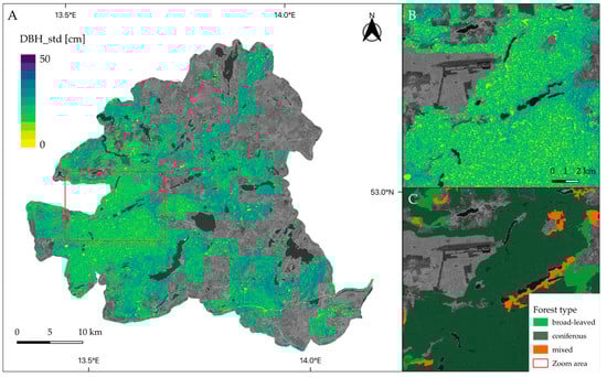
Figure 11.
Map of predicted standard deviation of tree diameter (DBH_std) for Schorfheide-Chorin (A). A closer look on the predictions is given in (B) whereas (C) provides a comparison with forest types. Predictions were masked according to the forested areas of CLC 2018 dataset. A VH-scene from Sentinel-1 is shown in the background.
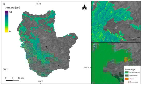
Figure 12.
Map of predicted standard deviation of tree diameter (DBH_std) for Hainich-Dün (A). A closer look on the predictions is given in (B) whereas (C) provides a comparison with forest types. Predictions were masked according to the forested areas of CLC 2018 dataset. A VH-scene from Sentinel-1 is shown in the background.
In Figure 11, extensive areas of homogeneous tree diameter distribution are visible in the western part of the Schorfheide reserve. A closer look reveals that the spatial distribution of forest cover types coincides with structural diversity patterns. For example, coniferous areas show a low standard deviation of tree diameter, whereas broad-leaved forests exhibit relatively low structural diversity. Figure 12 shows the National park Hainich and its surroundings. In the center, large, connected areas of broad-leaved, mainly beech, forests are visible that show higher variation in tree diameter.
4. Discussion
Our study showed the capability and challenges of predicting several forest key parameters with DNNs. The leave-one-out analysis of the predictors (Figure 6 and Figure 8) and the accuracy analysis with different sets of predictors (Table 4 and Table 6) gave insights on the importance of each group of predictors. Variability of species diversity was best explained by the combination of Sentinel-1 and -2 features, with the texture variables from Sentinel-2 EVI data showing the highest importance. Models based on features from Sentinel-1 alone showed the highest RMSE and poorly explained variability. Our models of DBH standard deviation, and to a lesser extent the stand density models, showed a homogeneous distribution of errors, indicating a good degree of applicability across the full range of values. On the other side, the models of species diversity had high errors at high and low values, which complicates their use for management and especially biodiversity conservation.
Our results suggest that structural diversity can be better captured by Sentinel-1 predictors alone, rather than by the combination of both optical and radar data, in agreement with other studies [26,51,52]. For instance, Fagua et al. [15], Bae et al. [26], and Brugisser et al. [16] showed that Sentinel-1 textural and temporal metrics could match the capacities of ALS systems to map forest structure parameters. Similarly, other studies showed comparable results for predictions of mean DBH in maritime [8] and boreal [30] sites. On the other hand, Sentinel-2 texture metrics have also been found useful. Farwell et al. [29] showed correlations between DBH standard deviation and EVI texture variables for 20 × 20 m plots across the US from Sentinel-2. The best predictors were entropy and homogeneity features (r2 = 0.38 and 0.52 respectively), corresponding to the evaluation of predictor importance in our study.
Regression and classification models can improve their performance with remote sensing data that covers the whole season. Improvements have been found in models of tree species diversity [13] and structural diversity [53]. For tree species diversity, we did not observe significant differences in model accuracy when using Sentinel-2 composites from different seasons (Table 4). However, by using Sentinel-1 backscatter data from the winter season, we gained higher accuracies compared to when using data from the growing and peak season (Table 6). This highlights the importance of capturing changes in forest structure across the season with radar imagery, in line with other studies [26,54].
The spectral variation hypothesis has been used before to predict tree species diversity, such as the spectral Shannon index or Rao’s Q diversity index [19]. However, in this study, Rao’s Q index did not significantly influence the predictions and was outperformed by other predictors, such as EVI texture. Only a few other authors have found Rao’s Q useful for predicting diversity, and more research is needed in this direction. For instance, Marzialetti et al. [55] found it useful for classifications of coastal dunes. Torresani et al. [13] revealed that the performance of Rao’s Q was scale and season dependent, and most studies are still limited to small sample sizes on homogeneous site conditions.
Our results show, on the one hand, the limitations of remote sensing to predict straightforward biodiversity variables such as Shannon’s index (Figure 7). Geller et al. [56] also reported that the extent to which species composition can be directly modeled with remote sensing is limited. On the other hand, we demonstrate the potential of remote sensing to predict other forest structural variables that can be used as proxies for biodiversity, such as structural heterogeneity (Figure 9). Variation in height and stand density is related to the structural diversity of stands, but they are also related to the heterogeneity of habitats for bird and insect species [22,37]. Thus, the better fits obtained with the structural variables with respect to Shannon’s index indicate that structural features can be more reliable for producing informative and spatially explicit models of biodiversity aspects. Moreover, Neumann et al. [57] praised higher relevance to structural diversity in the case of Central European forests where tree species diversity is relatively low. The focus on structural diversity has recently been used by a study of Ehbrecht et al. [24], revealing spatial matches of plant and structural diversity hotspots. However, there are other facets of structural diversity apart from size distribution that govern forest diversity and habitat complexity, such as vertical heterogeneity, deadwood standing, or bark diversity that would be valuable to detect from space across large areas [23,35] and should be further investigated.
Results of similar studies across the literature match our conclusions only to a certain extent. Farwell et al. [29] also obtained moderate correlations between texture metrics and structural parameters (r2 = 0.3–0.5) similar to our results (r2 = 0.51). Ma et al. [58] used Sentinel-2 over a broad set of European forests achieving low accuracies for tree structural traits (r2 = 0.19) but much higher when tree and leaf traits were combined (r2 = 0.55). Mallinis et al. [10] obtained a slightly higher coefficient of determination than us when predicting tree species diversity in northern Greece (r2 = 0.29 vs. 0.20), but without offering information on the error distribution or on the absence of spatial autocorrelation. A different approach was presented by Chaves et al. [59], where remote sensing was used to map relative species compositions (r2 = 0.4–0.6) across Amazonian forests, rather than absolute measurements of diversity or by doing hard classifications. Bae et al. [26] used generalized additive models to explain a broad range of biodiversity facets across temperate forests using Sentinel-1 metrics and LIDAR data. In their study, they show how accuracies increase considerably when a region is added as a predictor. This provides evidence on the importance of evaluating models outside the area where they were trained or using a very varied set of spatially uncorrelated data for model testing and validation. For example, Chrysafis et al. [11], Kampouri et al. [60], and Mallinis et al. [10] modeled forest parameters in small and homogeneous areas in northern Greece, where spatial autocorrelation is likely to obscure the true relationship between field and satellite data [61].
Support vector machines or random forests are also often used in biodiversity models. However, DL has recently been suggested to be a superior option for remote sensing studies, especially regarding its ability to automatically extract meaningful features from complex datasets [53,54]. Nevertheless, the degree to which a model can generalize well is still linked to the availability of representative field data when applied to diverse settings [47]. This was well covered by our study by using spatially independent observations from 14 different forest types whose structure and species composition depends mostly on management rather than on environmental factors [62,63].
The approach presented in this study not only gave valuable contributions to biodiversity monitoring with satellite remote sensing but also addressed an essential challenge forest inventories are facing in the course of rapidly changing forest ecosystems [64]. Due to high dynamics in the forest’s characteristics and introduced climate change mitigation, there is currently a strong need to develop multi-purpose decision-support tools for forest management as well as management practices that would rely not only on traditional forest inventories but also incorporate remote sensing datasets [64]. Thus, to meet the increasing demand for information on forest resources and their condition, the forest inventories have to become also multi-source [65]. However, operative forest inventories are time and resource-consuming. Using DL models based on multi-source datasets, the in situ collected forest data can be upscaled not only to a landscape scale but also could be used to reassess forest characteristics back in time. This, in turn, would allow to map forest conditions at large spatial scales and assess the response of habitat heterogeneity to guide forest management activities [66]. Visual assessments of the tree diameter variation maps (Figure 11 and Figure 12) allowed us to observe spatial patterns of structural heterogeneity that align with the distribution of coniferous and broad-leaved forests. Such spatially explicit maps could be used by forest managers as a guide for more detailed field sampling, to identify areas for interventions, or for planning forest management activities.
5. Conclusions
Forest inventories and biodiversity research can benefit from spatially explicit models of compositional and structural variables, especially in terms of increased areal and temporal coverage, coping with current climate change and land-use dynamics. The predictive capability of such models is, however, tied to the degree of variability of site conditions reflected in the calibration data, making it a common limiting factor of large-scale studies. To address this research gap, we applied a novel approach using deep neural networks to model tree species diversity and structural diversity based on satellite and in situ data from three forest regions covering 14 different forest types across Germany. We tested our models with a different set of predictors and recorded their particular importance. The best model was used to produce geospatial maps of structural diversity, which revealed distinctive patterns depending on the forest type.
We concluded that deep learning models based on multi-temporal Sentinel-1 imagery are capable of capturing spatial variations in forest structure across different forest types. Our study also showed the challenges that species diversity models face even when combining multi-spectral and SAR multi-temporal data. The developed approach could be applicable to model nation-wide forest biodiversity characteristics, as well as it could be used to support bottom-up investigations in biodiversity monitoring. The follow-up studies should further test the performance of this approach in other environmental settings, forest types, and address other biodiversity facets.
Author Contributions
Conceptualization, J.M. and O.D.; experimental design, J.M. and J.H.; analysis, J.H.; writing—original draft preparation, J.H., J.M. and O.D. All authors have read and agreed to the published version of the manuscript.
Funding
This research is part of the project Sensing Biodiversity Across Scales (SeBAS), grant code DU 632 1596/1-1, and has been funded by the German Research Foundation (DFG) under the priority 633 program 1374.
Data Availability Statement
This work is based on data elaborated by the forest structure core project of the Biodiversity Exploratories program (DFG Priority Program 1374). The datasets are publicly available in the Biodiversity Exploratories Information system (BexIS; https://www.bexis.uni-jena.de/ accessed on 29 December 2021). Access no. DBH standard deviation, basal area, stand density index: 22766 [67]; species inventories: 22907 [68]; forest management type: 17706 [69]; stand height: 19986 [70]. Python scripts are available at the following Github: https://github.com/jnksgit/Hoffmann-2022-rs accessed on 29 December 2021.
Acknowledgments
We thank managers of the three Exploratories Kirsten Reichel-Jung, Iris Steitz, Sandra Weithmann, Katrin Lorenzen, Juliane Vogt, Martin Gorke, Miriam Teuscher and all former managers for their work in maintaining the plot and project infrastructure; Victoria Grießmeier for giving support through the central office, Michael Owonibi and Andreas Ostrowski for managing the central database, and Markus Fischer, Eduard Linsenmair, Dominik Hessenmöller, Daniel Prati, Ingo Schöning, François Buscot, Ernst-Detlef Schulze, Wolfgang W. Weisser and the late Elisabeth Kalko for their role in setting up the Biodiversity Exploratories project. We thank the administration of the Hainich National Park, the UNESCO Biosphere Reserve Swabian Alb, and the UNESCO Biosphere Reserve Schorfheide-Chorin as well as all landowners for the excellent collaboration. We also thank Peter Schall for providing the field datasets of the second forest inventory in the BExis platform.
Conflicts of Interest
The authors declare no conflict of interest.
References
- FAO; UNEP. The state of the world’s forests. In Forests, Biodiversity and People; United Nations Food and Agriculture Organization: Rome, Italy, 2020. [Google Scholar]
- Bauhus, J.; Forrester, D.I.; Pretzsch, H. From Observations to Evidence about Effects of Mixed-Species Stands. In Mixed-Species Forests: Ecology and Management, 1st ed.; Pretzsch, H., Forrester, D.I., Bauhus, J., Eds.; Springer: Berlin, Germany, 2017; pp. 27–73. [Google Scholar]
- Austin, Z.; McVittie, A.; McCracken, D.; Moxey, A.; Moran, D.; White, P.C.L. Integrating quantitative and qualitative data in assessing the cost-effectiveness of biodiversity conservation programmes. Biodivers. Conserv. 2015, 24, 1359–1375. [Google Scholar] [CrossRef][Green Version]
- Pereira, H.M.; Ferrier, S.; Walters, M.; Geller, G.N.; Jongman, R.H.G.; Scholes, R.J.; Bruford, M.W.; Brummitt, N.; Butchart, S.H.M.; Cardoso, A.C.; et al. Essential Biodiversity Variables. Science 2013, 339, 277–278. [Google Scholar] [CrossRef] [PubMed]
- Skidmore, A.K.; Coops, N.C.; Neinavaz, E.; Ali, A.; Schaepman, M.E.; Paganini, M.; Kissling, W.D.; Vihervaara, P.; Darvishzadeh, R.; Feilhauer, H.; et al. Priority list of biodiversity metrics to observe from space. Nat. Ecol. Evol. 2021, 5, 896–906. [Google Scholar] [CrossRef]
- Holzwarth, S.; Thonfeld, F.; Abdullahi, S.; Asam, S.; Da Ponte Canova, E.; Gessner, U.; Huth, J.; Kraus, T.; Leutner, B.; Kuenzer, C. Earth Observation based Monitoring of Forests in Germany: A Review. Remote Sens. 2020, 12, 3570. [Google Scholar] [CrossRef]
- Skidmore, A.K.; Pettorelli, N.; Coops, N.C.; Geller, G.N.; Hansen, M.; Lucas, R.; Mücher, C.A.; O’Connor, B.; Paganini, M.; Pereira, H.M.; et al. Environmental science: Agree on biodiversity metrics to track from space. Nature 2015, 523, 403–405. [Google Scholar] [CrossRef]
- Morin, D.; Planells, M.; Guyon, D.; Villard, L.; Mermoz, S.; Bouvet, A.; Thevenon, H.; Dejoux, J.; Le Toan, T.; Dedieu, G. Estimation and Mapping of Forest Structure Parameters from Open Access Satellite Images: Development of a generic method with a Study Case on Coniferous Plantation. Remote Sens. 2019, 11, 1275. [Google Scholar] [CrossRef]
- Sun, H.; Hu, J.; Wang, J.; Zhou, J.; Lv, L.; Nie, J. RSPD: A Novel Remote Sensing Index of Plant Biodiversity Combining Spectral Variation Hypothesis and Productivity Hypothesis. Remote Sens. 2021, 13, 3007. [Google Scholar] [CrossRef]
- Mallinis, G.; Chrysafis, I.; Korakis, G.; Pana, E.; Kyriazopoulos, A.P. A Random Forest Modeling Procedure for a Multi-Sensor Assessment of Tree Species Diversity. Remote Sens. 2020, 12, 1210. [Google Scholar] [CrossRef]
- Chrysafis, I.; Korakis, G.; Kyriazopoulos, A.P.; Mallinis, G. Predicting Tree Species Diversity Using Geodiversity and Sentinel-2 Multi Seasonal Spectral Information. Sustainability 2020, 12, 9250. [Google Scholar] [CrossRef]
- Grabska, E.; Hostert, P.; Pflugmacher, D.; Ostapowicz, K. Forest Stand Species Mapping Using the Sentinel-2 Time Series. Remote Sens. 2019, 11, 1197. [Google Scholar] [CrossRef]
- Torresani, M.; Rocchini, D.; Sonnenschein, R.; Zebisch, M.; Marcantonio, M.; Ricotta, C.; Tonon, G. Estimating tree species diversity from space in an alpine conifer forest: The Rao’s Q diversity index meets the spectral variation hypothesis. Ecol. Inform. 2019, 52, 26–34. [Google Scholar] [CrossRef]
- Gyamfi-Ampadu, E.; Gebreslasie, M.; Mendoza-Ponce, A. Evaluating Multi-Sensors Spectral and Spatial Resolutions for Tree Species Diversity. Remote Sens. 2021, 13, 1033. [Google Scholar] [CrossRef]
- Fagua, J.C.; Jantz, P.; Burns, P.; Massey, R.; Buitrago, J.Y.; Saatchi, S.; Hakkenberg, C.; Goetz, S.J. Mapping tree diversity in the tropical forest region of Chocó-Colombia. Environ. Res. Lett. 2021, 16, 054024. [Google Scholar] [CrossRef]
- Bruggisser, M.; Dorigo, W.; Dostálová, A.; Hollaus, M.; Navacchi, C.; Schlaffer, S.; Pfeifer, N. Potential of Sentinel-1 C-Band Time Series to Derive Structural Parameters of Temperate Deciduous Forests. Remote Sens. 2021, 13, 798. [Google Scholar] [CrossRef]
- Madonsela, S.; Cho, M.A.; Ramoelo, A.; Mutanga, O. Investigating the Relationship between Tree Species Diversity and Landsat-8 Spectral Heterogeneity across Multiple Phenological Stages. Remote Sens. 2021, 13, 2467. [Google Scholar] [CrossRef]
- Khare, S.; Latifi, H.; Rossi, S. Forest beta-diversity analysis by remote sensing: How scale and sensors affect the Rao’s Q index. Ecol. Indic. 2019, 106, 105520. [Google Scholar] [CrossRef]
- Rocchini, D.; Luque, S.; Pettorelli, N.; Bastin, L.; Doktor, D.; Faedi, N.; Feilhauer, H.; Féret, J.; Foody, G.M.; Gavish, Y.; et al. Measuring ß-diversity by remote sensing: A challenge for biodiversity monitoring. Methods Ecol. Evol. 2018, 9, 1787–1798. [Google Scholar] [CrossRef]
- Torresani, M.; Rocchini, D.; Zebisch, M.; Sonnenschein, R.; Giustino, T. Testing the spectral variation hypothesis by using the RAO-Q index to estimate forest biodiversity: Effect of spatial resolution. In Proceedings of the 2018 IEEE International Geoscience and Remote Sensing Symposium, Valencia, Spain, 22–27 July 2019. [Google Scholar]
- Thom, D.; Taylor, A.R.; Seidl, R.; Thuiller, W.; Wang, J.; Robideau, M.; Keeton, W.S. Forest structure, not climate, is the primary driver of functional diversity in northeastern North America. Sci. Total Environ. 2020, 762, 143070. [Google Scholar] [CrossRef]
- Del Río, M.; Pretzsch, H.; Alberdi, I.; Bielak, K.; Bravo, F.; Brunner, A.; Condés, S.; Ducey, M.J.; Fonseca, T.; von Lüpke, N.; et al. Characterization of the structure, dynamics and productivity of mixed-species stands: A review and perspectives. Eur. J. For. Res. 2016, 135, 23–49. [Google Scholar] [CrossRef]
- Storch, F.; Dormann, C.F.; Bauhus, J. Quantifying forest structural diversity based on large-scale inventory data: A new approach to support biodiversity monitoring. For. Ecosyst. 2018, 5, 34. [Google Scholar] [CrossRef]
- Ehbrecht, M.; Seidel, D.; Annighöfer, P.; Kreft, H.; Köhler, M.; Zemp, D.C.; Puettmann, K.; Nilus, R.; Babweteera, F.; Willim, K.; et al. Global patterns and climatic controls of forest structural complexity. Nat. Commun. 2021, 12, 519. [Google Scholar] [CrossRef] [PubMed]
- Castaño-Villa, G.J.; Estevez, J.V.; Guevara, G.; Bohado-Murilla, M.; Fontúrbel, F. Differential effects of forestry plantations on bird diversity: A global assessment. For. Ecol. Manag. 2019, 440, 202–207. [Google Scholar] [CrossRef]
- Bae, S.; Levick, S.R.; Heidrich, L.; Magdon, P.; Leutner, B.J.; Wöllauer, S.; Serebryanyk, A.; Nauss, T.; Krzystek, P.; Gossner, M.M.; et al. Radar vision in the mapping of forest biodiversity from space. Nat. Commun. 2019, 10, 4757. [Google Scholar] [CrossRef] [PubMed]
- Mura, M.; McRoberts, R.E.; Chirici, G.; Marchetti, M. Estimating and mapping forest structural diversity using airborne laser scanning data. Remote Sens. Environ. 2015, 170, 133–142. [Google Scholar] [CrossRef]
- Tello, A.; Cazcarra-Bes, V.; Pardini, M.; Papathanassiou, K. Forest Structure Characterization From SAR Tomography at L-Band. IEE J. Sel. Top. Appl. Earth Obs. Remote Sens. 2018, 11, 3402–3414. [Google Scholar] [CrossRef]
- Farwell, L.S.; Gudex-Cross, D.; Anise, I.A.; Bosch, M.J.; Olah, A.M.; Radeloff, V.C.; Razenkova, E.; Rogova, N.; Silveira, E.M.O.; Smith, M.M.; et al. Satellite image texture captures vegetation heterogeneity and explains patterns of bird richness. Remote Sens. Environ. 2021, 253, 112175. [Google Scholar] [CrossRef]
- Wallner, A.; Elatawneh, A.; Schneider, T.; Knoke, T. Estimation of forest structural information using RapidEye satellite data. Forestry 2015, 88, 96–107. [Google Scholar] [CrossRef]
- Meng, J.; Li, S.; Wang, W.; Liu, Q.; Xie, S.; Ma, W. Estimation of Forest Structural Diversity Using the Spectral and Textural Information Derived from SPOT-5 Satellite Images. Remote Sens. 2016, 8, 125. [Google Scholar] [CrossRef]
- Li, Y.; Li, M.; Li, C.; Liu, Z. Forest aboveground biomass estimation using Landsat 8 and Sentinel-1A data with machine learning algorithms. Sci. Rep. 2020, 10, 9952. [Google Scholar] [CrossRef] [PubMed]
- Astola, H.; Häme, T.; Sirro, L.; Molinier, M.; Kilpi, J. Comparison of Sentinel-2 and Landsat 8 imagery for forest variable prediction in boreal region. Remote Sens. Environ. 2019, 223, 257–273. [Google Scholar] [CrossRef]
- Fischer, M.; Bossdorf, O.; Gockel, S.; Hänsel, F.; Hemp, A.; Hessenmöller, D.; Korte, G.; Nieschulze, J.; Pfeiffer, S.; Prati, D.; et al. Implementing large-scale and long-term functional biodiversity research: The Biodiversity Exploratories. Basic Appl. Ecol. 2013, 11, 473–485. [Google Scholar] [CrossRef]
- Hessenmöller, D.; Nieschulze, J.; von Lüpke, N.; Schulze, E. Identification of forest management types from ground-based and remotely sensed variables and the effects of forest management on forest structure and composition. Forstarchiv 2011, 13, 171–183. [Google Scholar]
- Schall, P.; Schulze, E.-D.; Fischer, M.; Ayasse, M.; Ammer, C. Relations between forest management, stand structure and productivity across different types of Central European forests. Basic Appl. Ecol. 2018, 32, 39–52. [Google Scholar] [CrossRef]
- Rocchini, D.; Boyd, D.S.; Féret, J.-B.; Foody, G.M.; He, K.S.; Lausch, A.; Nagendra, H.; Wegmann, M.; Pettorelli, N. Satellite remote sensing to monitor species diversity: Potentials and pitfalls. Remote Sens. Ecol. Conserv. 2016, 2, 25–36. [Google Scholar] [CrossRef]
- Pretzsch, H.; Schütze, G. Effect of tree species mixing on the size structure, density, and yield of forest stands. Eur. J. For. Res. 2015, 135, 1–22. [Google Scholar] [CrossRef]
- GEE. Sentinel-1 Algorithms in Google Earth Engine. Available online: https://developers.google.com/earth-engine/guides/sentinel1 (accessed on 29 December 2021).
- EO Research. Cloud Masks at Your Service. State-of-the-Art Cloud Masks now Available on Sentinel Hub. Available online: https://medium.com/sentinel-hub/cloud-masks-at-your-service-6e5b2cb2ce8a (accessed on 29 December 2021).
- Haralick, R.M.; Shanmugam, K.; Dinstein, I. Textural Features for Image Classification. IEEE Trans. Syst. Man Cybern. 1973, 3, 610–621. [Google Scholar] [CrossRef]
- Hofmann, S.; Everaars, J.; Schweiger, O.; Frenzel, M.; Bannehr, L. Modeling patterns of pollinator species richness and diversity using satellite image texture. PLoS ONE 2017, 12, e0185591. [Google Scholar] [CrossRef]
- Tuanmu, M.-N.; Jetz, W. A global, remote sensing-based characterization of terrestrial habitat heterogeneity for biodiversity and ecosystem modeling. Glob. Ecol. Biogeogr. 2015, 24, 1329–1339. [Google Scholar] [CrossRef]
- Rocchini, D.; Marcantonio, M.; Ricotta, C. Measuring Rao’s Q diversity index from remote sensing: An open source solution. Ecol. Indic. 2017, 72, 234–238. [Google Scholar] [CrossRef]
- Khare, S.; Latifi, H.; Rossi, S. A 15-year spatio temporal analysis of plant ß-diversity using Landsat time series derived Rao’s Q index. Ecol. Indic. 2021, 121, 107105. [Google Scholar] [CrossRef]
- Géron, A. Hands-on Machine Learning with Scikit-Learn, Keras and TensorFlow: Concepts, Tools, and Techniques to Build Intelligent Systems, 2nd ed.; O’Reilly Media, Inc.: Beijing, China, 2016. [Google Scholar]
- Kattenborn, T.; Leitloff, J.; Schiefer, F.; Hinz, S. Review on Convolutional Neural Networks (CNN) in vegetation remote sensing. ISPRS J. Photogramm. Remote Sens. 2021, 173, 24–49. [Google Scholar] [CrossRef]
- Hoeser, T.; Kuenzer, C. Object Detection and Image Segmentation with Deep Learning on Earth Observation Data: A Review-Part I: Evolution and Recent Trends. Remote Sens. 2020, 12, 1667. [Google Scholar] [CrossRef]
- Zhu, X.X.; Tuia, D.; Mou, L.; Xia, G.; Zhang, L.; Xu, F.; Fraundorfer, F. Deep Learning in Remote Sensing: A Comprehensive Review and List of Resources. IEEE Geosci. Remote Sens. Mag. 2017, 5, 8–36. [Google Scholar] [CrossRef]
- McElhinny, C.; Gibbons, P.; Brack, C.; Bauhus, J. Forest and woodland stand structural complexity: Its definition and measurement. For. Ecol. Manag. 2005, 218, 1–24. [Google Scholar] [CrossRef]
- Bellis, L.M.; Pidgeon, A.M.; Radeloff, V.C.; St-Louis, V.; Navarro, J.L.; Martella, M.B. Modeling habitat suitability for greater rheas based on satellite image texture. Ecol. Appl. 2008, 18, 1956–1966. [Google Scholar] [CrossRef]
- Joshi, N.; Mitchard, E.T.A.; Brolly, M.; Schumacher, J.; Fernández-Landa, A.; Johannsen, V.K.; Marchamalo, M.; Fensholt, R. Understanding ‘saturation’ of radar signals over forests. Sci. Rep. 2017, 7, 3505. [Google Scholar] [CrossRef]
- Chang, T.; Rasmussen, B.P.; Dickson, B.G.; Zachmann, L.J. Chimera: A Multi-Task Recurrent Convolutional Neural Network for Forest Classification and Structural Estimation. Remote Sens. 2019, 11, 768. [Google Scholar] [CrossRef]
- Astola, H.; Seitsonen, L.; Halme, E.; Molinier, M.; Lönnqvist, A. Deep Neural Networks with Transfer Learning for Forest Variable Estimation Using Sentinel-2 Imagery in Boreal Forest. Remote Sens. 2021, 13, 2392. [Google Scholar] [CrossRef]
- Marzialetti, F.; Di Febbraro, M.; Malavasi, M.; Giulio, S.; Rosario Acosta, A.T.; Carranza, L.M. Mapping Coastal Dune Landscape through Spectral Rao’s Q Temporal Diversity. Remote Sens. 2020, 12, 2315. [Google Scholar] [CrossRef]
- Geller, G.N.; Halpin, P.N.; Helmuth, B.; Hestir, E.L.; Skidmore, A.; Abrams, M.J.; Aguirre, N.; Blair, M.; Botha, E.; Colloff, M.; et al. Remote Sensing of Biodiversity. In The GEO Handbook on Biodiversity Observation Networks, 1st ed.; Walters, M., Scholes, R.J., Eds.; Springer: Berlin, Germany, 2017; pp. 187–210. [Google Scholar]
- Neumann, M.; Starlinger, F. The significance of different indices of stand structure and diversity in forests. For. Ecol. Manag. 2001, 145, 91–106. [Google Scholar] [CrossRef]
- Ma, X.; Mahecha, M.D.; Migliavacca, M.; van der Plas, F.; Benavides, R.; Ratcliffe, S.; Kattge, J.; Richter, R.; Musavi, T.; Baeten, L.; et al. Inferring plant functional diversity from space: The potential of Sentinel-2. Remote Sens. Environ. 2019, 233, 111368. [Google Scholar] [CrossRef]
- Chaves, P.P.; Zuquim, G.; Ruokolainen, K.; Van Doninck, J.; Kalliola, R.; Gómez Rivero, E.; Tuomisto, H. Mapping Floristic Patterns of Trees in Peruvian Amazonia Using Remote Sensing and Machine Learning. Remote Sens. 2020, 12, 1523. [Google Scholar] [CrossRef]
- Kampouri, M.; Kolokoussis, P.; Argialas, D.; Karathanassi, V. Mapping of forest tree distribution and estimation of forest biodiversity using Sentinel-2 imagery in the University Research Forest Taxiarchis in Chalkidiki, Greece. Geocarto Int. 2019, 34, 1273–1285. [Google Scholar] [CrossRef]
- Ploton, P.; Mortier, F.; Réjou-Méchain, F.; Barbier, M.; Picard, N.; Rossi, V.; Dormann, C.; Cornu, G.; Viennois, G.; Bayol, N.; et al. Spatial validation reveals poor predictive performance of large-scale ecological mapping models. Nat. Commun. 2020, 11, 4540. [Google Scholar] [CrossRef]
- Neff, F.; Brändle, M.; Ambarli, D.; Ammer, C.; Bauhus, J.; Boch, S.; Hölzel, N.; Klaus, V.H.; Kleinebecker, T.; Gossner, M.M. Changes in plant-herbivore network structure and robustness along land-use intensity gradients in grasslands and forests. Sci. Adv. 2021, 7, eabf3985. [Google Scholar] [CrossRef]
- Felipe-Lucia, M.R.; Soliveres, S.; Penone, C.; Fischer, M.; Ammer, C.; Bolch, S.; Boeddinghaus, R.S.; Bonkrowski, M.; Buscot, F.; Fiore-Donno, A.M.; et al. Land-use intensity alters networks between biodiversity, ecosystem functions and services. Proc. Natl. Acad. Sci. USA 2020, 117, 28140–28149. [Google Scholar] [CrossRef]
- Tomppo, E.; Olsson, H.; Ståhl, G.; Nilsson, M.; Hagner, O.; Katila, M. Combining national forest inventory field plots and remote sensing data for forest databases. Remote Sens. Environ. 2008, 112, 1982–1999. [Google Scholar] [CrossRef]
- Wallner, A.; Friedrich, S.; Geier, E.; Meder-Hokamp, C.; Wei, Z.; Kindu, M.; Tian, J.; Döllerer, M.; Schneider, T.; Knoke, T. A remote sensing-guided forest inventory concept using multispectral 3D and height information from ZiYuan-3 satellite data. Forestry 2021, 88, 1–16. [Google Scholar] [CrossRef]
- Thonfeld, F.; Gessner, U.; Holzwarth, S.; Kriese, J.; da Ponte, E.; Huth, J.; Kuenzer, C. A First Assessment of Canopy Cover Loss in Germany’s Forests after the 2018–2020 Drought Years. Remote Sens. 2022, 14, 562. [Google Scholar] [CrossRef]
- Schall, P.; Ammer, C. Stand Structural Attributes Based on 2nd Forest Inventory, All Forest EPs, 2014–2018. Biodiversity Exploratories Information System (BexIS). Dataset ID = 22766. Available online: https://www.bexis.uni-jena.de/ (accessed on 29 December 2021).
- Schall, P.; Ammer, C. Stand Composition Based on 2nd Forest Inventory, All Forest EPs, 2014–2018. Biodiversity Exploratories Information System (BexIS). Dataset ID = 22907. Available online: https://www.bexis.uni-jena.de/ (accessed on 29 December 2021).
- Schall, P.; Ammer, C. New Forest Type Classification of All Forest EPs, 2008–2014. Biodiversity Exploratories Information System (BexIS). Dataset ID = 17706. Available online: https://www.bexis.uni-jena.de/ (accessed on 29 December 2021).
- Ehbrecht, M.; Ammer, C.; Schall, P. Effective Number of Layers from LiDAR, Forest, EP, 2014. Biodiversity Exploratories Information System (BexIS). Dataset ID = 19986. Available online: https://www.bexis.uni-jena.de/ (accessed on 29 December 2021).


Publisher’s Note: MDPI stays neutral with regard to jurisdictional claims in published maps and institutional affiliations. |
© 2022 by the authors. Licensee MDPI, Basel, Switzerland. This article is an open access article distributed under the terms and conditions of the Creative Commons Attribution (CC BY) license (https://creativecommons.org/licenses/by/4.0/).