Article

Filling Temporal Gaps within and between GRACE and GRACE-FO Terrestrial Water Storage Records: An Innovative Approach

1
Center for Water Supplies Studies, Department of Physical and Environmental Sciences, Texas A&M University-Corpus Christi, 6300 Ocean Drive, Corpus Christi, TX 78412, USA
2
Jet Propulsion Laboratory, California Institute of Technology, Pasadena, CA 91109, USA
*
Author to whom correspondence should be addressed.
Remote Sens. 2022, 14(7), 1565; https://doi.org/10.3390/rs14071565
Submission received: 17 February 2022 / Revised: 16 March 2022 / Accepted: 21 March 2022 / Published: 24 March 2022

Abstract

:
Temporal gaps within the Gravity Recovery and Climate Experiment (GRACE) (gap: 20 months), between GRACE and GRACE Follow-On (GRACE-FO) missions (gap: 11 months), and within GRACE-FO record (gap: 2 months) make it difficult to analyze and interpret spatiotemporal variability in GRACE- and GRACE-FO-derived terrestrial water storage (TWSGRACE) time series. In this study, an overview of data and approaches used to fill these gaps and reconstruct the TWSGRACE record at the global scale is provided. In addition, the study provides an innovative approach that integrates three machine learning techniques (deep-learning neural networks [DNN], generalized linear model [GLM], and gradient boosting machine [GBM]) and eight climatic and hydrological input variables to fill these gaps and reconstruct the TWSGRACE data record at both global grid and basin scales. For each basin and grid cell, the model performance was assessed using Nash–Sutcliffe efficiency coefficient (NSE), correlation coefficient (CC), and normalized root-mean-square error (NRMSE), a leader model was selected based on the model performance, and variables that significantly control leader model outputs were defined. Results indicate that (1) the leader model reconstructed the TWSGRACE with high accuracy over both grid and local scales, particularly in wet and low anthropogenically active regions (grid scale: NSE = 0.65 ± 0.20, CC = 0.81 ± 0.13, and NSE = 0.56 ± 0.16; basin scale: NSE = 0.78 ± 0.14, CC = 0.89 ± 0.07, and NRMSE = 0.43 ± 0.14); (2) no single model was flawless in reconstructing the TWSGRACE over all grids or basins, so a combination of models is necessary; (3) basin-scale models outperform grid-scale models; (4) the DNN model outperforms both GLM and GBM at the basin scale, whereas the GBM outperforms at the grid scale; (5) among other inputs, the Global Land Data Assimilation System (GLDAS)-derived TWS controls the model performance on both basin and grid scales; and (6) the reconstructed TWSGRACE data captured extreme climatic events over the investigated basins and grid cells. The developed approach is robust, effective, and could be used to accurately reconstruct TWSGRACE for any hydrologic system across the globe.

1. Introduction

The Gravity Recovery and Climate Experiment (GRACE) mission launched jointly by the U.S. National Aeronautics and Space Administration and the German Aerospace Center on 17 March 2002 was designed to map both spatial variability in the Earth’s static gravity field and the spatiotemporal variations in Earth’s gravity field with unprecedented accuracy [1]. The spatiotemporal variability in gravity field solutions delivered by the GRACE mission is directly related to the natural and anthropogenic variations in terrestrial water storage (TWS) components such as surface water, groundwater, soil moisture, permafrost, snow, ice, and wet biomass [2]. The GRACE-derived TWS (TWSGRACE) empowers the scientific community to address previously unresolvable questions in hydrology, oceanology, cryosphere, and solid Earth fields at both regional and global scales [3,4,5,6,7,8,9,10,11,12,13,14,15,16,17,18,19,20,21]. However, the global monthly TWSGRACE record (April 2002–June 2017) suffers from temporal gaps (20 months) caused by battery performance issues with approximately 10% of the TWSGRACE record missing.
Because of the impressive success of the GRACE mission, the GRACE Follow-On (GRACE-FO) mission launched in May 2018 and is continuing the extremely successful work of its predecessor [22]. However, there is an 11-month gap in TWS data (July 2017–May 2018) between the two missions. Two additional months are missing from the current GRACE-FO record (August 2018–September 2018). Currently, an estimated 15% of the available TWSGRACE data record is missing from the combined GRACE and GRACE-FO missions (April 2002–April 2021). In this study, the term TWSGRACE refers to both the GRACE- and GRACE-FO-derived TWS records (i.e., the combined data record).
Similar to any other temporal dataset, temporal gaps in TWSGRACE hinder their analysis and interpretation [23,24,25]. Gaps in TWSGRACE introduce errors in amplitude and phase of the annual cycle, residual variabilities, and secular trends, and increase the level of uncertainty in their spectral modeling [26]. Long gaps could also obscure the temporal patterns of TWS data and consequently distort the results of any statistical analysis [27].
In this article, we provide an overview of previous approaches that have been used to reconstruct, and/or fill gaps in the TWSGRACE record and discuss the advantages and limitations of each approach. In addition, we provide an innovative approach to fill current gaps in the TWSGRACE record, between GRACE and GRACE-FO missions, and within the GRACE-FO record. Specifically, three machine learning techniques (generalized linear model [GLM], gradient boosting machine [GBM], and deep-learning neural networks [DNN]) and eight climatic and hydrological input variables were integrated and used to reconstruct TWSGRACE data at both the grid (1° × 1°; total grid points: 14,310) and basin (62 global watersheds; Figure 1) scales. For each basin and grid cell, the model performance was assessed for GLM, GBM, and DNN models, and a “leader model” was selected. In this article, the leader model is defined as the model that combines the best (highest statistical performance during the testing phase) of the three models. Model inputs that significantly control TWSGRACE variability in each basin and grid were also identified.

2. Filling Temporal Gaps in TWSGRACE Record: An Overview

Several studies have been conducted to reconstruct the TWSGRACE using different datasets and approaches at both grid and basin scales (Table 1). Datasets that have been used to reconstruct the TWSGRACE include measured and modeled hydroclimatic and/or gravimetric datasets. The hydroclimate variables were used to reconstruct TWSGRACE by correlating the spatiotemporal variability in these variables with the spatiotemporal variability in TWSGRACE. Examples of the climatic variables include, but are not limited to, temperature, rainfall, sea surface temperature, and climate indices [25,28,29,30,31,32,33,34,35,36,37]. Hydrological variables include soil moisture, runoff, water level, and evapotranspiration [25,33,34,36,38,39,40,41,42].
Gravimetric datasets from various low Earth orbiting (LEO) satellite missions were used to reconstruct, and fill gaps within, the TWSGRACE. For instance, the Geodetic satellite laser ranging (SLR) data that provide temporal variations of the Earth’s gravity field at the lowest degrees of the spherical harmonic spectrum were used to fill the gap in TWSGRACE [37,43,44,45,46]. Low-resolution gravity models derived from the European Space Agency (ESA)’s Swarm satellite were used to recover the temporal variations in Earth’s gravity field [47] and reconstruct the TWSGRACE [48,49,50]. These products, however, have very coarse resolution (~1500 km) compared to TWSGRACE data [42], which limits their application in reconstruction TWSGRACE data.
Several techniques used TWSGRACE data along with different hydroclimatic and hydrologic variables to fill TWSGRACE data gaps. These include interpolation, signal decomposition, use of land surface models (LSMs) outputs, water balance, data assimilation, and statistical and data mining techniques (Table 1).
Interpolation of the neighboring months has been widely used to fill TWSGRACE data gaps [7,8,27]. Linear interpolation techniques, however, are less accurate in mapping nonlinear systems such as TWSGRACE [51], especially where two or more successive monthly values are missing (e.g., 11-month gap between the GRACE and GRACE-FO missions). In addition, other interpolation techniques (e.g., spline) are less accurate at mapping extreme values such as those associated with droughts and floods, and they usually suffer from smoothing effects [52].
The Singular Spectrum Analysis (SSA) techniques have been used to fill the missing TWSGRACE data [50,53,54,55] given that SSA is able to extract significant information from short and noisy time series by decomposing it into a trend, annual/seasonal signal, and noise without any prior physical and dynamical knowledge that affects time series [56]. However, SSA is reported to have distorted reconstruction results [50].
LSM-derived TWS outputs have also been used as proxies for TWSGRACE data. This approach, however, depends on the degree to which these models can simulate natural episodic events (e.g., droughts or floods), which in turn are dependent on the physics and structure of these LSMs, and on the resolution, coverage, and accuracy of the meteorological forcing datasets [57]. A recent study over Africa [3] indicated that some of the LSMs result in overestimation of winter TWS values and underestimates of summer values when compared to TWSGRACE. Globally, LSMs underestimate TWSGRACE trends [58] and are unable to capture seasonal TWSGRACE amplitudes [59]. Although such models can potentially simulate TWSGRACE variabilities caused by natural phenomena, they are also less successful at simulating variabilities caused by anthropogenic influences because these forcings are typically not captured in the LSMs inputs [60,61,62,63].
Table 1. Review of previous TWSGRACE reconstruction data and techniques.
ReferenceScale/RegionApproach †Inputs *
Becker et al. [38]Grid (Amazon)CorrelationGRACE, Water level
Pan et al. [36]Basin (global)Data assimilation GRACE, LSM, P, ET
De Linage et al. [35]Basin (Amazon)MLRPacific and Atlantic SST
Long et al. [33]Basin (Southwest China)ANNSMS, P, T
Forootan et al. [29]Basin/Grid (West Africa)ICA, ARXSST, P
Sośnica et al. [46]Grid (global)LRSLR, GRACE
Zhang et al. [64]Basin (Yangtze)ANNSMS
Nie et al. [65]Basin (Amazon)LRGRACE, GLDAS
Talpe et al. [43]Grid (Greenland and Antarctica)PCASLR, GRACE
Humphrey et al. [30]Grid (global)MLRP, T
Yang et al. [41]Basin (NW China)ANN, GLM, RF, SVMGRACE, GLDAS
Chen et al. [28]Basin (Northeast China)GRNNP, T
Ahmed et al. [25]Basin (Africa)NARXP, ET, NDVI, T
Hasan et al. [39]Basin (Africa)ARXGLDAS, ENSO
Yin et al. [34]Basin (China)MLR P, ET, runoff
Meyer et al. [49]Grid (Arctic and Antarctic)LRSLR, Swarm,GRACE
Humphrey and Gudmundsson [66] Grid (global)MLRGRACE, P
Ferreira et al. [67]Grid (West Africa)NARXP, ET, T, SMS, climate indices
Sun et al. [68]Grid (India)CNNGRACE, GLDAS
Li et al. [53]Basin (China)SSA, ARIMAGRACE, GLDAS
Jing et al. [69]Basin (Nile)RF, XGBGRACE, GLDAS
Kenea et al. [31]Basin (Ethiopia)ESMSST, P
Jing et al. [40]Basin (China)RF, LRGRACE, GLDAS
Zhu et al. [70]Grid (global)SSAGRACE
Li et al. [32]Grid/Basin (global)MLR, ANN, ARXP, T, SST, climate indices
Forootan et al. [48]Grid/Basin (global)ICAGRACE, Swarm
Sun et al. [71]Grid/Basin (global)DNN, MLR, SARIMAXGRACE, GLDAS, P, T
Sohoulande et al. [72]Grid (United States)MVSP, T, potential ET
Jing et al. [73]Basin (regional)RF, XGBCRU,GLDAS
Sun et al. [42]Grid/Basin (United States)AutoMLGLDAS, climate indices, P, T
Li et al. [37]Grid (global)ANN, ARX, MLRP, SST, T, climate indices
Jeon et al. [74]Grid/Basin (global)CNNT, ET, P
Yu et al. [75]Grid (Canada)CNNGRACE,EALCO-TWS
Tang et al. [76]Basin (Lancang-Mekong)RFGLDAS,CRU
Yang et al. [77]Grid (Australia)LSRGRACE, modeled TWS
Wang et al. [55]Basin (Global)SSAGRACE, Swarm
Löcher and Kusche [45]Grid (global)EOFSLR
Yi and Sneeuw [52]Grid/Basin (global)SSASwarm, GRACE
Gyawali et al. [20]Basin (Texas coast)ANN, MLRP, T, NLDAS-TWS
Mo et al. [78]Grid/Basin (Global)BCNNP, T, ERA5L-TWSA, CWSC
† ANN: artificial neural network; DNN: deep neural network; CNN: convolutional neural network; BCNN: Bayesian convolutional neural networks; GLM: generalized linear model; SVM: support vector machines; RF: random forest; MLR: multilinear regression; XGB: extreme gradient boosting; AutoML: automated machine learning; ARX: autoregressive exogenous; NARX: nonlinear autoregressive with exogenous; SARIMA: seasonal auto-regressive integrated moving average with exogenous variables; GRNN: general regression neural network; SSA: singular spectrum analysis; ICA: Independent component analysis; ESM: empirical statistical model; LR: linear regression; MVS: multivariate statistics; LSR: least square regression; EOF: empirical orthogonal function; * P: precipitation; T: temperature; SST: sea surface temperature; ET: evapotranspiration; SMS: soil moisture; NDVI: normalized difference vegetation index; NLDAS: North American land data assimilation system; ENSO: El Niño and the Southern Oscillation; EALCO: Ecological Assimilation of Land and Climate Observation; CRU: Climatic Research Unit; ERA5L-TWSA: ERA5-land Derived TWSA; and CWSC: cumulative water storage change.
Basin-scale water balance calculations that combine rainfall, evapotranspiration, and runoff have also been used to reconstruct TWSGRACE [79]. For example, Pan et al. [36] used this approach to reconstruct the TWSGRACE over 32 global river basins using ground-based and remote sensing observations and LSM simulations from 1984 to 2006. Biases in rainfall and/or evapotranspiration estimates, in addition to the lack of runoff data availability, hinder the effectiveness of this approach. In addition, this technique does not take advantage of the full scope of information provided by the current TWSGRACE record (e.g., anthropogenic and natural variabilities).
In recent years, data assimilation techniques have been increasingly used to reconstruct the TWSGRACE, with higher spatial and temporal resolution. Assimilation techniques integrate TWSGRACE with LSMs to enhance the model performance. For example, Eicker et al. [80] used an ensemble-based Kalman filter approach to assimilate TWSGRACE into the Water Global Analysis and Prognosis (WaterGAP) LSM to predict TWS on both basin and grid scales over the United States. Assimilation of TWSGRACE data into several LSMs was performed to improve the models’ output, particularly the output of the TWS component [81,82,83,84,85,86,87]. The assimilation technique is useful to horizontally downscale coarse resolution and vertically disaggregate TWSGRACE data. However, because there is a mismatch in spatial and temporal resolution between TWSGRACE and LSMs, and the error properties of the TWSGRACE data are complex, the assimilation process requires complex algorithms that can be computationally extensive [88].
The statistical and data mining techniques correlate variabilities in TWSGRACE with changes in different hydroclimatic and hydrologic variables such as precipitation, temperature, vegetation indices (e.g., normalized difference vegetation index [NDVI]), evapotranspiration, soil moisture, and Global Land Data Assimilation System (GLDAS)-derived TWS (TWSGLDAS). These approaches offer an advantage over other methods because they facilitate the reconstruction of TWSGRACE at basin or grid scales. The former approach averages relevant variables over a specific basin [31,35,38,89], whereas the latter generates these variables for each pixel (e.g., 1° × 1°) [30,48,66,70]. Examples of these techniques used include artificial neural network (ANN) [20,32,33,41,42,64], convolutional neural network (CNN) [68,74,75,78], deep neural network (DNN) [71], generalized linear model (GLM) [41], random forest (RF) [40,76,90], support vector machines (SVM) [41,90], multilinear regression (MLR) [20,25,34,68], extreme gradient boosting (XGB) [69,73,90], automated machine learning (AutoML) [42], autoregressive exogenous (ARX) and nonlinear autoregressive with exogenous (NARX) [32,37,39], linear statistical models [29,30,35,66,72,77], seasonal auto-regressive integrated moving average (ARIMA) with exogenous variables (SARIMA) [71], and general regression neural network (GRNN) [28].
Note each of these techniques has its own shortcomings. For example, they (1) were reported to be effective only for large-scale (area >200,000 km2) basins [91], (2) require knowledge of basin characteristics (e.g., percent forest cover, irrigated areas) that might not be available for all basins [91], (3) are restricted to specific areas such as those experiencing strong ocean–land–atmosphere interactions [29,92], (4) perform better when linear relationships were reported between model inputs and TWSGRACE [20], and, (5) are less effective in reconstructing TWSGRACE trends in hydrogeologic systems affected by anthropogenic activities [71]. Moreover, all of these approaches either (1) compare the performance of multiple models without pinpointing to the leader model for each basin or grid cell on a global scale, (2) select the leader model without providing a comprehensive comparison of different models’ performance at each grid or basin on a global scale, or (3) pinpoint the leader model without discussing the model inputs that significantly control TWSGRACE variability at each grid or basin. In addition, none of these models were used to fill the gap between GRACE and GRACE-FO missions globally on both basin and grid scales. This study offers innovative solutions to overcome the majority of these limitations. Globally, for both grid and basin scales, a leader model was defined as the model that combines the best (highest statistical performance during the testing phase) of the three models (GLM, GBM, and DNN). The relative importance of the leader model inputs was also provided.

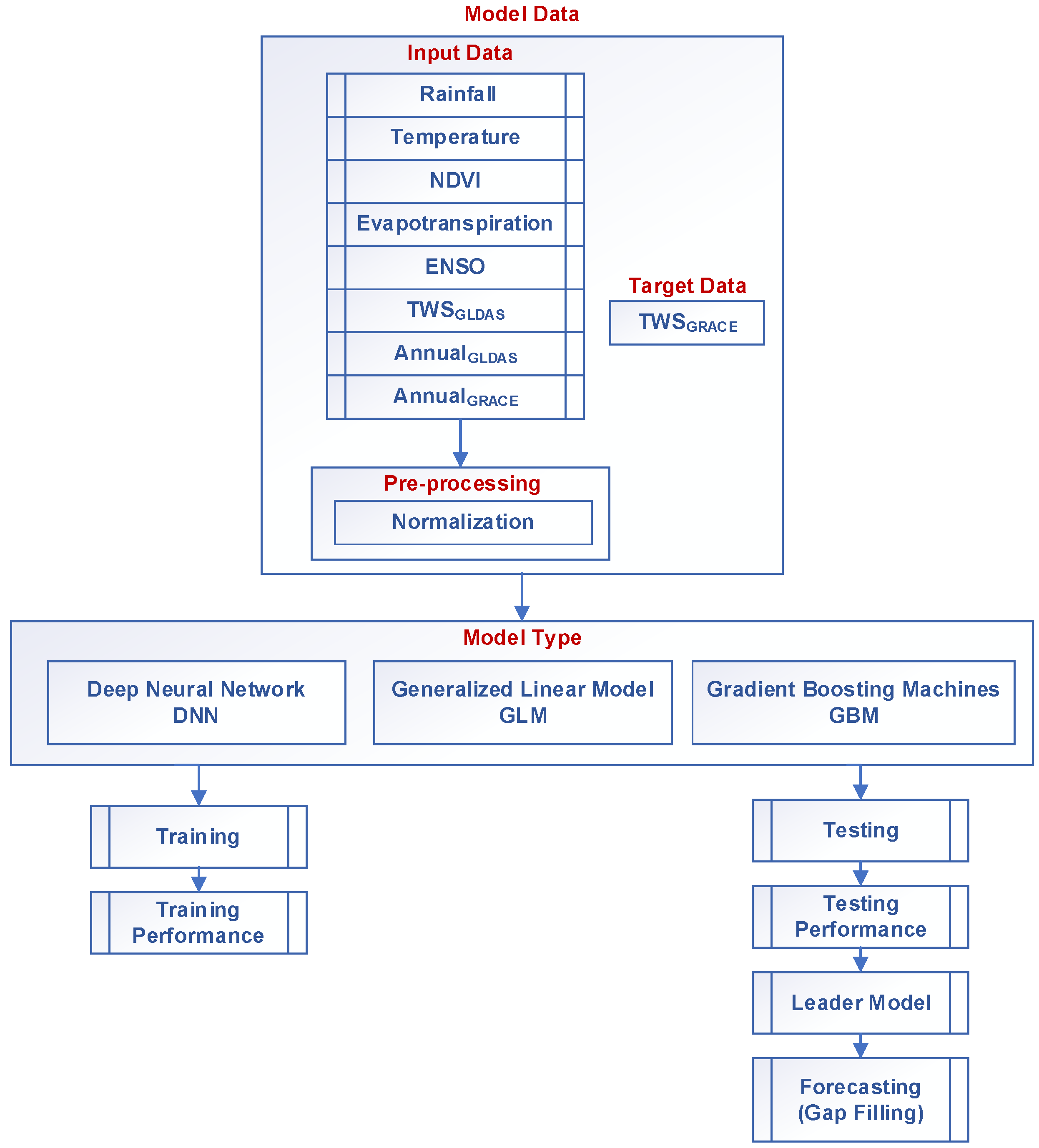
3. Innovative Approach to Fill Gaps in TWSGRACE Record

In this study, three different machine learning algorithms GLM, GBM, and DNN are used to fill the TWSGRACE gaps globally, on both basin and grid (total grid points: 14,310) scales. Different types of algorithms were selected to better improve the fitting results of the TWSGRACE data. Sixty-two major global river basins covering a wide range of climatic, hydrologic, and geologic settings were included in this study (Figure 1). Table A1 (Appendix A) lists the name, area, and climate setting of each of these basins. A comprehensive set of hydrological and climatic variables including rainfall, temperature, evapotranspiration, TWSGLDAS, NDVI, ENSO climate index, and annual cycles derived from GRACE (AnnualGRACE) and GLDAS (AnnualGLDAS) were used as model inputs. These input variables were selected to best represent spatiotemporal variations in TWSGRACE data globally [25,66,71]. The TWSGRACE data represent the model output (target).
Figure 1. Spatial distribution of the 62 global watersheds (names are shown in the bottom) examined in this study. Also shown are the simplified Köppen–Geiger global climate zones [93].
Remotesensing 14 01565 g001
The model inputs (e.g., rainfall, temperature, evapotranspiration, TWSGLDAS, NDVI, ENSO, AnnualGRACE, and AnnualGLDAS) and target (e.g., TWSGRACE) data were divided randomly into training (65%), validation (15%), and testing (20%) sets. Out of the available time series (April 2002–April 2020; 184 months), 147 months were randomly selected to train and validate the model, and 37 months were randomly selected to test the model performance. Random selection of the training and testing sets enables the designated algorithms to better understand, not memorize, the temporal variability in TWSGRACE, hence leading to better predictions of TWSGRACE gaps. The data gaps in the GRACE record (20 months), between GRACE and GRACE-FO (11 months), and in the GRACE-FO mission (2 months) were used as a forecasting (e.g., gap filling) set (total: 33 months).
The three models were compared based on their performances for the training, validation, and testing phases using various statistical parameters as presented in Section 3.3. To avoid overfitting for each model, the early stopping criteria were implemented using the mean square error (MSE) as a stopping metric, with stopping rounds of 5 and stopping tolerance of 0.0001. The selected leader model was the one that had the highest statistical performance during the testing phase of the three models (GLM, GBM, and DNN). In the following sections, a comprehensive description of each model and the details of the model input data and performance measures are presented.

3.1. Machine Learning Models

The GLM, GBM, and DNN machine learning models were used to quantify the relationship between model inputs, on the one hand, and the TWSGRACE data, on the other hand. Each of these models represent a member of a machine learning family that has been extensively used to model a complex time series such as TWSGRACE. Different model types were used to ensure the improvement of model fit with the actual TWSGRACE data.

3.1.1. Generalized Linear Model (GLM)

The GLM is a flexible and extended form of the ordinary linear regression model and is represented by the following equation:
y i = β 0 + β i x i + e i ,  
where β 0 and β i represent the intercept and the weight terms, respectively, and ei is the Gaussian random variable, which is the error/noise in the model. The linear regression model assumes that y i and error are normally distributed, and xi has constant variance. In the GLM, the errors and y i do not need to be normally distributed assuming a distribution from an exponential family, which allows variable variance and a nonlinear relationship between target and input variables [94]. The GLM uses absolute values of t-statistics to estimate the importance of a variable [95]. More details about GLMs can be found in Coxe et al. [96].

3.1.2. Gradient Boosting Machine (GBM)

The GBM model is one of the most powerful supervised machine learning approaches, and it has already shown promising performance in both regression and classification problems [97]. The GBM is a tree-based improved stepwise additive boosting algorithm that sequentially fits new tree-based models [98] and reduces bias and variance by combining an ensemble of weak learners as a weighted sum. The model optimizes key hyperparameters (e.g., number of trees, depth of trees, and learning rate) and offers an optimal technique to handle unbalanced datasets [99]. The simplified equations for GBM are expressed as follows:
F m ( x ) = F m 1 ( x ) + γ m h m ( x ) ,  
γ m = argmin γ   i = 1 n L ( y i ,   F m 1 ( x i ) + γ h m ( x i ) ) ,
where Fm(x) is the output, L ( y i ,   F ( x i ) ) is the loss function, γ m is the residual, h m ( x i ) is the base/weak learner, and x i and y i are the input and target variables, respectively. We set a varying learning rate from 0.01 to 0.1 with a 0.005 increment, sample rate from 0.1 to 1 with a 0.05 increment, maximum tree depth from 1 to 20, and number of maximum trees to 50. The model tries all possible combinations of these hyperparameters and reports the best training results. In the GBM, the variable importance is derived based on the knowledge of the variance on the input variables [100]. A more detailed description of the GBM model is presented in Friedman [98] and Friedman [97].

3.1.3. Deep Neural Network (DNN)

The DNN structure is complex compared to traditional ANNs, which allows the DNN to automatically extract deeper and more complicated relationships between model inputs and outputs [101]. The DNN is composed of interconnected organized layered neurons. The first layer of neurons is called the input node. It receives information from input data and combines and passes the data to the next layer through transformation. The last layer in the network is called the output layer and produces the output of the model. The layers between input and output are called hidden layer(s). The input–output relationship for each layer is given by this equation [102]:
y i j = ( M k = 1 j 1 w i k j 1 y i j 1 + w i 0 j 1 ) , i = 1 ,   2 ,     J k ,
where j represents the layer index, y i j 1 is the jth layer input with dimension M j−1, Jk represents the number of hidden neurons used, wik are elements of the weight matrix, wi0 represents bias term in model, is the activation function, and y i j is the model output. We set the number of hidden layers to 2 and 3 layers each with 200 neurons, activation function to rectifier, varying learning rate from 0 to 0.1 with a 0.001 increment, and input dropout ratio from 0.1 to 0.2 with a 0.05 increment. In DNN, the variable importance is derived from the weights of neurons between the input layers and hidden layers [103]. A more detailed description of the DNN model is presented by Bengio [104].

3.2. Input and Target Data

The model input data include eight variables (Figure 2) that combine remote sensing, hydrological, and climatic datasets (i.e., rainfall, temperature, evapotranspiration, TWSGLDAS, NDVI, ENSO, AnnualGRACE, and AnnualGLDAS). The model target data are represented by the TWSGRACE. Input variables were reported to have controls on TWSGRACE. For example, an increase in rainfall due to changes in ENSO will increase soil moisture (e.g., TWSGLDAS), NDVI, and consequently TWS, whereas an increase in temperature will increase evaporation and decrease TWS [105,106,107]. A lag of 3 months was used for input time series to account for the reported lags between TWSGRACE and the model inputs. The TWSGRACE exhibits couple months lag given the time it takes for any hydrological system to respond to any spatiotemporal changes in rainfall and temperature [13,42,71,108].
The input and target variables were obtained from different sources with different grid size that range from 0.01° (1 km) to 1° (~110 km). For the grid-scale predictions, the model inputs and target variable were resampled at 1° × 1° using the nearest neighbor resampling technique to make all variables comparable and also to make the TWSGRACE reconstruction results comparable to the published ones. We generated a time series for each input (total: 8) and target (total: 1) variable at each grid cell (total: 14,310). For basin scale prediction, the raw input and target variables were averaged over each of the 62 investigated basins to generate a time series for each variable at the basin scale.
The input data were normalized between 0 to 1 using the following equation:
x ¯ i =   x i x min x max x min
where x ¯ i is normalized value for   x i and xmin and xmax are minimum and maximum values for the time series.
The annual cycle for TWSGRACE and TWSGLDAS were calculated by simultaneously fitting trend and seasonal (e.g., annual and semiannual) terms to each time series according to the following equation:
S = a + b · t + c · sin ω t + d · cos ω t + e · sin 2 ω t + f · cos 2 ω t
where S is TWSGRACE or TWSGLDAS time series, a is the offset, b is the long-term trend, c and d are annual terms, e and f are semi-annual terms, t is the time vector, and ω = 2π/T with T defined as the annual period.

3.2.1. GRACE-Derived TWS (TWSGRACE)

The latest version of GRACE mass concentration (mascon) products (RL06M) provided by the Jet Propulsion Laboratory (JPL) was used in this study. The JPL-RL06M data are available at https://grace.jpl.nasa.gov (accessed on 10 December 2021) on a 0.5° × 0.5° grid scale; however, the native resolution is 3° × 3° equal-area caps [109]. The TWSGRACE product (expressed in equivalent water thickness) for the April 2002 to April 2020 period was used in this study as the target data. Standard postprocessing procedures were applied to TWSGRACE data, including replacement of the C20 coefficient, addition of geocenter motion, and removal of solid Earth effects, such as glacial isostatic adjustments. The scaling factor was applied to reduce the leakage error [110]. The JPL-RL06M solutions were selected because they are superior to spherical harmonic solutions in both accuracy and reconstruction results as reported by several studies [71,111]. In addition, leakage error in the JPL-RL06M solutions can be readily assessed and minimized using scale factors [110].

3.2.2. GLDAS-Derived TWS (TWSGLDAS)

Two significant terrestrial storage components are missing in the GLDAS simulations, the groundwater and surface water bodies. Despite the limitation of using the GLDAS model alone to reconstruct TWSGRACE, in this study TWSGLDAS is integrated with other input variables to maximize the accuracy of the reconstructed TWSGRACE data. The GLDAS model uses sophisticated algorithms combined with ground-based observations to produce enhanced fields of land surface states and fluxes [112]. The TWSGLDAS data from the GLDAS NOAH model [113] was used in this study because it shows a better correlation with TWSGRACE on the global scale compared to other models (i.e., CLM, Mosaic, and VIC) [33,71,114]. In the NOAH version, the TWSGLDAS is the sum of soil moisture, plant canopy water storage, and accumulated snow. The monthly TWSGLDAS data are available at a spatial resolution of 0.25° × 0.25° (https://disc.gsfc.nasa.gov/datasets) (accessed on 10 December 2021).

3.2.3. Rainfall

Rainfall data were extracted from the Integrated Multi-satellite Retrievals for Global Precipitation Measurement (IMERG) product of the Global Precipitation Measurement (GPM) mission, which provides a half-hourly and monthly precipitation product on a 0.1° × 0.1° grid scale over the globe [115]. IMERG merges and interpolates satellite precipitation data with rain gauge estimates to produce high-resolution rainfall products [116]. Compared to other remote sensing-derived rainfall products, GPM provides better accuracy, improved sampling, and is able to capture the intermittency of precipitation in majority of climatic and hydrologic zones [117]. IMERG data are available from https://disc.gsfc.nasa.gov/datasets/GPM_3IMERGM_06/ (accessed on 10 December 2021).

3.2.4. Temperature

Air temperature data were retrieved from the European Centre for Medium-Range Weather Forecasts (ECMWF) Re-Analysis (ERA5-Land) project. The fifth-generation ECMWF reanalysis for global climate, ERA5, replaces the ERA-Interim reanalysis. ERA5-Land was produced by replaying the land component of the ECMWF ERA5 climate reanalysis. Data are available at a temporal resolution of 1 h and a spatial resolution of 0.1° × 0.1° [118] from https://cds.climate.copernicus.eu/cdsapp#!/dataset/reanalysis-era5-land-monthly-means?tab=form (accessed on 10 December 2021).

3.2.5. Evapotranspiration

The Moderate Resolution Imaging Spectroradiometer (MODIS) derived MOD16 (Collection 6 Version 2) global evapotranspiration products, used in this study, are the first regular 1 km2 land surface evapotranspiration datasets that are provided at 8-day, monthly, and annual temporal resolutions [119]. MOD16 evapotranspiration is derived based on the Penman–Monteith equation using daily meteorological reanalysis data and 8-day remotely sensed vegetation property dynamics from MODIS inputs. The MODIS evapotranspiration data are available at http://www.ntsg.umt.edu/project/mod16#data-product (accessed on 5 December 2021).

3.2.6. Normalized Difference Vegetation Index (NDVI)

The NDVI data used in this study are generated from averaged level-3 MODIS Terra (MOD13C2) and MODIS Aqua (MYD13C2) products (available at https://lpdaac.usgs.gov/dataset_discovery/modis/modis_products_table) (accessed on 5 December 2021). Both MOD13C2 and MYD13C2 are global monthly datasets with spatial sampling resolution of 0.05° [120].

3.2.7. Climate Indices

The Monthly multivariate ENSO Index (MEI), available at https://www.esrl.noaa.gov/psd/enso/mei/index.html (accessed on 15 December 2021), is calculated based on six main variables (sea-level pressure, zonal and meridional components of the surface wind, sea surface temperature, surface air temperature, and total cloudiness fraction of the sky) over the tropical Pacific.

3.3. Performance Measures

Model performance, for both grid and basin simulations, was evaluated during training and testing phases using the normalized root-mean-square error (NRMSE), Pearson’s correlation coefficient (CC), and Nash–Sutcliff efficiency coefficient (NSE). We reported the average value ± one standard deviation for each of these measures.
The NRMSE (Equation (7)) is the root-mean-square error normalized by standard deviation of the observation data with value ranges from 0 to ∞:
NRMSE = 1 σ i = 1 n ( y i x i ) n
The CC (Equation (8)) measures the strength of linear associations between predicted and actual data with value ranges between −1 and 1. A CC value of zero (0) means there is no correlation, and positive (negative) values mean positively (negatively) correlated, with 1 (−1) indicating perfect positive (negative) correlations between predicted and observed values:
CC = i = 1 n ( y i y ^ ) ( x i x ^ ) i = 1 n ( y i y ^ ) 2   ( x i x ^ ) 2
The normalized statistical coefficient NSE (Equation (9)) measures the relative magnitude of residual variance to the variance of actual/measured data [121]. The NSE values range from −∞ to 1 with optimal performance at 1:
NSE = 1 i = 1 n ( y i x i ) 2 ( x i x ^ ) 2
where x and y represent actual and predicted time series; x ^ and y ^ represent average of x and y; n is the number of data used in testing; and σ is the standard deviation of the time series.
In this study, the model performance is classified into four main categories [103,122]: (a) very good performance if NSE > 0.7, CC > 0.8, and NRMSE ˂ 0.5; (b) good performance if NSE > 0.6, CC > 0.7, and NRMSE ˂ 0.6; (c) satisfactory performance if NSE > 0.5, CC > 0.6, and NRMSE ˂ 0.7; and (d) poor performance if NSE ˂ 0.5, CC ˂ 0.6, and NRMSE > 0.7.

4. Results

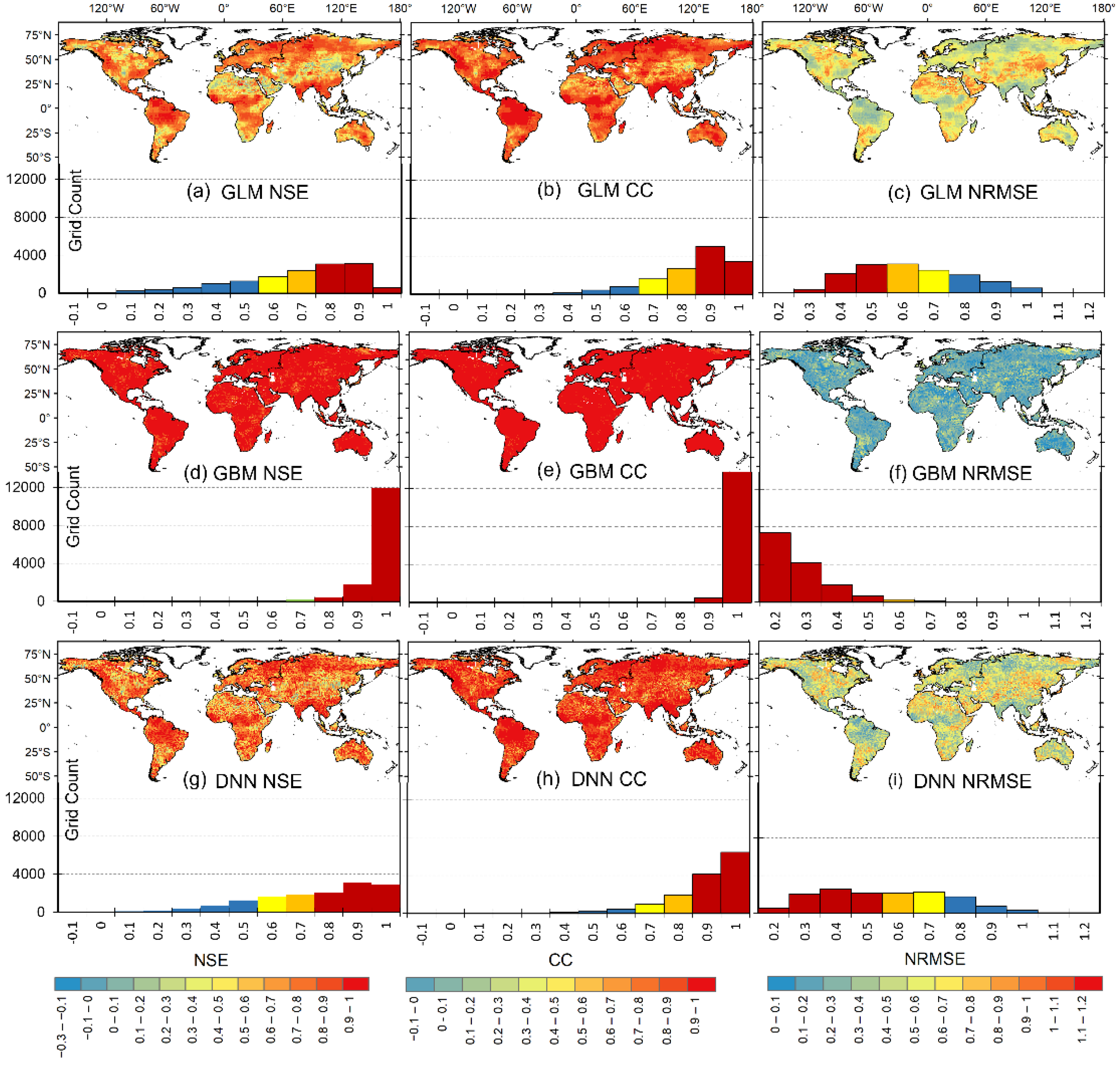
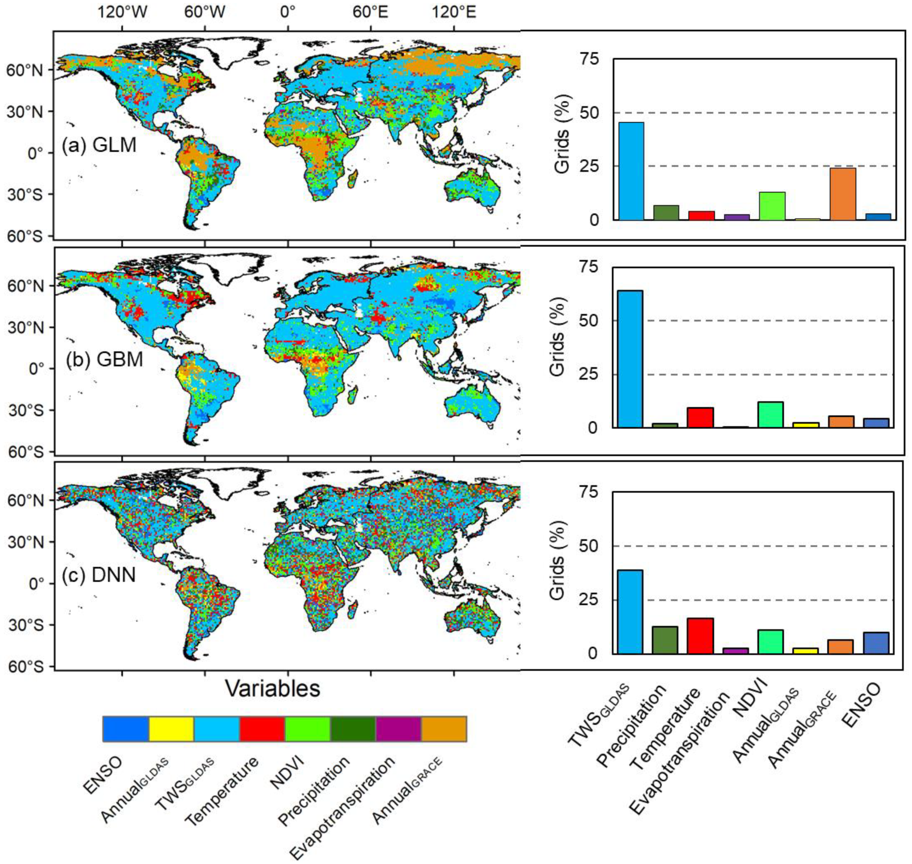
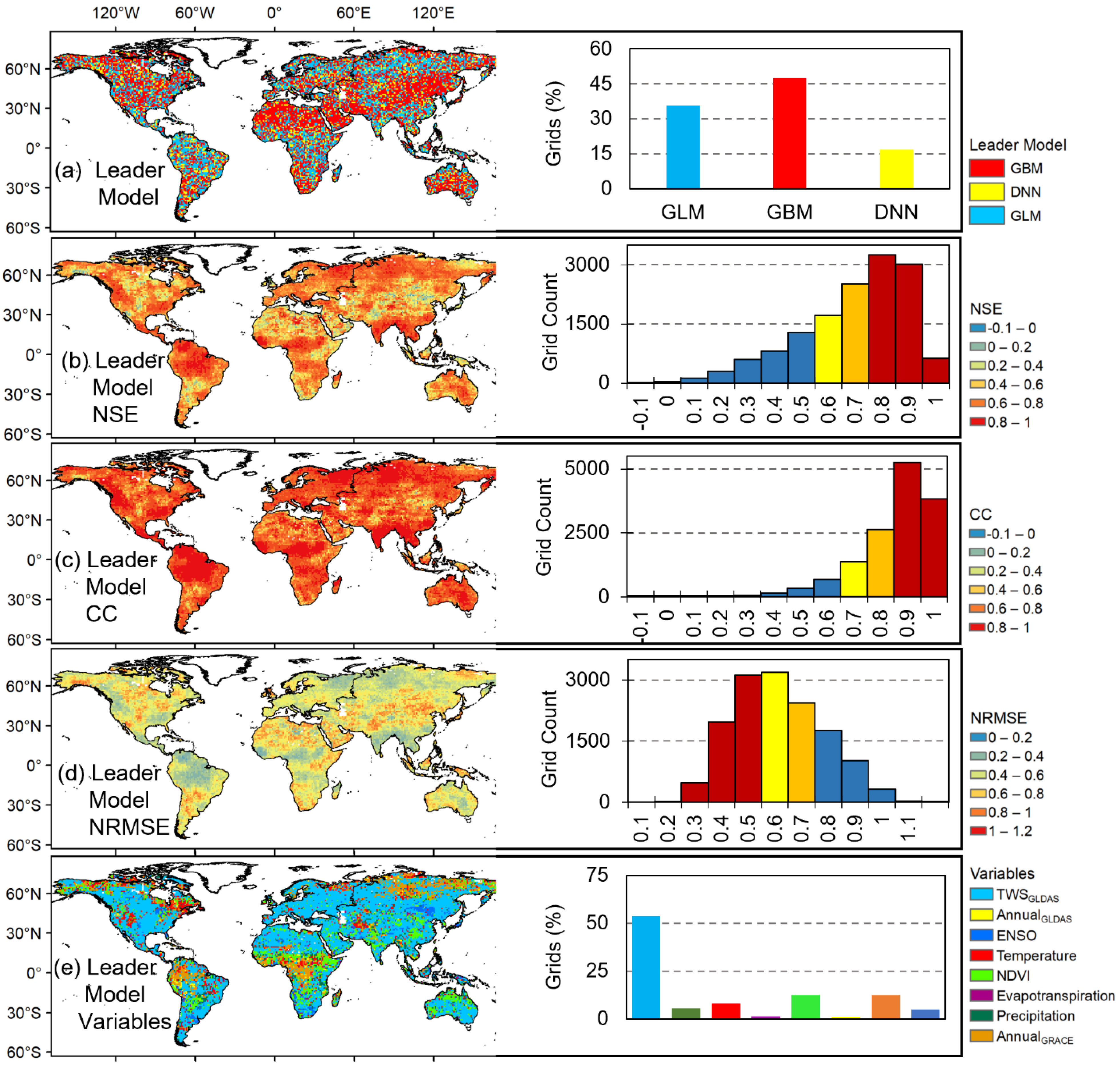
4.1. Model Performance: Grid Scale

Figure 3 shows the spatial distribution of the performance metrics (i.e., NSE, CC, NRMSE) of three models (i.e., GLM, GBM, and DNN) during the testing phase. The average testing performance matrices for grid and basin scales are shown in Table 2. The training performance is shown in Figure A1 (Appendix A). Figure 3 also shows the frequency distribution of each performance metric. Examination of Figure 3 indicates that all models show similar overall patterns of testing performance. Overall, the GLM testing performance has average NSE, CC, and NRMSE values of 0.55 ± 0.26, 0.74 ± 0.19, and 0.63 ± 0.19, respectively (Figure 3a–c, and Table 2). Among the investigated grids (total: 14,310), the GLM shows a very good performance for 29%, good performance for 19%, satisfactory performance for 17%, and poor performance for 35% of the grid cells (Figure 4a). The GBM average performance values for the NSE, CC, and NRMSE are estimated to be 0.59 ± 0.23, 0.77 ± 0.15, and 0.61 ± 0.17, respectively (Figure 3d–f, and Table 2). The GBM model performance is very good, good, satisfactory, and poor for 31%, 22%, 18%, and 29% of total grid cells, respectively (Figure 4a). Overall, the average performance of DNNs were lower than those of the GLMs and GBMs with average NSE, CC, and NRMSE values of 0.49 ± 0.28, 0.73 ± 0.19, and 0.68 ± 0.19, respectively (Figure 3g–i, and Table 2). The DNN model performance is very good for 21%, good for 18%, satisfactory for 27%, and poor for 44% of the total investigated grids (Figure 4a).
Model performance was found to vary spatially. As indicated by the higher NSE testing values, all models have relatively better performance in relatively wet/humid regions such as the Amazon, South Asia, Central Africa, Southeastern United States, and Eastern Europe (Figure 1 and Figure 3a,d,g). The CC and NRMSE for all models also show a similar spatial pattern, with better performance in humid regions (Figure 1 and Figure 3b,c,e,f,h,i). On the other hand, the performance of all models is relatively poor in arid, semi-arid, and highly irrigated regions (Figure 1 and Figure A3). Lower NSE and CC and higher NRMSE values are found to be concentrated over the Sahara Desert, Arabian Peninsula, Northwest China, and the southern part of South America (Figure 3).
The input variables were found to have different impacts on model performance in different grids. We conducted a sensitivity analysis by evaluating the contribution of each input variable to the model performance. The spatial distribution of variables that are the most important is shown in Figure 5. The TWSGLDAS was found to be the most important variable in 45%, 64%, and 39% of all grid points simulated by the GLMs, GBM, and DNN models, respectively. The second and third-most important variables were AnnualGRACE (24%) and NDVI (13%), respectively, for the GLM; NDVI (12%) and temperature (9%), respectively, for the GBM; and temperature (16%) and rainfall (11%), respectively, for the DNN.
Because model performance varies by grid location (Figure 3), a leader model (e.g., the best of the three models) was selected for each grid based on the best NSE value for testing results (Figure 6a). The GBM model was the leader for 47% of the examined grid cells, whereas the GLM and DNN were the leaders for 36% and 17%, respectively. The leader model performance average NSE, CC, and NRMSE are 0.65 ± 0.20, 0.81 ± 0.13, and 0.56 ± 0.16, respectively (Figure 6b–d, and Table 2).
The performance of the leader model is very good for 39%, good for 22%, satisfactory for 17%, and poor for 22% of the total investigated grids (Figure 4a). The leader model performance is significantly higher than that of any of the three individual models, particularly in the very good and poor classes (Figure 4a). In addition, the top three most important input variables for the leader model in each grid were found to be TWSGLDAS (54%), AnnualGRACE (12%), and NDVI (12%) (Figure 6e).

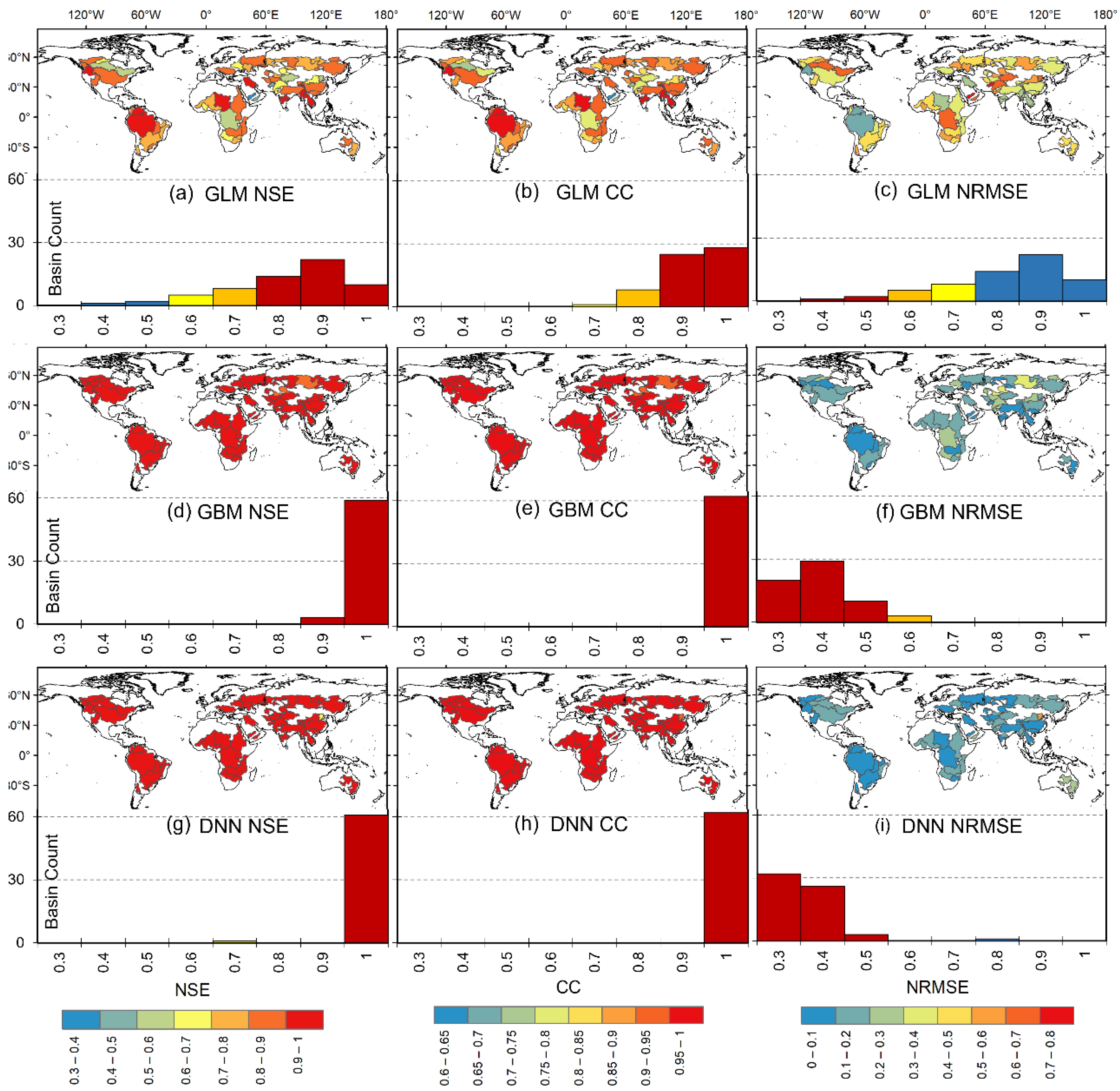
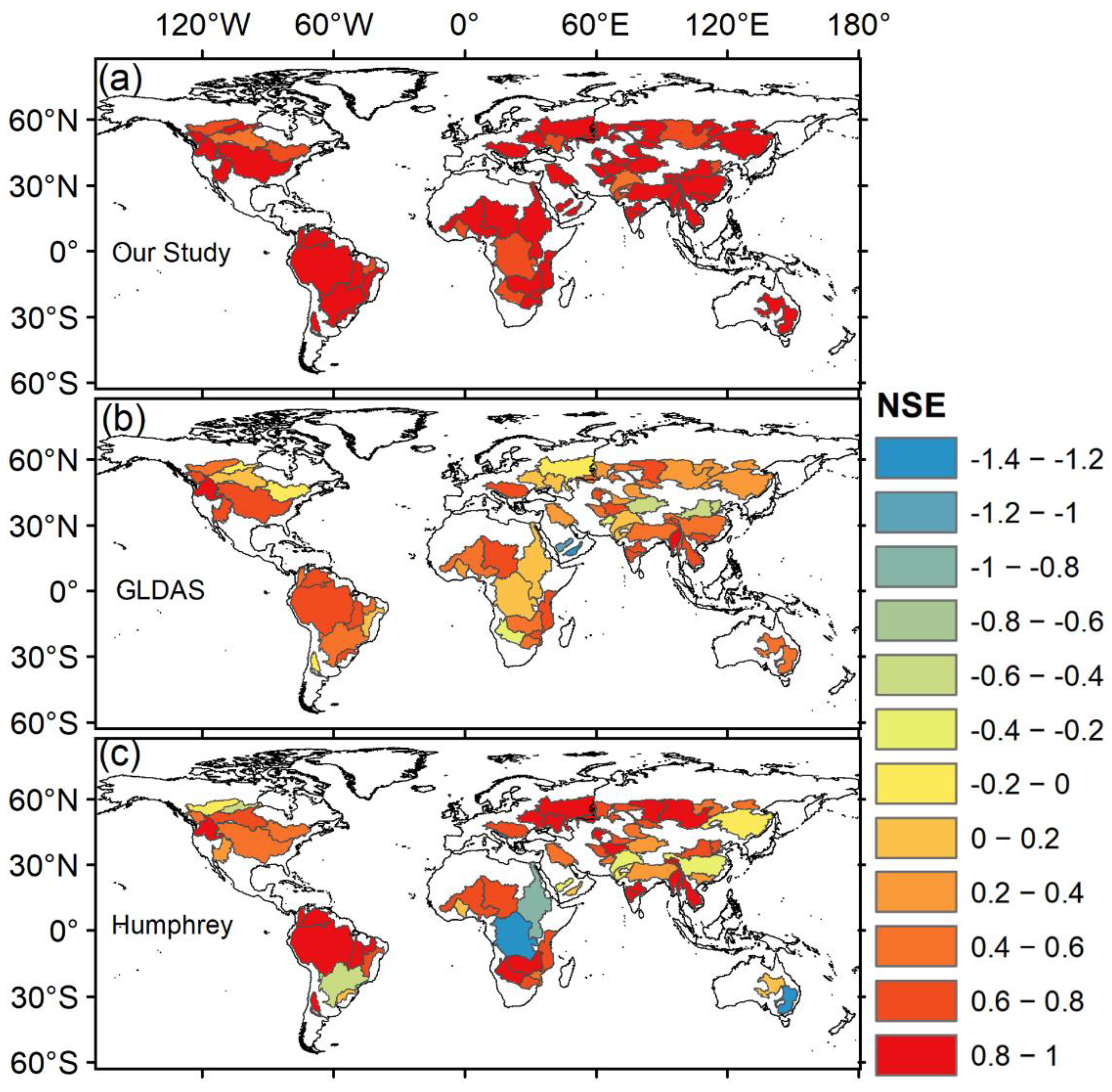
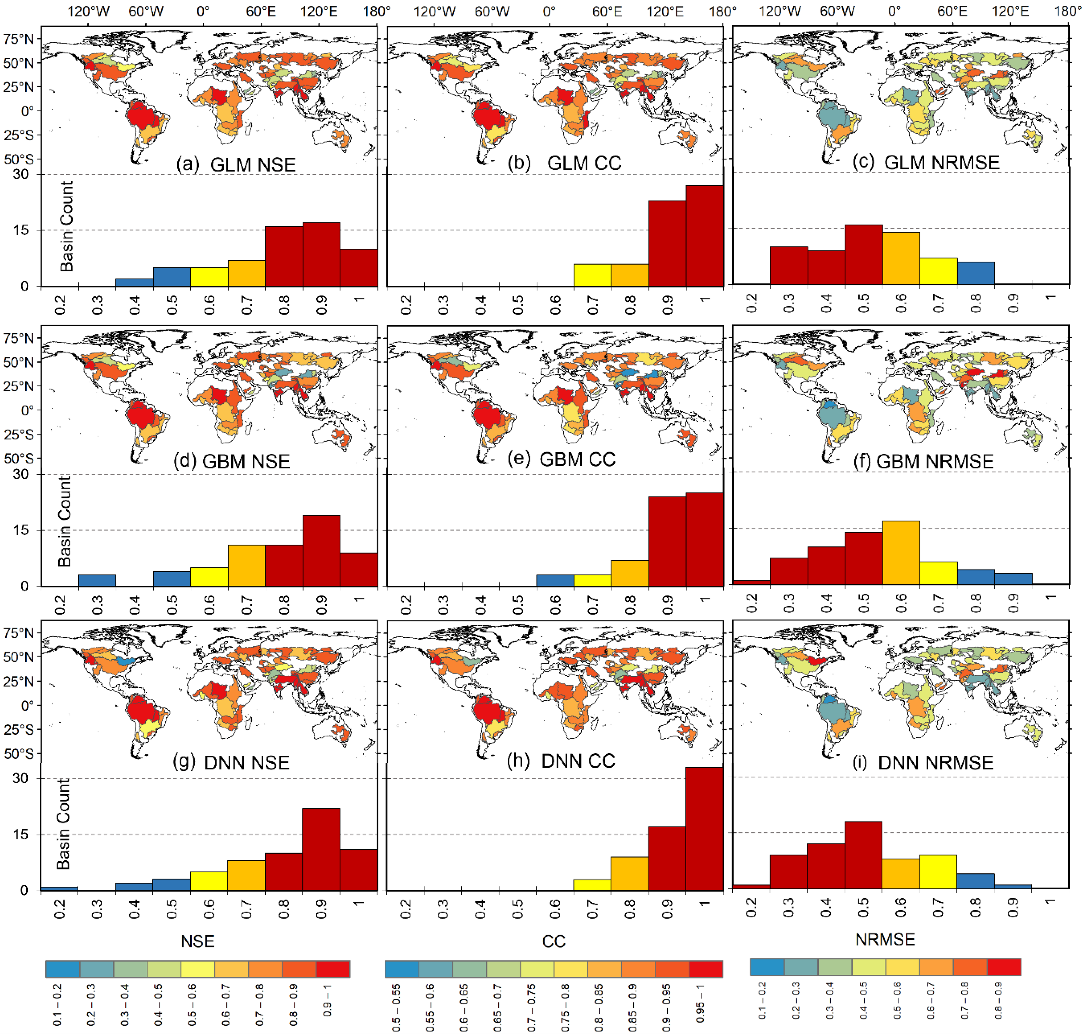
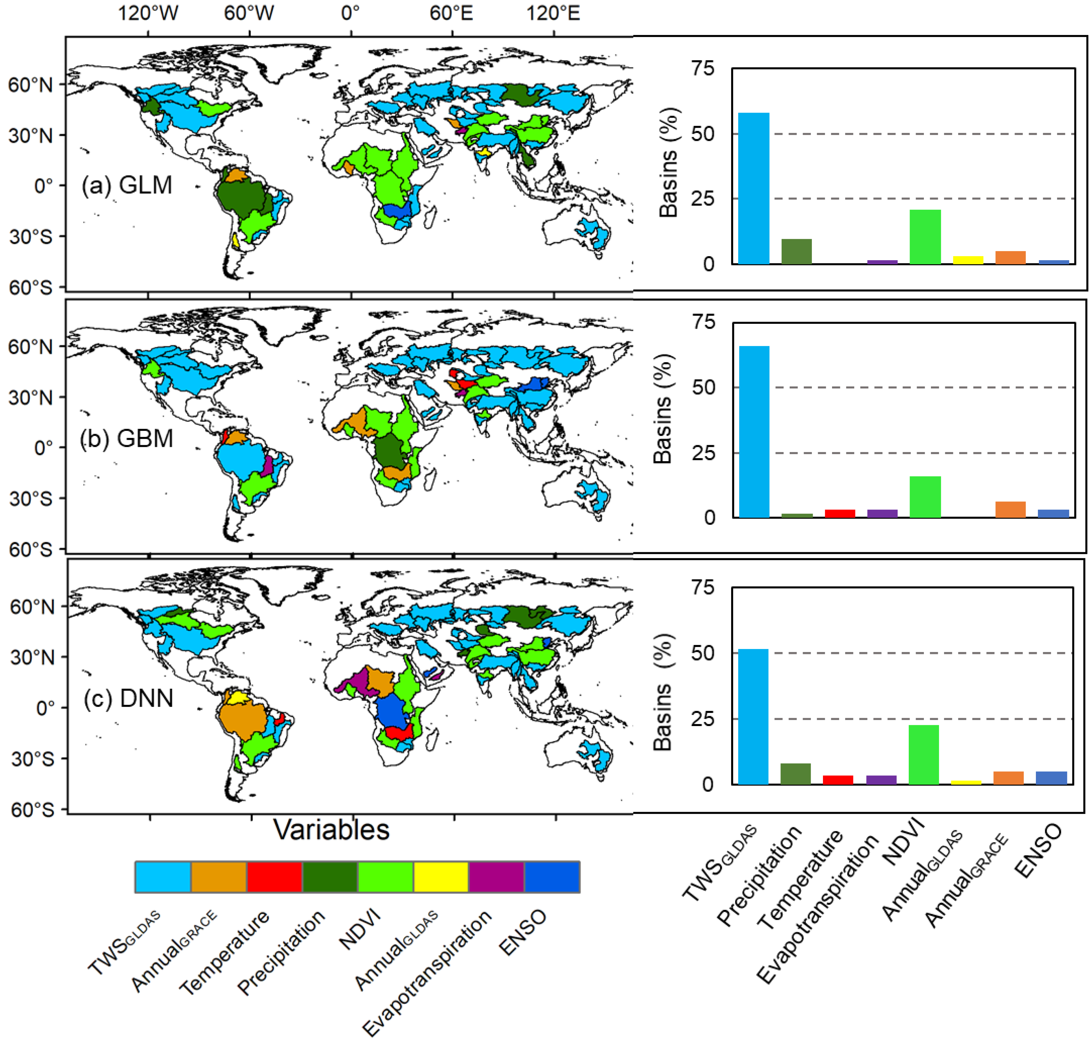
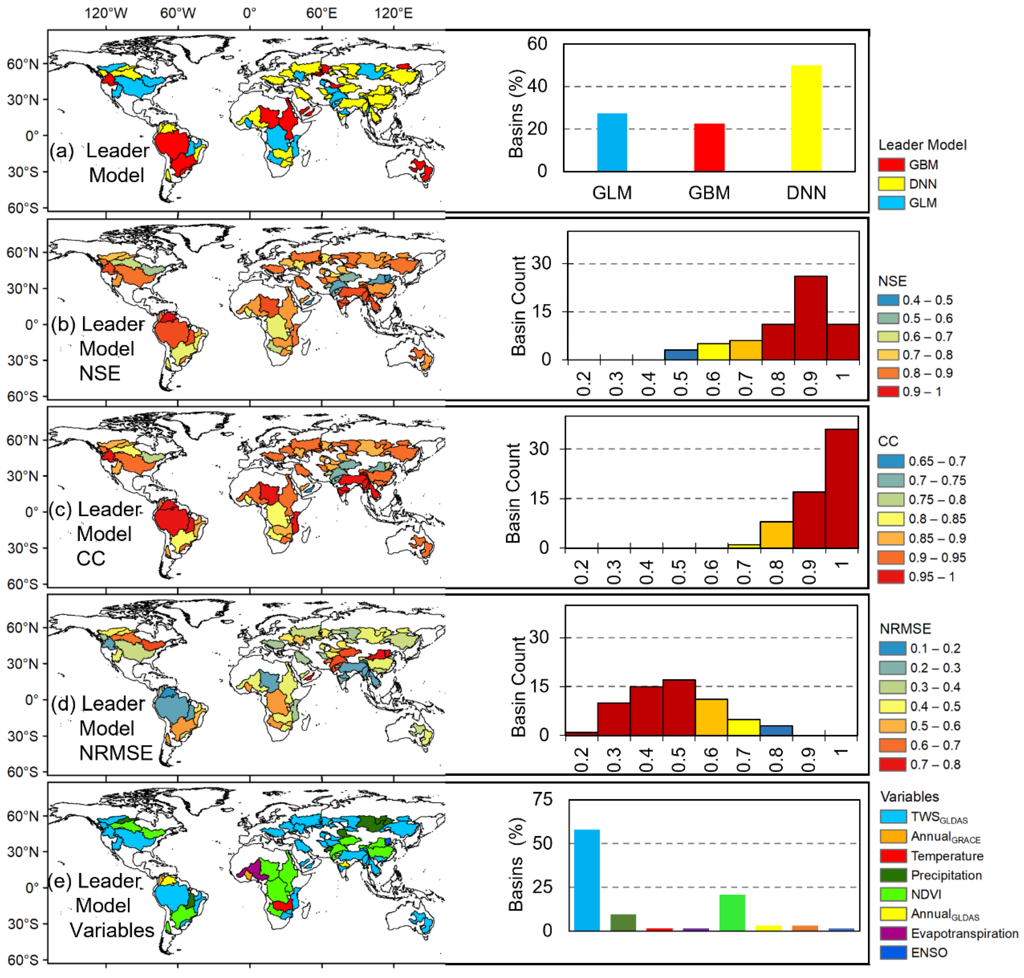
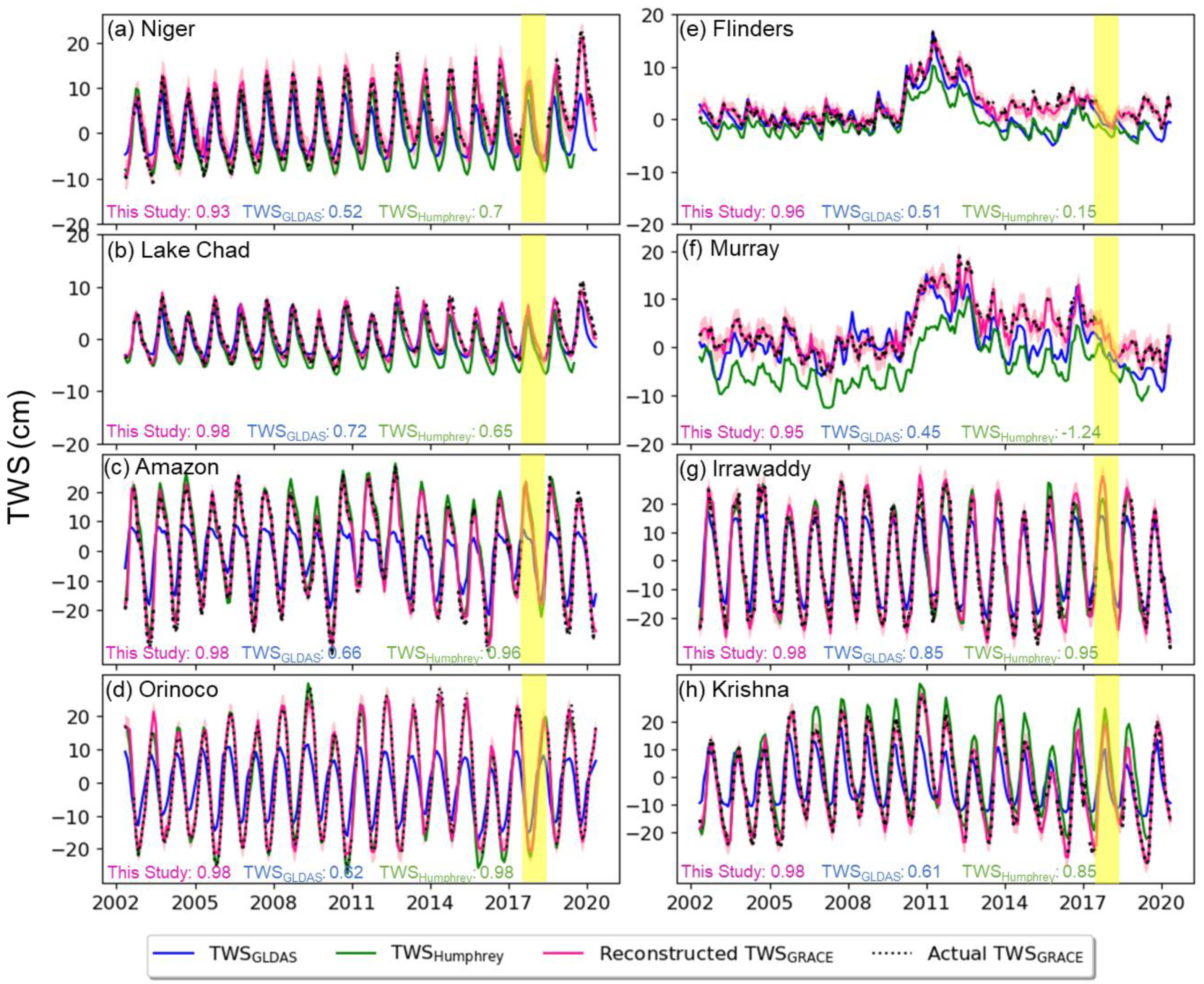
4.2. Model Performance: Basin Scale

Figure 7 and Figure A2 show the spatial distribution of the performance metrics over these 62 global watersheds during the testing and training phases, respectively. For the GLM, the average testing performance is estimated to be 0.74 ± 0.15, 0.87 ± 0.09, and 0.48 ± 0.15 for the NSE, CC, and NRMSE, respectively (Figure 7a–c, and Table 2). The GLM performance is very good for 58% of the basins (Figure 4b), particularly the Amazon, Godawari, Orinoco, Columbia, Irrawaddy, Tocantins, Salween, Irrawaddy, Krishna, and Mekong basins (e.g., Amazon: NSE = 0.95, CC = 0.98, NRMSE = 0.22) and good for 21%, satisfactory for 11%, and poor for 10% of the investigated basins (e.g., Saudi Arabia [NSE = 0.37, CC = 0.78, NRMSE = 0.62], Tarim, Yodo, Hwang Ho, Helmand, and Yemen; Figure 7a–c).
The GBM model’s general performance is estimated to be NSE = 0.73 ± 0.17, CC = 0.85 ± 0.11, NRMSE = 0.49 ± 0.16 (Figure 7d–f, and Table 2). The performance of GBM is very good for 53% of the investigated basins (e.g., Orinoco [NSE = 0.96, CC = 0.98, NRMSE = 0.19], Lake Chad, Columbia, Amazon, Godavari, Mekong, Don, and Ural), good for 26%, and satisfactory for 10% of the investigated basins (Figure 4b). The performance of GBM, however, is poor for 11% of the basins, including Tarim (NSE = 0.25, CC = 0.5, NRMSE = 0.86), Yodo, Hwang Ho, Indus, Narmada, and Yemen. The DNN’s model average performance was estimated to be 0.75 ± 0.17, 0.88 ± 0.09, and 0.46 ± 0.16 for NSE, CC, and NRMSE, respectively (Figure 7g–i and Table 2). The DNN model performance is very good for 65%, good for 14%, satisfactory for 13%, and poor for 8% of the investigated basins (Figure 4b). In particular, the performance of DNN is very good for basins such as Orinoco (NSE = 0.97, CC = 0.99, NRMSE = 0.17), Columbia, Amazon, Tocantins, Ganges-Brahmaputra, Godavari, Si, Irrawaddy, and Mekong and poor for the St. Lawrence (NSE = 0.19, CC = 0.63, NRMSE = 0.89), Yodo, Hwang Ho, Indus, and Yemen basins.
For all three models, TWSGLDAS is the most important variable for most basins (Figure 8). Out of the 62 basins, TWSGLDAS was the most important variable for 58%, 66%, and 52% of the basins for the GLMs (Figure 8a), GBM models (Figure 8b), and DNN models (Figure 8c), respectively. Of all the basins, the NDVI is the second-most important variable for 21% for GLMs, 16% for GBM models, and 23% for DNN models, respectively. Precipitation is the third-most important variable for the GLMs and DNN models with 10% and 8% of the basins, respectively, while AnnualGRACE for the GBM (6% basins).
Based on the testing performance measures, the DNN model outperforms the GBM and GLM models in most of the examined basins (Figure 9a). Thus, it is selected as a leader model for 31 (50%) of the investigated basins. On the other hand, the GBM and GLM are the leader models in 14 (23%) and 17 (27%) basins, respectively. The leader model’s performance is significantly higher than that of any of the individual models. The leader model average performance NSE, CC, and NRMSE values are 0.78 ± 0.14, 0.89 ± 0.07, and 0.43 ± 0.14, respectively (Figure 9b–d). Overall, the performance of the leader model is very good, good, satisfactory, and poor for 71%, 16%, 8%, and 5% of the investigated basins, respectively (Figure 4b). Overall, TWSGLDAS, NDVI, and precipitation are the most important variables for 58%, 21%, and 10% of the basins simulated by the leader model, respectively (Figure 9e).

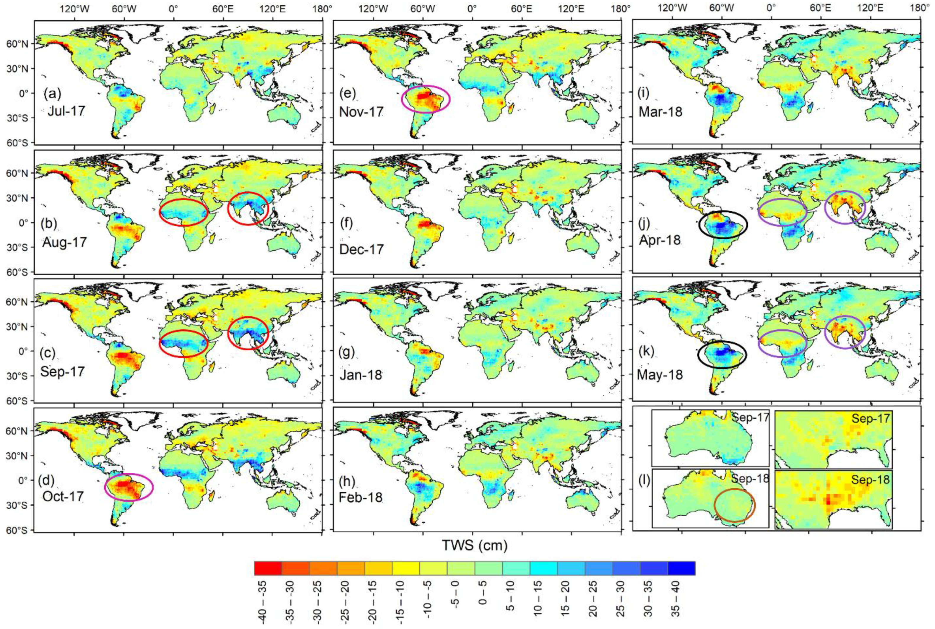
4.3. TWSGRACE Reconstruction Results

To evaluate the TWSGRACE reconstruction results, eight basins were selected as representative examples of different climatic and hydrologic settings across the globe (Figure 10). The TWSGRACE time series derived from the leader model is shown during training, testing, and forecasting (e.g., gap filling) phases. The root-mean-square error for testing phase was plotted as an error bar for the reconstructed TWSGRACE time series. The leader model did an excellent job of reconstructing the TWSGRACE data. Inspection of Figure 10 reveals a better match of the reconstructed TWSGRACE with the actual TWSGRACE compared to that between actual TWSGRACE and TWSGLDAS. The NSE values between the reconstructed and the actual TWSGRACE records are higher (minimum: 0.93; maximum: 0.98) compared to those between TWSGLDAS and actual TWSGRACE records (minimum: 0.45; maximum: 0.85). Figure A4 (Appendix A) shows higher NSE values between the reconstructed and the actual TWSGRACE records compared to those between TWSGLDAS and actual TWSGRACE records for all of the examined 62 basins. The leader model was able to learn and capture the biases between the TWSGRACE and TWSGLDAS. In addition, the leader model accurately captured seasonal variations in TWSGRACE in each of the investigated basins.
Comparison of this study’s reconstructed TWSGRACE results and those produced by Humphrey and Gudmundsson [66] ((TWSHumphry; Figure 10) indicate a better agreement with the observed TWSGRACE of the former. The current study’s reported NSE values between the reconstructed and actual TWSGRACE records are higher (minimum: 0.93; maximum: 0.98) than those derived by TWSHumphry and actual TWSGRACE records (minimum: −1.24; maximum: 0.98). The same pattern is observed over the entire 62 basins (Figure A4) revealing the improved performance by this study’s approach at reconstructing the TWSGRACE trends that are missing from that generated by TWSHumphry.
Inspection of the reconstructed TWSGRACE data during the gap period (July 2017–May 2018) indicates that the grid-scale reconstructed TWSGRACE was also able to capture the August–September high (Figure 11b,c) and the April–May low (Figure 11j,k) TWSGRACE records in South Asia and Central Africa. The April–May high (Figure 11j,k) and October–November low (Figure 11d,e) TWSGRACE records in the Amazon region are also well represented. Furthermore, the reconstructed TWSGRACE reveals a clear response to many climate extremes that occurred during the data gap period. For example, the 2018 Australian drought [123] was captured at both the basin scale (Flinders and Murray basins; Figure 10e,f) and the grid scale (Figure 11l) reconstructed TWSGRACE. Figure 11l shows reconstructed TWSGRACE data over Australia during September 2017 (top left corner) and September 2018 (bottom left corner); the reconstructed TWSGRACE record was lower in 2018 compared to 2017. In the United States, the hurricane season was extremely active in 2017, with four category-three or higher hurricanes that made landfall [124]. The reconstructed TWSGRACE captures the effects of Hurricanes Harvey and Irma (August–September 2017, in the Gulf of Mexico coastal area; Figure 11l), as indicated by the higher TWSGRACE record observed during September 2017 compared to that observed in September 2018.

5. Discussion

The employed models (GLM, GBM, and DNN) perform well in the majority of the investigated basins and grid cells. However, no single model performed exceptionally everywhere. The three models show similar spatial patterns in their performance. Similarity in the spatial variability of all models’ (e.g., GLM, GBM, and DNN) performance during both training and testing phases might be related to the use of a larger set of model inputs. The discrepancies in the performance measures between different models, as indicated by relatively small ranges of NSE, CC, and NRMSE, are expected because these models have different theories, algorithms, assumptions, and principals. The GLM is a standard linear regression model; the DNN and GBM, however, model the nonlinear relationship between the model’s target and inputs. The difference in performance between nonlinear models might also be due to the size of the training and testing sets.
All models indicated a slightly lower performance during the testing phase than in the training phase. The relatively small decline in testing performance may be due to the relatively short number of the training samples [42]. In this study only 147 monthly TWSGRACE values were used in the training phase. An additional reason for differences in performance between the training and testing phases could be the diverse temporal patterns in the model inputs and target variables in the testing phase compared to those in the training phase since data points for these phases were selected randomly.
All models show a relatively better (i.e., high NSE, high CC, and low NRMSE) performance in wet regions on both grid (e.g., Amazon region and surroundings, Indochina Peninsula, Central Africa, and the East European Plain) and basin (e.g., Lake Chad, Orinoco, Amazon, Tocantins, Godavari, Salween, Irrawaddy, Krishna, and Mekong) scales. This higher performance can be attributed mainly to the fact that the spatiotemporal variability in TWSGRACE in these regions is controlled mainly by natural interventions. These interventions are well captured in the model input variables (e.g., rainfall, temperature). In addition, the TWSGRACE data show higher signal-to-noise ratios in humid areas.
The three models performed poorly in arid and semi-arid regions such as North Africa, the Arabian Peninsula, and Northwest China at both grid and basin (e.g., basins Tarim, Yodo, Hwang Ho, Indus, Narmada, Yemen, and Saudi Arabia) scales. Anthropogenic activities such as groundwater extraction for irrigation purposes (Figure A3) are known to occur in these regions [125,126]. In these regions the anthropogenic component is expected to represent a larger percentage of the total TWSGRACE when compared to humid/wet areas. None of the model input variables have accounted for the significant impacts of anthropogenic activities (e.g., lowering of TWSGRACE due to groundwater extraction and aquifer storage depletion; changes in land cover/land use). In addition, TWSGRACE signals in arid and semi-arid regions are so small that errors tend to be on par with signal size [13,127,128].
The relatively lower model performance in non-arid regions could be attributed to prolonged (e.g., decadal) climatic cyclicity that is not adequately represented in the model training period such as those reported in Eastern Africa [25], deforestation activities such as those reported in Central Africa [25], or absence of input variables that account for glaciers (e.g., Tibetan Plateau region) and surface water bodies (St. Lawrence basin) in locations where TWSGRACE was reported to be dominated by glacier [129] and surface water [130] variabilities.
The leader model performance is significantly higher than that of any of the individual models (grid scale: NSE = 0.65 ± 0.20, CC = 0.81 ± 0.13, and NRMSE = 0.56 ± 0.16; basin scale NSE = 0.78 ± 0.14, CC = 0.89 ± 0.07, and NRMSE = 0.43 ± 0.14). The spatial distribution of the leader model results indicates that the DNN model outperforms both GLM and GBM on the basin scale, whereas the GBM outperforms on the grid scale. The DNN model was selected as a leader model for 50% of the examined basins (NSE = 0.75 ± 0.17, CC = 0.88 ± 0.09, and NRMSE = 0.46 ± 0.16). The GBM, on the other hand, was found to be a leader model for 47% of the examined grids (NSE = 0.49 ± 0.28, CC + 0.73 ± 0.19, and NRMSE = 0.68 ± 0.19).
The performance of the basin-scale leader model is higher than that of the grid scale (in 58 basins). In addition, statistical measures of the basin scale reconstructions (e.g., average all of the model input and target variables) were higher (NSE = 0.78 ± 0.14, CC = 0.89 ± 0.07, and NRMSE = 0.43 ± 0.14) compared to those estimated by averaging the grid-scale outputs over each of the investigated basins (NSE = 0.67 ± 0.12, CC = 0.82 ± 0.07, NRMSE = 0.55 ± 0.1). This could be because both input and target variables averaged over basins with large spatial extent are smooth compared to the 1° grid scale [1].
Generally, the GBM tends to outperform the GLMs and DNN models in arid regions such as North Africa, Arabian Peninsula, and Central Asia. This could be related to the GBM’s enhanced ability to predict the complex and nonlinear relationship between target and input variables. The GLM, however, works better in wet regions such as the Amazon, Central Africa, Indochina Peninsula, and the East European Plain. A possible explanation is the linear relationship between input variables and the TWSGRACE in those regions. The DNN model was found to be the leader for all other areas.
The contribution of input variables varies greatly among the three models on both grid and basin scales. Spatially, AnnualGRACE has a greater contribution in humid regions such as the Amazon, Central Africa, and northern Asia. The temperature plays a significant role in model performance in the eastern United States. On the other hand, TWSGLDAS has a significant contribution everywhere. The dominant role of the TWSGLDAS as a controlling factor could be because precipitation and temperature are already captured in the physics of the GLDAS model.
In addition to identifying the leader model as well as input variables that significantly control TWSGRACE variability at each basin and grid point, this study provides better performance compared to some of the previous studies (Table 3). Out of the 28 published studies that used machine learning and statistical techniques to reconstruct TWSGRACE data, this study’s performance metrics were better than 61% and fair when compared to 21% of them. This is a conservative estimate since the performance of the grid-scale outputs in this study was compared to the other studies’ basin-scale outputs. The latter is expected to have higher performance as explained above.
As with other studies, there are multiple sources of uncertainties associated with the TWSGRACE reconstruction herein. These include uncertainties in target (e.g., TWSGRACE) and input variables (e.g., rainfall, temperature, evapotranspiration, TWSGLDAS, NDVI, ENSO, AnnualGRACE, and AnnualGLDAS). Errors in TWSGRACE data include both measurements and leakage errors [131]. Both of these errors were reduced through the precise parameterization of the gravity field solutions and applications of coastlines filters and scaling factors [110]. Uncertainties in model inputs could be propagated from the training phase to the testing phase during the modelling process. These uncertainties were addressed by reporting of the average ± a standard deviation of the performance measures (Section 4.1 and Section 4.2) and errors in the reconstructed TWSGRACE values (Figure 10). Other sources of uncertainties in the reconstructed TWSGRACE data include unmolded human activities (e.g., irrigation, groundwater extraction, land use/land cover changes, etc.) that are challenging to find on a global grid scale. In addition, hyperparameters tuning for the employed models (GLM, GBM, and DNN) is challenging and time-consuming task especially when it comes to simulating a total of 14,310 global grid points. Unoptimized parameters, in some regions, might also introduce errors in the reconstructed TWSGRACE estimates.
The developed approach is robust, effective, and advantageous. Unlike the previous studies [32,71] that used similar data-driven and machine learning techniques, our approach defines the leader model for each basin and grid point. The leader model as well as input variables that significantly control TWSGRACE variability, were globally quantified, for both basin and grid scales, previously performed only for the conterminous United States [42]. This study’s approach offers the capability to reconstruct the TWSGRACE data over small basins and grids (1° × 1°) with high accuracy. Therefore, it helps overcome a limitation that hinders the application of gravimetric datasets (e.g., SLR and Swarm) to small-scale regions given their coarse spatial resolution [42]. When compared to data assimilation techniques [82,83,86] that utilize computationally extensive complex algorithms, the approach herein is computationally efficient and can be utilized on regular computers.

6. Conclusions

This study reviewed the different approaches available in the literature to reconstruct and fill temporal gaps in the TWSGRACE record. The study also provided a new approach to fill current gaps in the TWSGRACE record (20 months), between the GRACE and GRACE-FO missions (11 months), and within the GRACE-FO record (2 months) from April 2002 through to April 2020. The proposed approach compared the performance of three machine learning models (GLM, GBM, and DNN) in reconstructing the TWSGRACE data at both grid (1° × 1°; total: 14,310) and basin (62 global watersheds) scales. Eight variables were used to reconstruct the TWSGRACE data. The model performance was assessed during the training and testing phases using three statistical measures (e.g., NSE, CC, and NRMSE) and a leader model, that showed the highest statistical performance during the testing phase, was selected for each grid and basin. The relative importance of each of the input variables was also investigated.
Results indicate that the leader model reconstructed the TWSGRACE with high accuracy over both grid and local scales, particularly in wet regions and those with low anthropogenic impacts. The reconstructed TWSGRACE data captured extreme climatic events over the investigated basins and grid cells. However, no single model could be used in reconstructing the TWSGRACE over all grids or basins and a combination of models is recommended. Despite the effectiveness of the developed approach, the adopted models exhibit a relatively poor performance in arid and semi-arid regions because they do not incorporate anthropogenic activities as model inputs. This may also be the result of lower signal-to-noise ratio of the TWSGRACE in arid versus humid regions.
According to the most recent National Academy of Sciences Decadal Survey for Earth Science and Applications from Space [132], mass change “within and between the Earth’s atmosphere, oceans, groundwater, and ice sheets” has been recognized as an essential part of observing the Earth system and recognized as a “Designated Observable.” While the Decadal Survey emphasized the importance of measuring mass continuity changes, it is still possible that the GRACE-FO mission, which was designed to have a nominal life of 5 years (2018–2023), could fail prior to the launch of the next mass-change observing system, for which a target launch date has not yet been set. Therefore, there is a fundamental need to predict and/or infer mass change from other variables, even beyond the current gaps.
The developed approach can serve as a reference tool to fill TWSGRACE data gaps in GRACE and GRACE-FO missions. The model performance can be improved particularly in arid and semi-arid regions by incorporating the anthropogenic impact variables into the model inputs. In addition, the presented new approach could be used to reconstruct TWSGRACE for the pre-GRACE era. A long-term and uninterrupted TWSGRACE record could also be used to enhance the groundwater monitoring and other hydrological and climatic processes across the globe.

Author Contributions

Conceptualization, M.A. and B.G.; methodology, B.G. and M.A.; software, B.G. and M.A.; validation, B.G. and M.A.; formal analysis and investigation, and data curation, B.G. and M.A.; resources, M.A. and D.M.; writing—original draft preparation, B.G., M.A., D.M. and D.N.W.; writing—review and editing, B.G., M.A., D.M. and D.N.W.; visualization, B.G. and M.A.; supervision, D.M. and M.A.; project administration, B.G. and M.A.; funding acquisition, B.G., M.A. and D.M. All authors have read and agreed to the published version of the manuscript.

Funding

B. Gyawali and D. Murgulet were supported in part Institutional Grant (NA18OAR4170088) to the Texas Sea Grant College Program from the National Sea Grant Office, National Oceanic and Atmospheric Administration, U.S. Department of Commerce, the Centre for Water Supply Studies, and the Department of Physical and Environmental Sciences at Texas A&M University—Corpus Christi (TAMU-CC). M. Ahmed was supported by the Division of Research and Innovation at TAMU-CC (Research Enhancement Grant, Research Equipment and Infrastructure Grant, and Texas Comprehensive Research Funds (grant number: 141403-00020)). The contribution of D. Wiese represents work carried out at the Jet Propulsion Laboratory/California Institute of Technology, under a contract with the National Aeronautics and Space Administration.

Institutional Review Board Statement

Not applicable.

Informed Consent Statement

Not applicable.

Data Availability Statement

Not applicable.

Acknowledgments

The authors would like to thank the editor and reviewers for their constructive comments and suggestions.

Conflicts of Interest
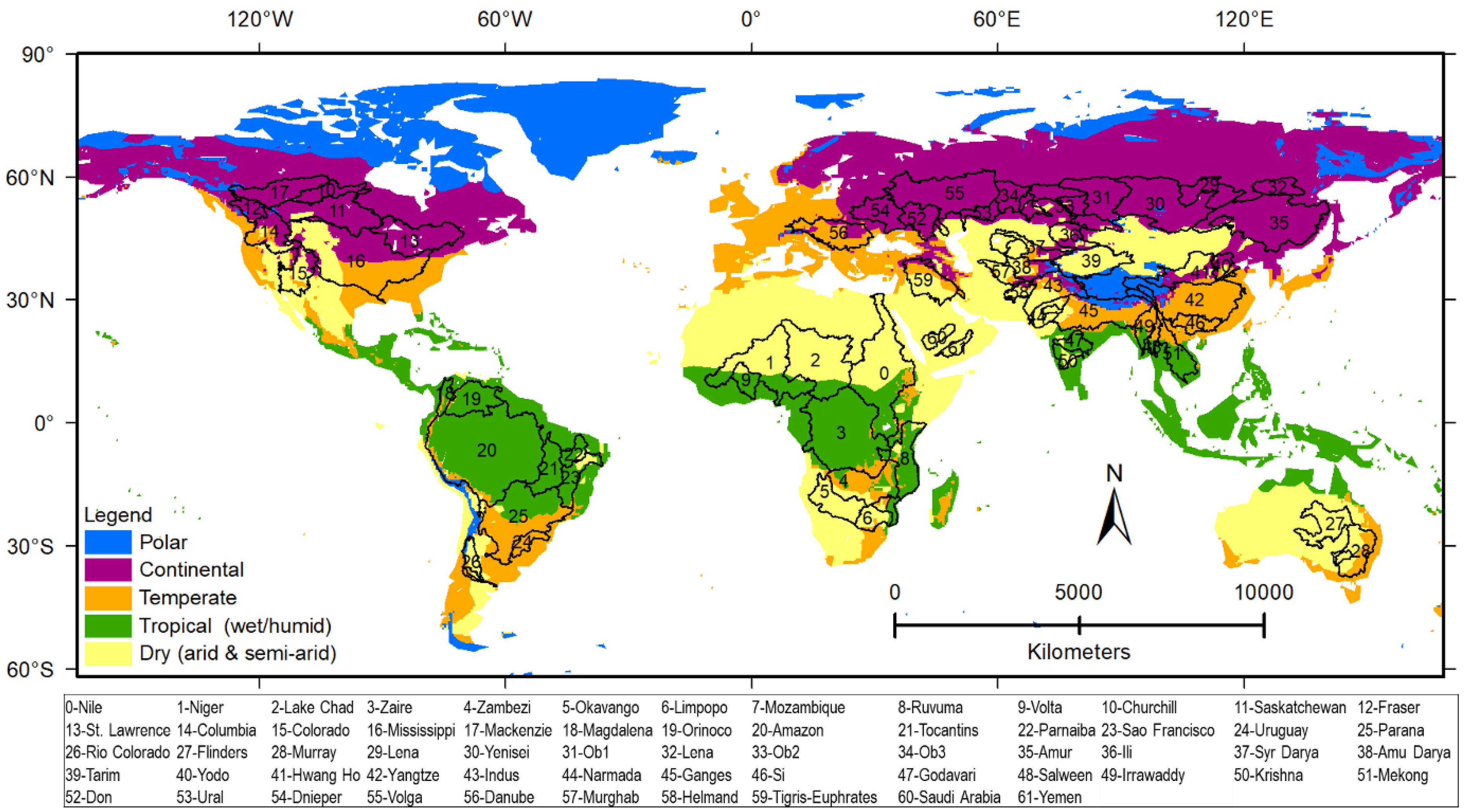
The authors declare no conflict of interest. The funders had no role in the design of the study; in the collection, analyses, or interpretation of data; in the writing of the manuscript, or in the decision to publish the results.

Appendix A

Table A1. Characteristics of global 62 major river basins used in this study.
Basin IDBasin NameContinentPrecipitation (mm/yr)Area
(km2)
Climate Zone
0NileAfrica7043,271,155Dry
1NigerAfrica7042,277,159Dry
2Lake ChadAfrica3962,660,764Dry
3ZaireAfrica15563,735,917Tropical
4ZambeziAfrica9801,472,701Temperate
5OkavangoAfrica561971,144Dry
6LimpopoAfrica537487,829Dry
7Mozambique NE CoastAfrica833278,592Tropical
8RuvumaAfrica10171,071,358Tropical
9VoltaAfrica1016425,491Tropical
10ChurchillNorth America499981,996Continental
11Saskatchewan-NelsonNorth America5482,836,224Continental
12FraserNorth America706620,355Continental
13St. LawrenceNorth America10512,149,625Continental
14ColumbiaNorth America6131,367,203Continental
15ColoradoNorth America320978,636Dry
16MississippiNorth America8845,625,053Temperate/Continental
17MackenzieNorth America4811,992,763Continental
18MagdalenaSouth America2342263,197Tropical
19OrinocoSouth America2374944,775Tropical
20AmazonSouth America22636,025,286Tropical
21TocantinsSouth America1663803,661Tropical
22ParnaibaSouth America1047337,411Tropical
23Sao FranciscoSouth America976673,366Tropical
24UruguaySouth America1795347,840Temperate
25ParanaSouth America13093,065,761Tropical
26Rio ColoradoSouth America332434,140Dry
27FlindersAustralia286971,231Dry
28MurrayAustralia5211,040,403Dry/Temperate
29LenaAsia4571,453,767Continental
30YeniseiAsia4514,177,460Continental
31Ob1Asia6682,221,313Continental
32LenaAsia575898,935Continental
33Ob2Asia5291,681,026Continental
34Ob3Asia560921,174Continental
35AmurAsia6224,776,036Continental
36IliAsia370846,829Continental/Dry
37Syr DaryaAsia387596,945Dry
38Amu DaryaAsia3241,050,574Dry
39Tarim (Yarkand)Asia1121,539,641Dry
40YodoAsia531346,578Continental
41Hwang HoAsia4901,251,658Continental/Dry
42YangtzeAsia10942,584,657Temperate
43IndusAsia5351,202,195dry
44NarmadaAsia409401,453Dry
45Ganges-BrahmaputraAsia12932,001,344Temperate
46SiAsia1502486,550Temperate
47GodavariAsia1165347,993Tropical
48SalweenAsia1113327,489Temperate
49IrrawaddyAsia1802447,888Tropical/Temperate
50KrishnaAsia932280,322Tropical/Dry
51MekongAsia1581871,453Tropical
52DonEurope7221,055,369Continental
53UralEurope489540,152Continental
54DnieperEurope7861,308,031Continental
55VolgaEurope7774,535,995Continental
56DanubeEurope9171,653,884Temperate
57Murghab/Hari RudAsia257465,732Dry
58HelmandEurope241285,431Dry
59Tigris-EuphratesAsia3801,253,767Dry
60Saudi ArabiaAsia80275,525Dry
61YemenAsia66232,406Dry
Figure A1. Spatial (maps) and frequency (bar plots) distributions of the grid-scale training performance for the (ac) GLMs, (df) GBM models, and (gi) DNN models. The color-coded frequency distribution shows the very good (red), good (orange), satisfactory (yellow), and poor (blue) performance categories.
Remotesensing 14 01565 g0a1
Figure A2. Spatial (maps) and frequency (bar plots) distributions of the basin-scale training performance for the (ac) GLMs, (df) GBM models, and (gi) DNN models. The color-coded frequency distribution shows the very good (red), good (orange), satisfactory (yellow), and poor (blue) performance categories.
Remotesensing 14 01565 g0a2
Figure A3. Global map of irrigated areas provided by the Food and Agricultural Organization [133].
Remotesensing 14 01565 g0a3
Figure A4. Basin Scale NSE values between TWSGRACE and this study (a), TWSGLDAS (b), and TWSHumphry (c). The NSE was calculated using data from 2002–2019.
Remotesensing 14 01565 g0a4

References

  1. Tapley, B.D.; Bettadpur, S.; Watkins, M.; Reigber, C. The gravity recovery and climate experiment: Mission overview and early results. Geophys. Res. Lett. 2004, 31, L09607. [Google Scholar] [CrossRef] [Green Version]
  2. Wahr, J.; Molenaar, M.; Bryan, F. Time variability of the earth’s gravity field: Hydrological and oceanic effects and their possible detection using grace. J. Geophys. Res. Solid Earth 1998, 103, 30205–30229. [Google Scholar] [CrossRef]
  3. Ahmed, M.; Sultan, M.; Yan, E.; Wahr, J. Assessing and Improving Land Surface Model Outputs Over Africa Using GRACE, Field, and Remote Sensing Data. Surv. Geophys. 2016, 37, 529–556. [Google Scholar] [CrossRef]
  4. Jacob, T.; Wahr, J.M.; Pfeffer, W.T.; Swenson, S.C. Recent contributions of glaciers and ice caps to sea level rise. Nature 2012, 482, 514–518. [Google Scholar] [CrossRef]
  5. Famiglietti, J.S.; Rodel, M. Water in the balance. Science 2013, 340, 1300–1301. [Google Scholar] [CrossRef] [PubMed]
  6. Han, S.; Riva, R.; Sauber, J.; Okal, E. Source parameter inversion for recent megathrust earthquakes from global gravity field observations. J. Geophys. Res. 2013, 118, 1240–1267. [Google Scholar] [CrossRef] [Green Version]
  7. Ahmed, M.; Abdelmohsen, K. Quantifying Modern Recharge and Depletion Rates of the Nubian Aquifer in Egypt. Surv. Geophys. 2018, 39, 729–751. [Google Scholar] [CrossRef]
  8. Rodell, M.; Famiglietti, J.S.; Wiese, D.N.; Reager, J.T.; Beaudoing, H.K.; Landerer, F.W.; Lo, M.-H. Emerging trends in global freshwater availability. Nature 2018, 557, 651–659. [Google Scholar] [CrossRef] [PubMed]
  9. Yang, C.-S.; Zhang, Q.; Zhao, C.-Y.; Wang, Q.-L.; Ji, L.-Y. Monitoring land subsidence and fault deformation using the small baseline subset InSAR technique: A case study in the Datong Basin, China. J. Geodyn. 2014, 75, 34–40. [Google Scholar] [CrossRef]
  10. Tapley, B.D.; Watkins, M.M.; Flechtner, F.; Reigber, C.; Bettadpur, S.; Rodell, M.; Sasgen, I.; Famiglietti, J.S.; Landerer, F.W.; Chambers, D.P.; et al. Contributions of GRACE to understanding climate change. Nat. Clim. Chang. 2019, 9, 358–369. [Google Scholar] [CrossRef]
  11. Famiglietti, J.S. The global groundwater crisis. Nat. Clim. Change 2014, 4, 945–948. [Google Scholar] [CrossRef]
  12. Gardner, A.S.; Moholdt, G.; Cogley, J.G.; Wouters, B.; Arendt, A.A.; Wahr, J.; Berthier, E.; Hock, R.; Pfeffer, W.T.; Kaser, G.; et al. A Reconciled Estimate of Glacier Contributions to Sea Level Rise: 2003 to 2009. Science 2013, 340, 852–857. [Google Scholar] [CrossRef] [Green Version]
  13. Ahmed, M.; Sultan, M.; Wahr, J.; Yan, E.; Milewski, A.; Sauck, W.; Becker, R.; Welton, B. Integration of GRACE (Gravity Recovery and Climate Experiment) data with traditional data sets for a better understanding of the time-dependent water partitioning in African watersheds. Geology 2011, 39, 479–482. [Google Scholar] [CrossRef] [Green Version]
  14. Ahmed, M.; Wiese, D.N. Short-term trends in africa’s freshwater resources: Rates and drivers. Sci. Total Environ. 2019, 695, 133843. [Google Scholar] [CrossRef] [PubMed]
  15. Niyazi, B.A.; Ahmed, M.; Basahi, J.M.; Masoud, M.Z.; Rashed, M.A. Spatiotemporal trends in freshwater availability in the Red Sea Hills, Saudi Arabia. Arab. J. Geosci. 2018, 11, 702. [Google Scholar] [CrossRef]
  16. Fallatah, O.A.; Ahmed, M.; Cardace, D.; Boving, T.; Akanda, A.S. Assessment of modern recharge to arid region aquifers using an integrated geophysical, geochemical, and remote sensing approach. J. Hydrol. 2019, 569, 600–611. [Google Scholar] [CrossRef]
  17. Fallatah, O.A.; Ahmed, M.; Save, H.; Akanda, A.S. Quantifying temporal variations in water resources of a vulnerable middle eastern transboundary aquifer system. Hydrol. Process. 2017, 31, 4081–4091. [Google Scholar] [CrossRef]
  18. Ahmed, M. Sustainable management scenarios for northern Africa’s fossil aquifer systems. J. Hydrol. 2020, 589, 125196. [Google Scholar] [CrossRef]
  19. Gafurov, A.; Yapiyev, V.; Ahmed, M.; Sagin, J.; Haghighi, E.; Akylbekova, A.; Kløve, B. Groundwater resources. In The Aral Sea Basin, Water for Sustainable Development in Central Asi; Xenarios, S., Schmidt-Vogt, D., Qadir, M., Janusz-Pawletta, B., Abdullaev, I., Eds.; Routledge: London, UK, 2019; pp. 39–51. [Google Scholar]
  20. Gyawali, B.; Murgulet, D.; Ahmed, M. Quantifying changes in groundwater storage and response to hydroclimatic extremes in a coastal aquifer using remote sensing and ground-based measurements: The Texas gulf coast aquifer. Remote Sens. 2022, 14, 612. [Google Scholar] [CrossRef]
  21. Ahmed, M.; Aqnouy, M.; El Messari, J.S. Sustainability of Morocco’s groundwater resources in response to natural and anthropogenic forces. J. Hydrol. 2021, 603, 126866. [Google Scholar] [CrossRef]
  22. Landerer, F.W.; Flechtner, F.M.; Save, H.; Webb, F.H.; Bandikova, T.; Bertiger, W.I.; Bettadpur, S.V.; Byun, S.H.; Dahle, C.; Dobslaw, H.; et al. Extending the Global Mass Change Data Record: GRACE Follow-On Instrument and Science Data Performance. Geophys. Res. Lett. 2020, 47, e2020GL088306. [Google Scholar] [CrossRef]
  23. Gould, P.G.; Koehler, A.B.; Ord, J.K.; Snyder, R.; Hyndman, R.; Vahid-Araghi, F. Forecasting time series with multiple seasonal patterns. Eur. J. Oper. Res. 2008, 191, 207–222. [Google Scholar] [CrossRef]
  24. Mwale, F.D.; Adeloye, A.; Rustum, R. Infilling of missing rainfall and streamflow data in the shire river basin, Malawi–A self organizing map approach. Phys. Chem. Earth Parts A/B/C 2012, 50, 34–43. [Google Scholar] [CrossRef]
  25. Ahmed, M.; Sultan, M.; Elbayoumi, T.; Tissot, P. Forecasting GRACE Data over the African Watersheds Using Artificial Neural Networks. Remote Sens. 2019, 11, 1769. [Google Scholar] [CrossRef] [Green Version]
  26. Ng, W.; Rasmussen, P.; Panu, U. Infilling missing daily precipitation data at multiple sites using a multivariate truncated normal distribution model. Water 2009, 2009, H31D-0813. [Google Scholar]
  27. Tum, M.; Günther, K.P.; Böttcher, M.; Baret, F.; Bittner, M.; Brockmann, C.; Weiss, M. Global Gap-Free MERIS LAI Time Series (2002–2012). Remote Sens. 2016, 8, 69. [Google Scholar] [CrossRef] [Green Version]
  28. Chen, X.; Jiang, J.; Li, H. Drought and Flood Monitoring of the Liao River Basin in Northeast China Using Extended GRACE Data. Remote Sens. 2018, 10, 1168. [Google Scholar] [CrossRef] [Green Version]
  29. Forootan, E.; Kusche, J.; Loth, I.; Schuh, W.-D.; Eicker, A.; Awange, J.; Longuevergne, L.; Diekkrüger, B.; Schmidt, M.; Shum, C.K. Multivariate Prediction of Total Water Storage Changes Over West Africa from Multi-Satellite Data. Surv. Geophys. 2014, 35, 913–940. [Google Scholar] [CrossRef] [Green Version]
  30. Humphrey, V.; Gudmundsson, L.; Seneviratne, S.I. A global reconstruction of climate-driven subdecadal water storage variability. Geophys. Res. Lett. 2017, 44, 2300–2309. [Google Scholar] [CrossRef]
  31. Kenea, T.T.; Kusche, J.; Kebede, S.; Güntner, A. Forecasting terrestrial water storage for drought management in Ethiopia. Hydrol. Sci. J. 2020, 65, 2210–2223. [Google Scholar] [CrossRef]
  32. Li, F.; Kusche, J.; Rietbroek, R.; Wang, Z.; Forootan, E.; Schulze, K.; Lück, C. Comparison of Data-Driven Techniques to Reconstruct (1992–2002) and Predict (2017–2018) GRACE-Like Gridded Total Water Storage Changes Using Climate Inputs. Water Resour. Res. 2020, 56, e2019WR026551. [Google Scholar] [CrossRef] [Green Version]
  33. Long, D.; Shen, Y.; Sun, A.; Hong, Y.; Longuevergne, L.; Yang, Y.; Li, B.; Chen, L. Drought and flood monitoring for a large karst plateau in Southwest China using extended GRACE data. Remote Sens. Environ. 2014, 155, 145–160. [Google Scholar] [CrossRef]
  34. Yin, W.; Hu, L.; Han, S.-C.; Zhang, M.; Teng, Y. Reconstructing Terrestrial Water Storage Variations from 1980 to 2015 in the Beishan Area of China. Geofluids 2019, 2019, 3874742. [Google Scholar] [CrossRef]
  35. De Linage, C.; Famiglietti, J.; Randerson, J. Forecasting terrestrial water storage changes in the amazon basin using atlantic and pacific sea surface temperatures. Hydrol. Earth Syst. Sci. Discuss. 2013, 10, 12453–12483. [Google Scholar]
  36. Pan, M.; Sahoo, A.K.; Troy, T.J.; Vinukollu, R.K.; Sheffield, J.; Wood, A.E.F. Multisource Estimation of Long-Term Terrestrial Water Budget for Major Global River Basins. J. Clim. 2012, 25, 3191–3206. [Google Scholar] [CrossRef]
  37. Li, F.; Kusche, J.; Chao, N.; Wang, Z.; Löcher, A. Long-Term (1979-Present) Total Water Storage Anomalies Over the Global Land Derived by Reconstructing GRACE Data. Geophys. Res. Lett. 2021, 48, e2021GL093492. [Google Scholar] [CrossRef]
  38. Becker, M.; Meyssignac, B.; Xavier, L.; Cazenave, A.; Alkama, R.; Decharme, B. Past terrestrial water storage (1980–2008) in the Amazon Basin reconstructed from GRACE and in situ river gauging data. Hydrol. Earth Syst. Sci. 2011, 15, 533–546. [Google Scholar] [CrossRef] [Green Version]
  39. Hasan, E.; Tarhule, A.; Zume, J.T.; Kirstetter, P.-E. + 50 years of terrestrial hydroclimatic variability in Africa’s transboundary waters. Sci. Rep. 2019, 9, 12327. [Google Scholar] [CrossRef] [PubMed] [Green Version]
  40. Jing, W.; Zhang, P.; Zhao, X.; Yang, Y.; Jiang, H.; Xu, J.; Yang, J.; Li, Y. Extending GRACE terrestrial water storage anomalies by combining the random forest regression and a spatially moving window structure. J. Hydrol. 2020, 590, 125239. [Google Scholar] [CrossRef]
  41. Yang, P.; Xia, J.; Zhan, C.; Wang, T. Reconstruction of terrestrial water storage anomalies in Northwest China during 1948–2002 using GRACE and GLDAS products. Water Policy 2018, 49, 1594–1607. [Google Scholar] [CrossRef] [Green Version]
  42. Sun, A.Y.; Scanlon, B.R.; Save, H.; Rateb, A. Reconstruction of GRACE Total Water Storage Through Automated Machine Learning. Water Resour. Res. 2021, 57, e2020WR028666. [Google Scholar] [CrossRef]
  43. Talpe, M.J.; Nerem, R.S.; Forootan, E.; Lemoine, F.G.; Enderlin, E.M.; Landerer, F.W.; Schmidt, M. Ice mass change in Greenland and Antarctica between 1993 and 2013 from satellite gravity measurements. J. Geod. 2017, 91, 1283–1298. [Google Scholar] [CrossRef] [Green Version]
  44. Löcher, A.; Kusche, J. A hybrid approach for recovering high-resolution temporal gravity fields from satellite laser ranging. J. Geod. 2021, 95, 6. [Google Scholar] [CrossRef]
  45. Loomis, B.D.; Rachlin, K.E.; Luthcke, S.B. Improved Earth Oblateness Rate Reveals Increased Ice Sheet Losses and Mass-Driven Sea Level Rise. Geophys. Res. Lett. 2019, 46, 6910–6917. [Google Scholar] [CrossRef]
  46. Sośnica, K.; Jäggi, A.; Meyer, U.; Thaller, D.; Beutler, G.; Arnold, D.; Dach, R. Time variable Earth’s gravity field from SLR satellites. J. Geod. 2015, 89, 945–960. [Google Scholar] [CrossRef] [Green Version]
  47. Friis-Christensen, E.; Lühr, H.; Hulot, G. Swarm: A constellation to study the Earth’s magnetic field. Earth Planets Space 2006, 58, 351–358. [Google Scholar] [CrossRef] [Green Version]
  48. Forootan, E.; Schumacher, M.; Mehrnegar, N.; Bezděk, A.; Talpe, M.J.; Farzaneh, S.; Zhang, C.; Zhang, Y.; Shum, C.K. An Iterative ICA-Based Reconstruction Method to Produce Consistent Time-Variable Total Water Storage Fields Using GRACE and Swarm Satellite Data. Remote Sens. 2020, 12, 1639. [Google Scholar] [CrossRef]
  49. Meyer, U.; Sosnica, K.; Arnold, D.; Dahle, C.; Thaller, D.; Dach, R.; Jäggi, A. SLR, GRACE and Swarm Gravity Field Determination and Combination. Remote Sens. 2019, 11, 956. [Google Scholar] [CrossRef] [Green Version]
  50. Yi, S.; Sneeuw, N. Filling the Data Gaps Within GRACE Missions Using Singular Spectrum Analysis. J. Geophys. Res. Solid Earth 2021, 126, e2020JB021227. [Google Scholar] [CrossRef]
  51. Velicogna, I.; Wahr, J. Time-variable gravity observations of ice sheet mass balance: Precision and limitations of the GRACE satellite data. Geophys. Res. Lett. 2013, 40, 3055–3063. [Google Scholar] [CrossRef] [Green Version]
  52. Wang, Y. Smoothing Splines: Methods and Applications; CRC Press: Boca Raton, FL, USA, 2011. [Google Scholar]
  53. Li, W.; Wang, W.; Zhang, C.; Wen, H.; Zhong, Y.; Zhu, Y.; Li, Z. Bridging Terrestrial Water Storage Anomaly During GRACE/GRACE-FO Gap Using SSA Method: A Case Study in China. Sensors 2019, 19, 4144. [Google Scholar] [CrossRef] [PubMed] [Green Version]
  54. Wang, F.; Shen, Y.; Chen, T.; Chen, Q.; Li, W. Improved multichannel singular spectrum analysis for post-processing GRACE monthly gravity field models. Geophys. J. Int. 2020, 223, 825–839. [Google Scholar] [CrossRef]
  55. Wang, F.; Shen, Y.; Chen, Q.; Wang, W. Bridging the gap between GRACE and GRACE follow-on monthly gravity field solutions using improved multichannel singular spectrum analysis. J. Hydrol. 2021, 594, 125972. [Google Scholar] [CrossRef]
  56. Vautard, R.; Yiou, P.; Ghil, M. Singular-spectrum analysis: A toolkit for short, noisy chaotic signals. Phys. D Nonlinear Phenom. 1992, 58, 95–126. [Google Scholar] [CrossRef]
  57. Long, D.; Scanlon, B.R.; Longuevergne, L.; Sun, A.Y.; Fernando, D.N.; Save, H. GRACE satellite monitoring of large depletion in water storage in response to the 2011 drought in Texas. Geophys. Res. Lett. 2013, 40, 3395–3401. [Google Scholar] [CrossRef] [Green Version]
  58. Scanlon, B.R.; Zhang, Z.; Save, H.; Sun, A.Y.; Schmied, H.M.; van Beek, L.P.H.; Wiese, D.N.; Wada, Y.; Long, D.; Reedy, R.C.; et al. Global models underestimate large decadal declining and rising water storage trends relative to GRACE satellite data. Proc. Natl. Acad. Sci. 2018, 115, E1080–E1089. [Google Scholar] [CrossRef] [PubMed] [Green Version]
  59. Scanlon, B.R.; Zhang, Z.; Rateb, A.; Sun, A.; Wiese, D.; Save, H.; Beaudoing, H.; Lo, M.H.; Müller-Schmied, H.; Döll, P.; et al. Tracking Seasonal Fluctuations in Land Water Storage Using Global Models and GRACE Satellites. Geophys. Res. Lett. 2019, 46, 5254–5264. [Google Scholar] [CrossRef]
  60. Rodell, M.; Houser, P.R.; Jambor, U.; Gottschalck, J.; Mitchell, K.; Meng, C.-J.; Arsenault, K.; Cosgrove, B.; Radakovich, J.; Bosilovich, M.; et al. The Global Land Data Assimilation System. Bull. Am. Meteorol. Soc. 2004, 85, 381–394. [Google Scholar] [CrossRef] [Green Version]
  61. Oleson, K.W.; Niu, G.-Y.; Yang, Z.-L.; Lawrence, D.; Thornton, P.; Lawrence, P.J.; Stöckli, R.; Dickinson, R.E.; Bonan, G.B.; Levis, S.; et al. Improvements to the Community Land Model and their impact on the hydrological cycle. J. Geophys. Res. 2008, 113, G01021. [Google Scholar] [CrossRef]
  62. Fan, Y.; Van Den Dool, H. Climate Prediction Center global monthly soil moisture data set at 0.5 resolution for 1948 to present. J. Geophys. Res. Earth Surf. 2004, 109, D10102. [Google Scholar] [CrossRef] [Green Version]
  63. Döll, P.; Kaspar, F.; Lehner, B. A global hydrological model for deriving water availability indicators: Model tuning and validation. J. Hydrol. 2003, 270, 105–134. [Google Scholar] [CrossRef]
  64. Zhang, D.; Zhang, Q.; Werner, A.; Liu, X. GRACE-Based Hydrological Drought Evaluation of the Yangtze River Basin, China. J. Hydrometeorol. 2016, 17, 811–828. [Google Scholar] [CrossRef]
  65. Nie, N.; Zhang, W.; Zhang, Z.; Guo, H.; Ishwaran, N. Reconstructed Terrestrial Water Storage Change (ΔTWS) from 1948 to 2012 over the Amazon Basin with the Latest GRACE and GLDAS Products. Water Resour. Manag. 2016, 30, 279–294. [Google Scholar] [CrossRef]
  66. Humphrey, V.; Gudmundsson, L. Grace-rec: A reconstruction of climate-driven water storage changes over the last century, earth syst. Sci. Data 2019, 11, 1153–1170. [Google Scholar] [CrossRef] [Green Version]
  67. Ferreira, V.G.; Andam-Akorful, S.A.; Dannouf, R.; Adu-Afari, E. A Multi-Sourced Data Retrodiction of Remotely Sensed Terrestrial Water Storage Changes for West Africa. Water 2019, 11, 401. [Google Scholar] [CrossRef] [Green Version]
  68. Sun, A.Y.; Scanlon, B.R.; Zhang, Z.; Walling, D.; Bhanja, S.N.; Mukherjee, A.; Zhong, Z. Combining Physically Based Modeling and Deep Learning for Fusing GRACE Satellite Data: Can We Learn From Mismatch? Water Resour. Res. 2019, 55, 1179–1195. [Google Scholar] [CrossRef] [Green Version]
  69. Jing, W.; Di, L.; Zhao, X.; Yao, L.; Xia, X.; Liu, Y.; Yang, J.; Li, Y.; Zhou, C. A data-driven approach to generate past GRACE-like terrestrial water storage solution by calibrating the land surface model simulations. Adv. Water Resour. 2020, 143, 103683. [Google Scholar] [CrossRef]
  70. Zhu, C.; Zhan, W.; Liu, J.; Chen, M. Application of singular spectrum analysis in reconstruction of the annual signal from GRACE. J. Appl. Geod. 2020, 14, 295–302. [Google Scholar] [CrossRef]
  71. Sun, Z.; Long, D.; Yang, W.; Li, X.; Pan, Y. Reconstruction of GRACE Data on Changes in Total Water Storage Over the Global Land Surface and 60 Basins. Water Resour. Res. 2020, 56, e2019WR026250. [Google Scholar] [CrossRef]
  72. Sohoulande, C.D.; Martin, J.; Szogi, A.; Stone, K. Climate-driven prediction of land water storage anomalies: An outlook for water resources monitoring across the conterminous United States. J. Hydrol. 2020, 588, 125053. [Google Scholar] [CrossRef]
  73. Jing, W.; Zhao, X.; Yao, L.; Di, L.; Yang, J.; Li, Y.; Guo, L.; Zhou, C. Can Terrestrial Water Storage Dynamics be Estimated From Climate Anomalies? Earth Space Sci. 2020, 7, e2019EA000959. [Google Scholar] [CrossRef] [Green Version]
  74. Jeon, W.; Kim, J.-S.; Seo, K.-W. Reconstruction of Terrestrial Water Storage of GRACE/GFO Using Convolutional Neural Network and Climate Data. J. Korean Earth Sci. Soc. 2021, 42, 445–458. [Google Scholar] [CrossRef]
  75. Yu, Q.; Wang, S.; He, H.; Yang, K.; Ma, L.; Li, J. Reconstructing GRACE-like TWS anomalies for the Canadian landmass using deep learning and land surface model. Int. J. Appl. Earth Obs. Geoinf. 2021, 102, 102404. [Google Scholar] [CrossRef]
  76. Tang, S.; Wang, H.; Feng, Y.; Liu, Q.; Wang, T.; Liu, W.; Sun, F. Random Forest-Based Reconstruction and Application of the GRACE Terrestrial Water Storage Estimates for the Lancang-Mekong River Basin. Remote Sens. 2021, 13, 4831. [Google Scholar] [CrossRef]
  77. Yang, X.; Tian, S.; You, W.; Jiang, Z. Reconstruction of continuous GRACE/GRACE-FO terrestrial water storage anomalies based on time series decomposition. J. Hydrol. 2021, 603, 127018. [Google Scholar] [CrossRef]
  78. Mo, S.; Zhong, Y.; Forootan, E.; Mehrnegar, N.; Yin, X.; Wu, J.; Feng, W.; Shi, X. Bayesian convolutional neural networks for predicting the terrestrial water storage anomalies during GRACE and GRACE-FO gap. J. Hydrol. 2021, 604, 127244. [Google Scholar] [CrossRef]
  79. Mueller, B.; Hirschi, M.; Seneviratne, S.I. New diagnostic estimates of variations in terrestrial water storage based on ERA-Interim data. Hydrol. Process. 2011, 25, 996–1008. [Google Scholar] [CrossRef]
  80. Eicker, A.; Schumacher, M.; Kusche, J.; Döll, P.; Schmied, H.M. Calibration/Data Assimilation Approach for Integrating GRACE Data into the WaterGAP Global Hydrology Model (WGHM) Using an Ensemble Kalman Filter: First Results. Surv. Geophys. 2014, 35, 1285–1309. [Google Scholar] [CrossRef]
  81. Kumar, S.V.; Zaitchik, B.F.; Peters-Lidard, C.D.; Rodell, M.; Reichle, R.; Li, B.; Jasinski, M.; Mocko, D.; Getirana, A.; De Lannoy, G.; et al. Assimilation of Gridded GRACE Terrestrial Water Storage Estimates in the North American Land Data Assimilation System. J. Hydrometeorol. 2016, 17, 1951–1972. [Google Scholar] [CrossRef]
  82. Girotto, M.; De Lannoy, G.J.M.; Reichle, R.H.; Rodell, M. Assimilation of gridded terrestrial water storage observations from GRACE into a land surface model. Water Resour. Res. 2016, 52, 4164–4183. [Google Scholar] [CrossRef] [Green Version]
  83. Li, B.; Rodell, M.; Kumar, S.; Beaudoing, H.K.; Getirana, A.; Zaitchik, B.F.; De Goncalves, L.G.; Cossetin, C.; Bhanja, S.; Mukherjee, A.; et al. Global GRACE Data Assimilation for Groundwater and Drought Monitoring: Advances and Challenges. Water Resour. Res. 2019, 55, 7564–7586. [Google Scholar] [CrossRef] [Green Version]
  84. Tian, S.; Tregoning, P.; Renzullo, L.J.; Dijk, A.V.; Walker, J.P.; Pauwels, V.; Allgeyer, S. Improved water balance component estimates through joint assimilation of GRACE water storage and SMOS soil moisture retrievals. Water Resour. Res. 2017, 53, 1820–1840. [Google Scholar] [CrossRef]
  85. Tangdamrongsub, N.; Han, S.-C.; Tian, S.; Schmied, H.M.; Sutanudjaja, E.H.; Ran, J.; Feng, W. Evaluation of Groundwater Storage Variations Estimated from GRACE Data Assimilation and State-of-the-Art Land Surface Models in Australia and the North China Plain. Remote Sens. 2018, 10, 483. [Google Scholar] [CrossRef] [Green Version]
  86. Tangdamrongsub, N.; Han, S.-C.; Yeo, I.-Y.; Dong, J.; Steele-Dunne, S.C.; Willgoose, G.; Walker, J.P. Multivariate data assimilation of GRACE, SMOS, SMAP measurements for improved regional soil moisture and groundwater storage estimates. Adv. Water Resour. 2020, 135, 103477. [Google Scholar] [CrossRef]
  87. Khaki, M.; Forootan, E.; Kuhn, M.; Awange, J.; van Dijk, A.I.J.M.; Schumacher, M.; Sharifi, M.A. Determining water storage depletion within Iran by assimilating GRACE data into the W3RA hydrological model. Adv. Water Resour. 2018, 114, 1–18. [Google Scholar] [CrossRef] [Green Version]
  88. Soltani, S.S.; Ataie-Ashtiani, B.; Simmons, C.T. Review of assimilating GRACE terrestrial water storage data into hydrological models: Advances, challenges and opportunities. Earth-Sci. Rev. 2021, 213, 103487. [Google Scholar] [CrossRef]
  89. Nie, W.; Zaitchik, B.F.; Rodell, M.; Kumar, S.V.; Arsenault, K.R.; Li, B.; Getirana, A. Assimilating GRACE Into a Land Surface Model in the Presence of an Irrigation-Induced Groundwater Trend. Water Resour. Res. 2019, 55, 11274–11294. [Google Scholar] [CrossRef]
  90. Hussein, E.A.; Thron, C.; Ghaziasgar, M.; Bagula, A.; Vaccari, M. Groundwater Prediction Using Machine-Learning Tools. Algorithms 2020, 13, 300. [Google Scholar] [CrossRef]
  91. Reager, J.T.; Famiglietti, J.S. Characteristic mega-basin water storage behavior using GRACE. Water Resour. Res. 2013, 49, 3314–3329. [Google Scholar] [CrossRef] [Green Version]
  92. De Linage, C.; Famiglietti, J.S.; Randerson, J.T. Statistical prediction of terrestrial water storage changes in the Amazon Basin using tropical Pacific and North Atlantic sea surface temperature anomalies. Hydrol. Earth Syst. Sci. 2014, 18, 2089–2102. [Google Scholar] [CrossRef] [Green Version]
  93. Kottek, M.; Grieser, J.; Beck, C.; Rudolf, B.; Rubel, F. World map of the Köppen-Geiger climate classification updated. Meteorol. Z. 2006, 15, 259–263. [Google Scholar] [CrossRef]
  94. Dobson, A.J.; Barnett, A. An Introduction to Generalized Linear Models; CRC Press: Boca Raton, FL, USA, 2018. [Google Scholar]
  95. Kuhn, M. Building predictive models in r using the caret package. J. Stat. Softw. 2008, 28, 1–26. [Google Scholar] [CrossRef] [Green Version]
  96. Coxe, S.; West, S.G.; Aiken, L.S. Generalized linear models. Oxf. Handb. Quant. Methods 2013, 2, 26–51. [Google Scholar]
  97. Friedman, J.H. Stochastic gradient boosting. Comput. Stat. Data Anal. 2002, 38, 367–378. [Google Scholar] [CrossRef]
  98. Friedman, J.H. Greedy function approximation: A gradient boosting machine. Ann. Stat. 2001, 29, 1189–1232. [Google Scholar] [CrossRef]
  99. Zhou, J.; Li, E.; Yang, S.; Wang, M.; Shi, X.; Yao, S.; Mitri, H.S. Slope stability prediction for circular mode failure using gradient boosting machine approach based on an updated database of case histories. Saf. Sci. 2019, 118, 505–518. [Google Scholar] [CrossRef]
  100. Breiman, L.; Friedman, J.; Stone, C.J.; Olshen, R.A. Classification and Regression Trees; CRC press: Boca Raton, FL, USA, 1984. [Google Scholar]
  101. Tao, Y.; Gao, X.; Hsu, K.; Sorooshian, S.; Ihler, A. A Deep Neural Network Modeling Framework to Reduce Bias in Satellite Precipitation Products. J. Hydrometeorol. 2016, 17, 931–945. [Google Scholar] [CrossRef]
  102. Goodfellow, I.; Bengio, Y.; Courville, A.; Bengio, Y. Deep Learning; MIT press Cambridge: Cambridge, MA, USA, 2016. [Google Scholar]
  103. Sun, A.Y. Predicting groundwater level changes using GRACE data. Water Resour. Res. 2013, 49, 5900–5912. [Google Scholar] [CrossRef]
  104. Bengio, Y. Learning Deep Architectures for AI; Now Publishers Inc: Delft, The Netherlands, 2009. [Google Scholar]
  105. Guan, K.; Wood, E.F.; Medvigy, D.; Kimball, J.; Pan, M.; Caylor, K.K.; Sheffield, J.; Xu, X.; Jones, M.O. Terrestrial hydrological controls on land surface phenology of African savannas and woodlands. J. Geophys. Res. Biogeosciences 2014, 119, 1652–1669. [Google Scholar] [CrossRef]
  106. Hilker, T.; Lyapustin, A.I.; Tucker, C.J.; Hall, F.G.; Myneni, R.B.; Wang, Y.; Bi, J.; de Moura, Y.M.; Sellers, P.J. Vegetation dynamics and rainfall sensitivity of the Amazon. Proc. Natl. Acad. Sci. USA 2014, 111, 16041–16046. [Google Scholar] [CrossRef] [Green Version]
  107. Scanlon, B.R.; Rateb, A.; Anyamba, A.; Kebede, S.; MacDonald, A.M.; Shamsudduha, M.; Small, I.J.; Sun, A.Y.; Taylor, R.G.; Xie, H. Linkages between GRACE water storage, hydrologic extremes, and climate teleconnections in major African aquifers. Environ. Res. Lett. 2021, 17, 014046. [Google Scholar] [CrossRef]
  108. Frappart, F.; Ramillien, G.; Ronchail, J. Changes in terrestrial water storage versus rainfall and discharges in the Amazon basin. Int. J. Climatol. 2013, 33, 3029–3046. [Google Scholar] [CrossRef] [Green Version]
  109. Watkins, M.M.; Wiese, D.N.; Yuan, D.N.; Boening, C.; Landerer, F.W. Improved methods for observing earth’s time variable mass distribution with grace using spherical cap mascons. J. Geophys. Res. Solid Earth 2015, 120, 2648–2671. [Google Scholar] [CrossRef]
  110. Wiese, D.N.; Landerer, F.W.; Watkins, M.M. Quantifying and reducing leakage errors in the JPL RL05M GRACE mascon solution. Water Resour. Res. 2016, 52, 7490–7502. [Google Scholar] [CrossRef]
  111. Scanlon, B.R.; Zhang, Z.; Save, H.; Wiese, D.N.; Landerer, F.W.; Long, D.; Longuevergne, L.; Chen, J. Global evaluation of new GRACE mascon products for hydrologic applications. Water Resour. Res. 2016, 52, 9412–9429. [Google Scholar] [CrossRef]
  112. Rodell, M.; Houser, P.; Peters-Lidard, C.; Kato, H.; Kumar, S.; Gottschalck, J.; Mitchell, K.; Meng, J. Nasa/Noaa’s global land data assimilation system (GLDAS): Recent results and future plans. In Proceedings of the ECMWF/ELDAS Workshop on Land Surface Assimilation, Shinfield, UK, 8–11 November 2004; pp. 61–68. [Google Scholar]
  113. Ek, M.B.; Mitchell, K.E.; Lin, Y.; Rogers, E.; Grunmann, P.; Koren, V.; Gayno, G.; Tarpley, J.D. Implementation of Noah land surface model advances in the National Centers for Environmental Prediction operational mesoscale Eta model. J. Geophys. Res. Earth Surf. 2003, 108, 8851. [Google Scholar] [CrossRef]
  114. Yang, T.; Wang, C.; Yu, Z.; Xu, F. Characterization of spatio-temporal patterns for various GRACE- and GLDAS-born estimates for changes of global terrestrial water storage. Glob. Planet. Chang. 2013, 109, 30–37. [Google Scholar] [CrossRef]
  115. Huffman, G.J.; Stocker, E.F.; Bolvin, D.T.; Nelkin, E.J.; Tan, J. Gpm Imerg Final Precipitation l3 1 Month 0.1 Degree × 0.1 Degree V06; Goddard Earth Sciences Data and Information Services Center: Greenbelt, MD, USA, 2019. Available online: https://disc.gsfc.nasa.gov/datasets/GPM_3IMERGM_06/summary?keywords=%22IMERG%20final%22.V06 (accessed on 10 December 2021).
  116. Skofronick-Jackson, G.; Petersen, W.A.; Berg, W.; Kidd, C.; Stocker, E.F.; Kirschbaum, D.B.; Kakar, R.; Braun, S.A.; Huffman, G.J.; Iguchi, T.; et al. The Global Precipitation Measurement (GPM) Mission for Science and Society. Bull. Am. Meteorol. Soc. 2017, 98, 1679–1695. [Google Scholar] [CrossRef]
  117. Sun, Q.; Miao, C.; Duan, Q.; Ashouri, H.; Sorooshian, S.; Hsu, K.-L. A review of global precipitation data sets: Data sources, estimation, and intercomparisons. Rev. Geophys. 2018, 56, 79–107. [Google Scholar] [CrossRef] [Green Version]
  118. Hennermann, K.; Berrisford, P. Era5 data documentation. In Copernicus Knowledge Base; ECMWF: Reading, UK, 2020; Available online: https://confluence.ecmwf.int/display/CKB/ERA5%3A+data+documentation (accessed on 10 December 2021).
  119. Mu, Q.; Zhao, M.; Running, W.S. Brief introduction to modis evapotranspiration data set (mod16). Water Resour. Res. 2005, 45, 1–4. [Google Scholar]
  120. Justice, C.O.; Vermote, E.; Townshend, J.R.G.; Defries, R.; Roy, D.P.; Hall, D.K.; Salomonson, V.V.; Privette, J.L.; Riggs, G.; Strahler, A.; et al. The Moderate Resolution Imaging Spectroradiometer (MODIS): Land remote sensing for global change research. IEEE Trans. Geosci. Remote Sens. 1998, 36, 1228–1249. [Google Scholar] [CrossRef] [Green Version]
  121. Nash, J.E.; Sutcliffe, J.V. River flow forecasting through conceptual models part I—A discussion of principles. J. Hydrol. 1970, 10, 282–290. [Google Scholar] [CrossRef]
  122. Moriasi, D.N.; Arnold, J.G.; Van Liew, M.W.; Bingner, R.L.; Harmel, R.D.; Veith, T.L. Model evaluation guidelines for systematic quantification of accuracy in watershed simulations. Trans. ASABE 2007, 50, 885–900. [Google Scholar] [CrossRef]
  123. Fang, B.; Kansara, P.; Dandridge, C.; Lakshmi, V. Drought monitoring using high spatial resolution soil moisture data over Australia in 2015–2019. J. Hydrol. 2021, 594, 125960. [Google Scholar] [CrossRef]
  124. Halverson, J.B. The Costliest Hurricane Season in U.S. History. Weather. 2018, 71, 20–27. [Google Scholar] [CrossRef]
  125. Garrido, A.; Martínez-Santos, P.; Llamas, M.R. Groundwater irrigation and its implications for water policy in semiarid countries: The spanish experience. Hydrogeol. J. 2006, 14, 340. [Google Scholar] [CrossRef]
  126. Siebert, S.; Burke, J.; Faures, J.M.; Frenken, K.; Hoogeveen, J.; Döll, P.; Portmann, F.T. Groundwater use for irrigation—A global inventory. Hydrol. Earth Syst. Sci. 2010, 14, 1863–1880. [Google Scholar] [CrossRef] [Green Version]
  127. Long, D.; Pan, Y.; Zhou, J.; Chen, Y.; Hou, X.; Hong, Y.; Scanlon, B.R.; Longuevergne, L. Global analysis of spatiotemporal variability in merged total water storage changes using multiple GRACE products and global hydrological models. Remote Sens. Environ. 2017, 192, 198–216. [Google Scholar] [CrossRef]
  128. Scanlon, B.R.; Zhang, Z.; Reedy, R.C.; Pool, D.R.; Save, H.; Long, D.; Chen, J.; Wolock, D.M.; Conway, B.D.; Winester, D. Hydrologic implications of GRACE satellite data in the Colorado River Basin. Water Resour. Res. 2015, 51, 9891–9903. [Google Scholar] [CrossRef]
  129. Song, C.; Ke, L.; Huang, B.; Richards, K.S. Can mountain glacier melting explains the GRACE-observed mass loss in the southeast Tibetan Plateau: From a climate perspective? Glob. Planet. Chang. 2015, 124, 1–9. [Google Scholar] [CrossRef]
  130. Proulx, R.A.; Knudson, M.D.; Kirilenko, A.; VanLooy, J.A.; Zhang, X. Significance of surface water in the terrestrial water budget: A case study in the Prairie Coteau using GRACE, GLDAS, Landsat, and groundwater well data. Water Resour. Res. 2013, 49, 5756–5764. [Google Scholar] [CrossRef]
  131. Landerer, F.W.; Swenson, S.C. Accuracy of scaled GRACE terrestrial water storage estimates. Water Resour. Res. 2012, 48, 1–11. [Google Scholar] [CrossRef]
  132. Charo, A.; Abdalati, W. The 2017–2027 national academies decadal survey for earth science and applications from space: An overview of the report. 42nd COSPAR Sci. Assem. 2018, 42, A3-1. [Google Scholar]
  133. FAO. Irrigated Crop Calendars; FAO: Rome, Italy, 2021. [Google Scholar]
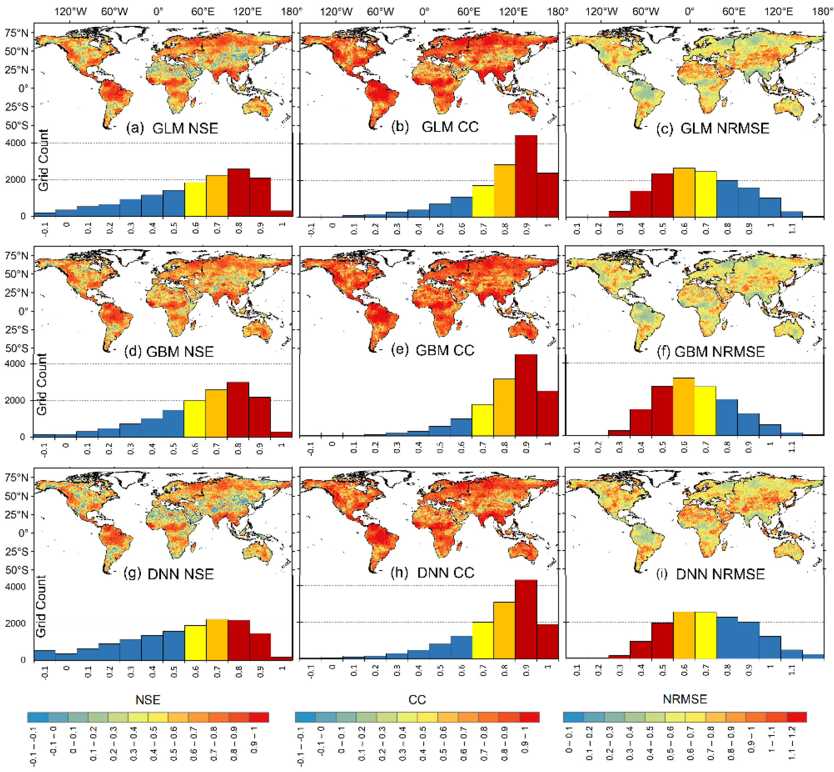
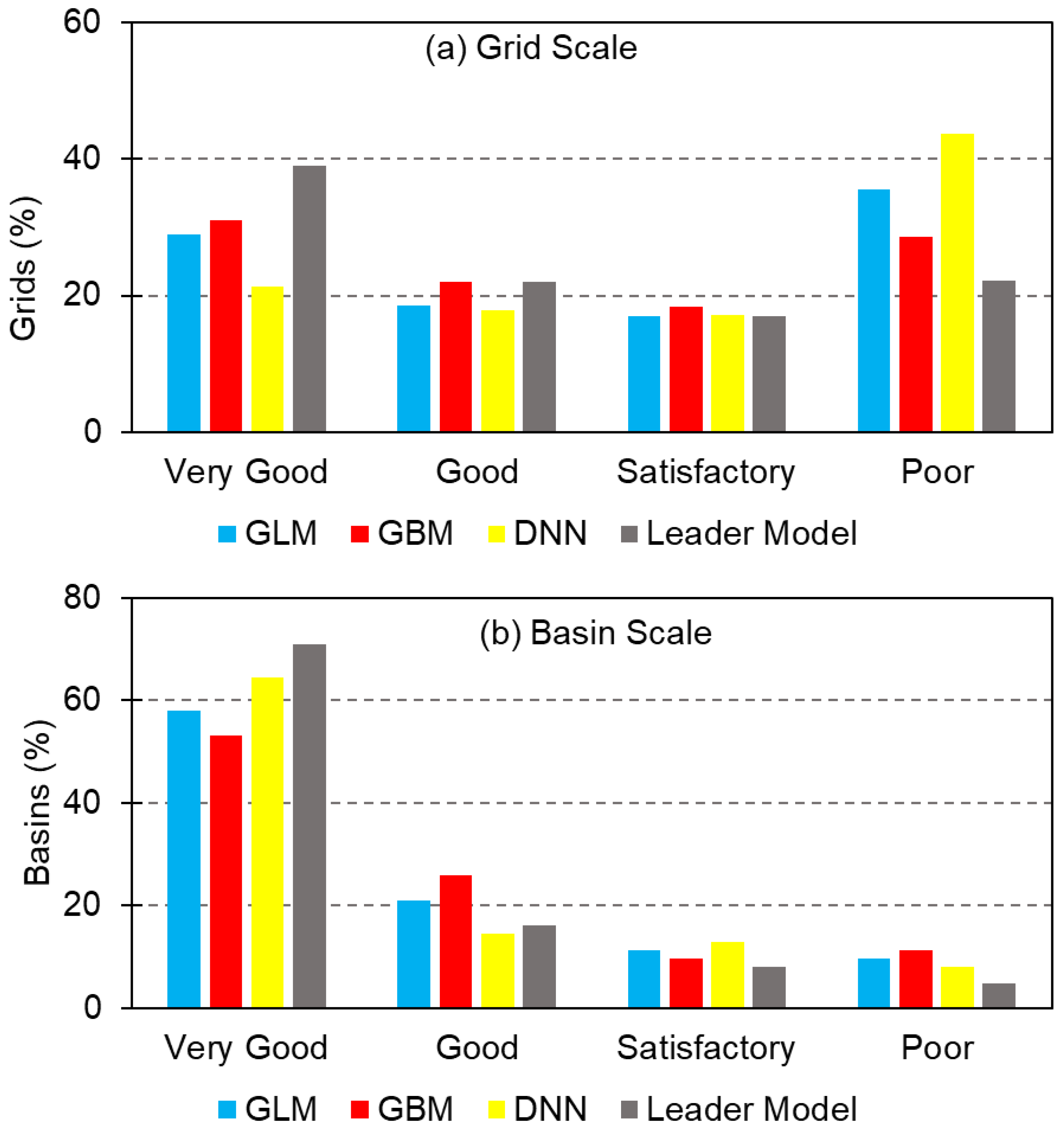
Figure 2. Flowchart showing model types, input data, and model structure used in this study.
Remotesensing 14 01565 g002
Figure 3. Spatial (maps) and frequency (bar plots) distributions of the grid-scale testing performance for the (ac) GLMs, (df) GBM models, and (gi) DNN models. The color-coded frequency distribution shows the very good (red), good (orange), satisfactory (yellow), and poor (blue) performance categories.
Remotesensing 14 01565 g003
Figure 4. Frequency distribution of (a) grid-scale and (b) basin-scale testing performance for the GLMs, GBM models, DNN models, and leader models.
Remotesensing 14 01565 g004
Figure 5. Spatial (left) and frequency (right) distribution of the grid-scale variable importance for (a) GLMs, (b) GBM models, and (c) DNN models.
Remotesensing 14 01565 g005
Figure 6. Spatial (left) and frequency (right) distributions of the grid-scale leader model (a) types, (b) testing NSE, (c) testing CC, (d), testing NRMSE, and (e) variable importance. The color-coded frequency distribution shows the very good (red), good (orange), satisfactory (yellow), and poor (blue) performance categories.
Remotesensing 14 01565 g006
Figure 7. Spatial and frequency (bar plot) distribution of the basin-scale testing performance for the (ac) GLM, (df) GBM, and (gi) DNN models. The color-coded frequency distribution shows the very good (red), good (orange), satisfactory (yellow), and poor (blue) performance categories.
Remotesensing 14 01565 g007
Figure 8. Spatial (left) and frequency (right) distribution of the basin-scale variable importance for (a) GLM, (b) GBM, and (c) DNN models.
Remotesensing 14 01565 g008
Figure 9. Spatial (left) and frequency (right) distribution of the basin-scale leader model (a) types, (b) testing NSE, (c) testing CC, (d), testing NRMSE, and (e) variable importance. The color-coded frequency distribution shows the very good (red), good (orange), satisfactory (yellow), and poor (blue) performance categories.
Remotesensing 14 01565 g009
Figure 10. Reconstructed TWSGRACE results for eight representative basins: (a) Niger, (b) Lake Chad, (c) Amazon, (d) Orinoco, (e) Flinders, (f) Murray, (g) Irrawaddy, and (h) Krishna. The actual TWSGRACE, reconstructed TWSGRACE, TWSGLDAS, and Humphrey and Gudmundsson (2019)-derived TWS (TWSHumphrey) time series are indicated by black dots, pink line, blue line, and green lines, respectively. The root-mean-square error for the testing set is plotted as error bar (pink shading) for the reconstructed TWSGRACE. The vertical yellow rectangle shows the gap period between the GRACE and GRACE-FO missions. The NSE between the actual TWSGRACE and reconstructed TWSGRACE, the actual TWSGRACE and TWSGLDAS, and actual TWSGRACE and TWSHumphrey are shown at the bottom of each subplot in pink, blue, and green text, respectively.
Remotesensing 14 01565 g010
Figure 11. Global monthly (August 2017–May 2018; (ak)) grid-scale reconstructed TWSGRACE data for the gap period between GRACE and GRACE-FO missions. The circles depict the regions where the reconstructed TWSGRACE captures the strong seasonal variations and extreme events [i.e., August–September high (red), April–May low (purple), April–May high (black), and October–November low (pink)]. The reconstructed TWSGRACE data over Australia for September 2017 (panel (l); top left corner) and September 2018 (panel (l); bottom left corner) are also shown. The United States’ extreme active hurricane season 2017 is compared with 2018 in Figure 11l (right panel).
Remotesensing 14 01565 g011
Table 2. The average testing performance matrices for grid and basin scales.
Grid Scale
GLMGBMDNNLeader Model
NSE0.55 ± 0.260.59 ± 0.230.49 ± 0.280.65 ± 0.20
CC0.74 ± 0.190.77 ± 0.150.73 ± 0.190.81 ± 0.13
NRMSE0.63 ± 0.190.61 ± 0.170.68 ± 0.190.56 ± 0.16
Basin Scale
GLMGBMDNNLeader Model
NSE0.74 ± 0.150.73 ± 0.170.75 ± 0.170.78 ± 0.14
CC0.87 ± 0.090.85 ± 0.110.88 ± 0.090.89 ± 0.07
NRMSE0.48 ± 0.150.49 ± 0.16 0.46 ± 0.16 0.43 ± 0.14
Table 3. Model testing performance comparison between this study and previous studies.
ReferenceRegion/BasinTheir Performance *This Study
Becker et al. [38]Amazon BasinCC = 0.9CC = 0.98
De Linage et al. [35]Amazon BasinR2 = 0.43NSE = 0.95
Long et al. [33]Southwest ChinaR2 = 0.57–0.91NSE = 0.84–0.95
Sośnica et al. [46]GlobalMean CC = 0.5Mean CC = 0.81
Zhang et al. [64]Yangtze BasinNSE = 0.83NSE = 0.84
Humphrey et al. [30]GlobalCC: Amazon = 0.96; Mississippi = 0.89; Volga = 0.90; Niger = 0.98CC: Amazon = 0.98; Mississippi = 0.9, Volga = 0.93
Niger = 0.91
Yang et al. [41]Northwest ChinaNSE = 0.2NSE = 0.52
Chen et al. [28]Northeast ChinaCC = 0.9CC = 0.66
Ahmed et al. [25]AfricaNSE = 0.54–0.94; CC = 0.79–0.97NSE = 0.65–0.93; CC 0.82–0.97
Hasan et al. [39]AfricaNSE = 0.72–0.94NSE = 0.65–0.93
Humphrey and Gudmundsson [66]GlobalMedian NSE < 0.5; CC < 0.75Median NSE = 0.69; CC = 0.85
Ferreira et al. [67]West AfricaCC = 0.88CC = 0.91
Sun et al. [68]IndiaCC = 0.94; NSE = 0.87CC = 0.84; NSE = 0.71
Li et al. [53]ChinaCC = 0.34–0.98; NSE = −0.21–0.95CC = 0.44–0.95; NSE = 0.76–0.98
Jing et al. [69]Nile River BasinCC = ~0.9CC = 0.91
Kenea et al. [31]EthiopiaR2 = 0.33–0.73; CC = 0.27–0.77NSE = 0.1–0.93; CC = 0.38–0.97
Li et al. [32]GlobalGrid CC = 0.63; Basin CC = 0.6Grid CC = 0.8; Basin CC = 0.89
Forootan et al. [48]GlobalCC = 0.89 (p = 0.00105)CC = 0.8; p < 0.00001
Sun et al. [71]GlobalBasin NSE = 0.7; CC = 0.9;
58% of grids @ NSE > 0.4
Basin NSE = 0.78; CC = 0.89; 87% of grids @ NSE > 0.4
Sun et al. [42]United StatesCC = 0.95; NSE = 0.85CC = 0.82; NSE = 0.67
Jing et al. [73]Pearl River BasinR2 = 0.56–0.71NSE = 0.81
Sohoulande et al. [72]United States41.2% of area @ R2 > 0.5 82.1% of area @ NSE > 0.5
Jeon et al. [74]GlobalNSE = 0.14–0.9NSE = 0.35–0.9
Yu et al. [75]CanadaCC = 0.96CC = 0.8
Tang et al. [76]Lancang-Mekong River basinBasin CC = 0.97; Grid CC = 0.9Basin CC = 0.98; Grid CC = 0.89
Yang et al. [77]AustraliaNSE = 0.96, CC = 0.98NSE = 0.66; CC = 0.81
Gyawali et al. [20]Texas Gulf CoastCC = 0.85, NSE = 0.73CC = 0.83; NSE = 0.67
Mo et al. [78]Global40 basins NSE = 0.44–0.9662 basins NSE = 0.44–0.97
* CC: correlation coefficient, NSE: Nash–Sutcliffe efficiency coefficient, R2: coefficient of determination, p: p-value.
Publisher’s Note: MDPI stays neutral with regard to jurisdictional claims in published maps and institutional affiliations.

