Modelling Within-Season Variation in Light Use Efficiency Enhances Productivity Estimates for Cropland

Abstract

Gross Primary Productivity (GPP) for cropland is often estimated using a fixed value for maximum light use efficiency (LUE_max) which is reduced to light use efficiency (LUE) by environmental stress scalars. This may not reflect variation in LUE within a crop season, and environmental stress scalars developed for ecosystem scale modelling may not apply linearly to croplands. We predicted LUE on several vegetation indices, crop type, and agroclimatic predictors using supervised random forest regression with training data from flux towers. Using a fixed LUE_max and environmental stress scalars produced an overestimation of GPP with a root mean square error (RMSE) of 6.26 gC/m²/day, while using predicted LUE from random forest regression produced RMSEs of 0.099 and 0.404 gC/m²/day for models with and without crop type as a predictor, respectively. Prediction uncertainty was greater for the model without crop type. These results show that LUE varies between crop type, is dynamic within a crop season, and LUE models that reflect this are able to produce much more accurate estimates of GPP over cropland than using fixed LUE_max with stress scalars. Therefore, we suggest a paradigm shift from setting the LUE variable in cropland productivity models based on environmental stress to focusing more on the variation of LUE within a crop season.

1. Introduction

Gross Primary Productivity (GPP) and Net Primary Productivity (NPP) underpin many global estimates of crop production with remote sensing. They express the rate of carbon fixation by plants, from which measures such as cumulative biomass production and yield can be derived. For example, several global crop yield maps are now available which estimate grain yield from GPP or NPP [1,2]. Furthermore, there is increasing use of remote sensing methods to monitor carbon dynamics over agricultural lands [3,4]. Therefore, it is important that the accuracy of productivity estimation methods is continually monitored and improved.

Remote sensing estimates of productivity at a point in time are generally based on a Production Efficiency Model since Monteith [5,6] defined productivity as a function of incoming solar radiation and light use efficiency (LUE) (Equation (1)):

$$GPP=fPAR\times PAR\times LUE,$$

(1)

where $GPP$ is a function of photosynthetically active radiation ($PAR$), the fraction of this which is absorbed by plants ($fPAR$), and $LUE$. This can be applied to either $GPP$ or NPP, and $LUE$ values may refer to either measure [7,8,9,10]. We focus on GPP in this paper as it forms the basis of several current cropland products [1,11,12,13].

Early efforts to optimise Production Efficiency Model parameters focused on fPAR, and attention has now turned to the LUE parameter, which has been recognised as a critical component of the error budget in remote sensing GPP models [14,15,16]. Various approaches to setting the LUE parameter exist, which include assuming a globally fixed value, assuming a fixed value for each functional type of vegetation (C3 grass, C4 grass, and trees), or varying LUE dynamically with vegetation type and environmental stressors [8,14]. The latter approach, known as the Carnegie–Ames–Stanford Approach (CASA) has been widely applied to both NPP and GPP estimation for field crops [17,18] (Equation (2)):

$$GP{P}_{\mathrm{CASE}}=fPAR\times PAR\times LU{E}_{\max }\times TS\times VS\times SMS,$$

(2)

where maximum LUE ($LU{E}_{\max }$) is reduced below its potential by temperature stress ($TS$), vapor stress ($VS$), and soil moisture stress ($SMS$) scalars to give LUE_CASA. This is a simple yet effective means of capturing environmental variation in LUE [8]. Alternatively, Donohue et al. [14] varied LUE based on the proportion of diffuse radiation which met or outperformed the stress scalar approach for accurate GPP estimation at a continental scale. However, each method relies on an accurate starting value for $LU{E}_{\max }$. Lobell et al. [8] recognised that LUE, and thereby LUE_max, could be predicted based on relationships with satellite-derived vegetation indices [19,20]. For example, canopy greenness, as a proxy for crop maturity and stress, such as nutrient deficiency, may be useful predictors of LUE [21,22]. We sought to combine vegetation indices with crop type and agroclimatic information to test whether a machine learning method could accurately predict cropland LUE.

A contrasting approach for setting LUE for agricultural applications is setting a fixed LUE_max based on information such as crop type, and sometimes soil fertility and fertiliser regimes [8]. For example, the Global Yield Mapper in Google Earth Engine (GYMEE) notes uncertainty in defining LUE_max for crop type and applies 2.5 gC/MJ/day for C3 crops and 3.5 gC/MJ/day for C4 crops [1]. Similarly, the Python implementation for the Surface Energy Balance Algorithm (PySEBAL) documentation for estimating crop biomass production and evapotranspiration recommends LUE_max values of 2.5 gC/MJ/day and 4.5 gC/MJ/day for C3 and C4 crops, respectively [12,13,23].

However, fixed LUE_max measured at the field or plant levels may be much greater than LUE_max applicable to remote sensing scales. Calculating in situ LUE_max from flux tower GPP measurements has revealed overestimation of LUE_max for croplands and therefore overestimation of remotely sensed GPP. For example, Wang et al. [9] calculated LUE_max values ranging from approximately 2.3 to 3.7 gC/MJ/day for maize and 1.4 gC/MJ/day for wheat from flux tower sites. Similarly, Xin et al. [24] calculated mean values of 2.78 and 1.64 gC/MJ/day for maize and soybean, respectively. These values are generally greater than estimates of LUE_max for global or continental products such as the Moderate-Resolution Imaging Spectroradiometer (MODIS) GPP, but less than values generated in field experiments. This has led to an underestimation of cropland GPP in continental products and overestimation of GPP when fixed LUE_max values are used in cropland-specific applications [7,24,25].

In addition to overestimation of LUE_max, there are two main reasons why CASA with fixed LUE_max may not adequately quantify LUE for cropland. The first is that neither a fixed coefficient for LUE_max nor the stress scalars (Equation (2)) account for within-season variation in LUE, which has been demonstrated for a range of field crops. For example, Gitelson and Gamon [15] show that LUE varied within maize- and soybean-growing seasons, both before (LUE_inc) and after (LUE_total, referred to as LUE in this paper) fPAR was accounted for, and Lecoeur and Ney [26] show a similar temporal pattern for field peas. Gitelson et al. [16] recognised the two to three-fold variation in LUE within growing seasons for maize and soybean meant this source of variation “should be accounted for in LUE models”.

The second reason that CASA may not apply well to croplands is that stress scalars may be less relevant in managed environments, especially irrigated croplands, than in other vegetated land types. Lobell et al. [8] found that omitting stress scalars from CASA (Equation (2), adapted for NPP) improved NPP estimation accuracy for irrigated and temperature-resistant crops. Therefore, an alternative approach to setting the LUE variable for cropland productivity estimations based primarily on within-season variation in crop growth may be superior to the CASA method.

In this paper, we investigate whether a non-parametric, machine learning, predictive model for LUE based on satellite-derived vegetation indices and agroclimatic variables can give more accurate GPP predictions for cropland than CASA. This approach differs from previous studies in its non-parametric approach, and specificity and scalability to croplands. Relationships between vegetation indices and both LUE and GPP for cropland have been investigated by Peng et al. [27], and Peng and Gitelson [28], though these have generally focused on parametric modelling approaches relating GPP or LUE to individual indices. Non-parametric random forest approaches have been applied to prediction of LUE at the global scale by Wei et al. [29] based predominantly on meteorological and land use/land cover predictors. Our approach is unique in its use of both agroclimatic and vegetation indices as predictor variables that have previously been investigated separately, its specificity to cropland and crop type, and its scalability due to reliance on globally-available Landsat and climate data.

To this end, flux tower data were used to derive GPP_{in situ} and LUE_{in situ}, and demonstrate how these varied within a crop season and between crop type. The in situ values were compared with satellite-based estimates of LUE_CASA, and GPP_CASA. LUE_{in situ} was also used to train a machine learning model with satellite data, crop type, and agroclimatic variables as predictors. The importance and dependence of each predictor in the model were evaluated to assess which variables best predicted LUE, and to understand how vegetation indices and agroclimatic information relate to LUE within a crop season. Finally, the accuracy of GPP_CASA estimates was compared with the accuracy of predicted GPP ($G\widehat{P}P$) using predicted LUE ($L\widehat{U}E$_RF) from the random forest regression model.

2. Materials and Methods

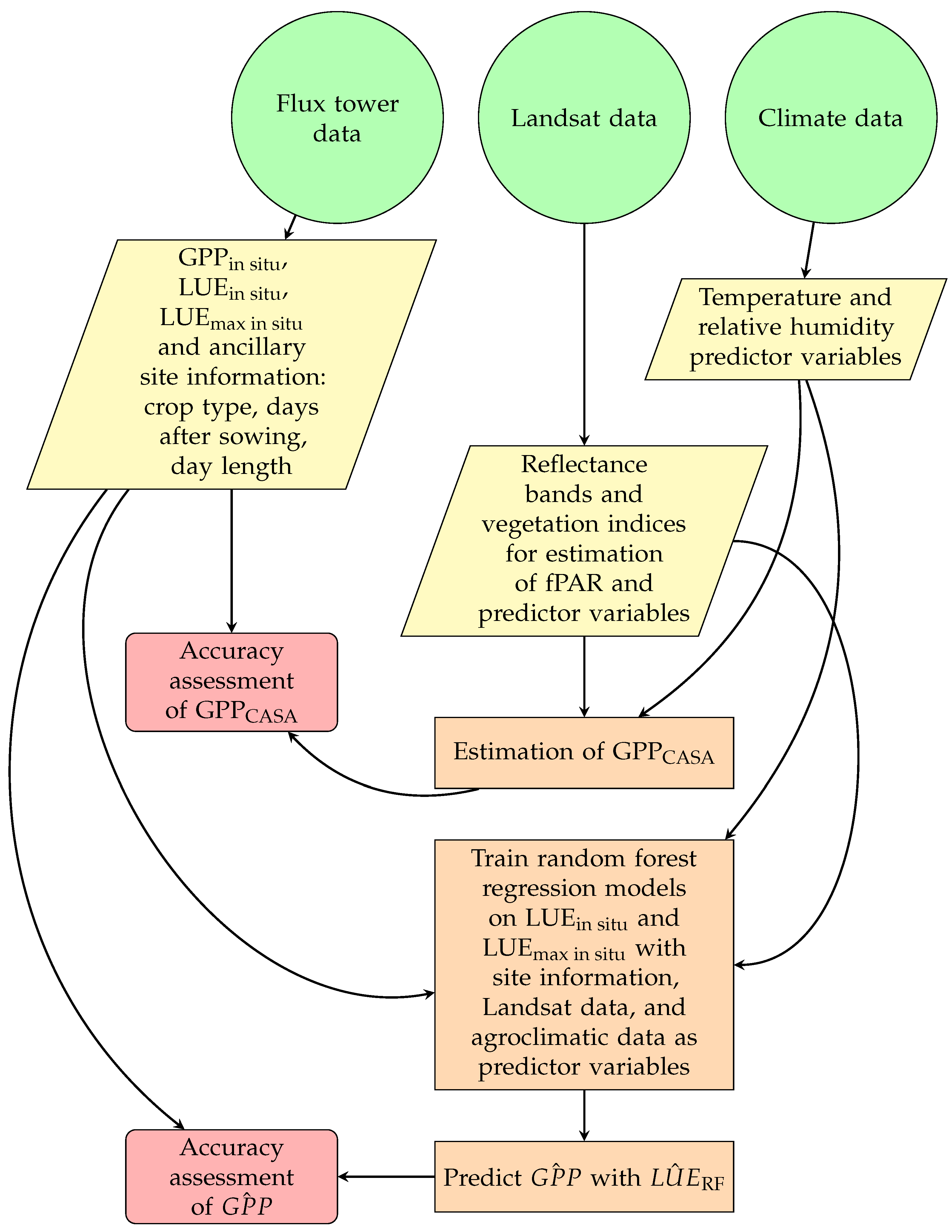
2.1. Overview of Methodology

We used flux tower data for GPP_{in situ} to assess the accuracy of remotely sensed GPP. From this, LUE_{in situ} was also derived, which was then used as training data for the predictive model. This process is summarised in Figure 1 and details of LUE_{in situ} and LUE_{max in situ} estimation are provided in the following sections.

2.2. Flux Tower Data

Flux tower sites corresponding to cropland were identified within the FLUXNET database [30]. From these, sites with known crop species were selected so accuracy could be assessed between crop functional type (C3 and C4) and crop species.

Table 1. Flux tower sites used to derive GPP_{in situ} and LUE_{in situ}.

Site Name	Site Code	Years Active	Crop Species	Observations
Cheorwon Rice paddy	KR-CRK [31]	2015–2018	Rice	15
Philippines Rice Institute flooded	PH-RiF [32]	2012–2014	Rice	19
Humnoke Farm Rice Field A	US-HRA [33]	2017	Rice	4
Humnoke Farm Rice Field C	US-HRC [34]	2017	Rice	4
Mead-irrigated continuous maize site	US-Ne1 [35]	2001–2013	Maize	47
Mead-irrigated maize–soybean rotation site	US-Ne2 [36]	2001–2013	Maize (odd years), soybean (even years)	33
Mead-rainfed maize–soybean rotation site	US-Ne3 [37]	2001–2013	Maize (odd years), soybean (even years)	46

shows the FLUXNET tower sites used. Data were downloaded from the FLUXNET database in daily format. The number of observations was determined by the number of days during active years where a clear Landsat 7 or 8 image was available over the site, and crop growth was occurring, which was defined as GPP being ≥0.1 gC/m².

2.3. Satellite and Climate Data

At present, Landsat mission satellites offer useful spatial resolution and historical temporal coverage for cropland applications. Several software applications readily support GPP calculations from Landsat images. We used the Python script PySEBAL because it produces a biomass estimate based on GPP from the CASA equation, and also gives outputs required to calculate stress scalars, such as transpiration and evaporation [12,23].

Both Landsat-7 and Landsat-8 imagery were used to cover the epoch from 2001 to 2018 (Table 1). Collection 1 Level-1 images with less than 20% cloud cover were downloaded from the USGS Earth Explorer website. Landsat band digital numbers were converted to top of atmosphere reflectance values using the scaling coefficients in metadata files. Landsat-7 imagery must be spatially gapfilled to correct the scan line corrector (SLC) failure. Jaafar et al. [38] reported more consistent outputs from PySEBAL when Landsat-7 bands were gapfilled using the ‘focal’ function from the R package ‘raster’ [39]. Therefore, a $3\times 3$ moving window was applied to Landsat-7 bands using the ‘focal’ function to fill pixels identified as having null values in R version 4.1.1 [40].

PySEBAL requires 24 average and instantaneous shortwave radiation, wind speed, air temperature, air pressure and relative humidity as inputs. These were derived from the National Aeronautics and Space Administration’s Global Land data assimilation system (GLDAS) [41]. Climate observations closest in time to the Landsat overpass time were used as the instantaneous values while means were calculated across the eight observations for each day to form 24 h average values [11,12].

To complete the required inputs for PySEBAL, a digital elevation model (DEM) was acquired from the Shuttle Radar Topography Mission (SRTM) [42] and soil physical properties were derived from the HiHydroSoil dataset [43].

2.4. Remote Sensing Estimation of Gross Primary Productivity and Light Use Effiency

2.4.1. Analysis Boundary

All remotely sensed measures were masked to an approximate cropland ecosystem boundary which was defined as a $10\times 10$ matrix of Landsat pixels surrounding the flux tower, giving an area of approximately 300 m × 300 m. This area was chosen across sites because flux tower height was generally set at a level which best captured the immediate field and eliminated surrounding landscapes [44], and this area generally fell within the target fields while enabling consistent spatial sampling from each site. This area was also consistent with former studies on flux tower sites which have used both Landsat and MODIS resolutions and therefore enhanced comparability of error across approaches [22,24,27,45]. The mean of values across the 10 × 10 matrix were taken for all remotely sensed variables to generate the final dataset with the number of observations shown in Table 1.

More recent flux tower initiatives have captured meteorological variables which enable calculation of flux footprints for use in future studies [46,47].

2.4.2. Remotely Sensed Gross Primary Productivity

Initial estimates of GPP_CASA were used to calculate a baseline error against GPP_{in situ}; this is the foremost accuracy assessment in Figure 1. The output map of biomass production from PySEBAL expresses GPP in kg/ha/day as calculated in Equation (2) [11,12,23]. PySEBAL was run with the recommended LUE_max values of 2.5 gC/MJ/day for C3 crops (rice, soy) and 4.5 gC/MJ/day for C4 crops (maize). This output map was multiplied by 0.1 to convert from kg/ha to gC/m².

2.4.3. Calculation of Light Use Efficiency and Stress Scalars

LUE_{in situ} and LUE_{max in situ} corresponding to Landsat overpass dates were calculated by inversion of the GPP (Equation (1)) and CASA equations (Equation (2)) [8,10]. Daily GPP_{in situ} and incoming shortwave radiation were available from FLUXNET datasets for each site. Other parameters were kept consistent with the PySEBAL script [12,23] due to its specificity to cropland and its similarity to other GPP estimates for cropland including GYMEE [1]. The variable, fPAR, was calculated on Landsat images as:

$$fPAR=-0.161+1.257\times NDVI,$$

(3)

conditional on the Normalised Difference Vegetation Index ($NDVI$) being ≥0.125, below which $fPAR$ was set as 0. This definition of $fPAR$ has been widely applied to cropland applications since Bastiaannssen and Ali [48] aggregated coefficient and intercept values from several cropland experiments, including the work of Daughtry et al. [49] on maize and soybean.

$PAR$ was calculated as:

$$PAR=Rs\times 0.48\times 0.0864,$$

(4)

where $PAR$ is 48% of incoming shortwave radiation ($Rs$) [48] and 0.0864 converts W/m² to MJ/m²/day.

Temperature stress ($TS$) was calculated based on Stewart [50,51] and Jarvis [52] as:

$$TS=\frac{(T-T_l)\times {(T_h-T)}^{J}c}{(K_t-T_l)\times {(T_h-K_t)}^{J}c}$$

(5)

where T is the average daily temperature and $Jc$ is the Jarvis coefficient, calculated as:

$$Jc=\frac{T_h-K_t}{K_t-T_l},$$

(6)

where $Th$, $Kt$, and $Tl$ are the upper limit, optimum value, and lower limit of temperatures (${}^{\circ }$C) for stomatal conductance, respectively. These constants were made consistent with the PySEBAL script [12,23] Constants used in Equations (5) and (6) are presented in

Table 2. Constant values used for calculation of temperature stress in the estimation of GPP_CASA.

Constant	Definition	Source
$Tl$	0 ${}^{\circ }$C	[53,54]
$Kt$	23 ${}^{\circ }$C	[53,54]
$Th$	35 ${}^{\circ }$C	[53,54]

.

Vapor stress ($VS$) was calculated based on Oren et al. [55], and Fuchs and Stanghellini [56], as:

$$VS=0.88-0.183\times log(E_{sat}-E_{act}),$$

(7)

where $E_{sat}$ and $E_{act}$ are the saturated and actual vapor pressure (kPa), respectively.

Soil moisture stress ($SMS$) was calculated as the ratio of actual ($T_{act}$) to potential ($T_{pot}$) 24 h transpiration [57]:

$$SMS=T_{act}/T_{pot},$$

(8)

where $T_{act}$ and $T_{pot}$ were taken from PySEBAL output maps and masked according to Section 2.4.1.

2.5. Modelling Light Use Efficiency

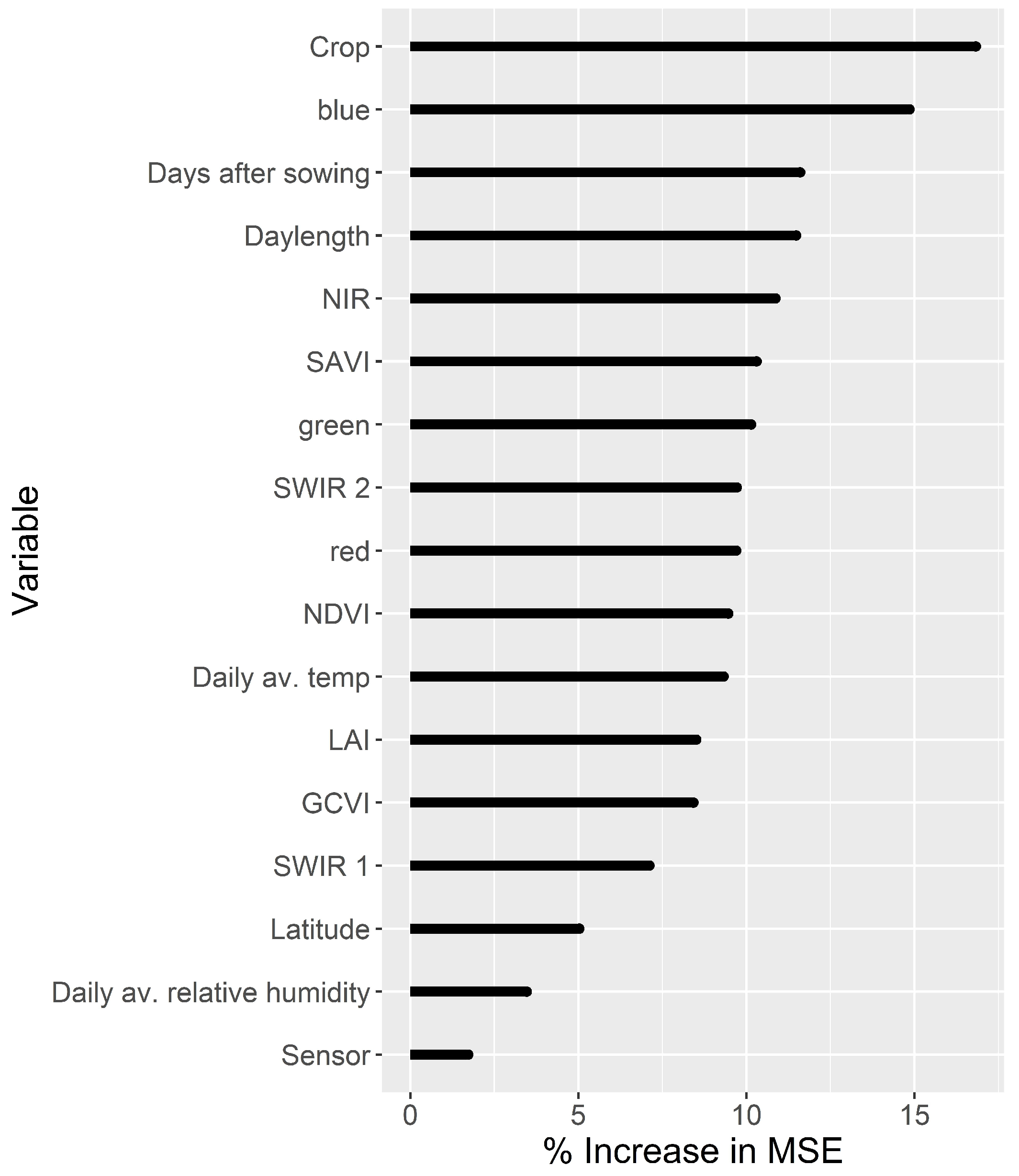
2.5.1. Predictor Variables

Several satellite bands, vegetation indices, and agroclimatic variables were used as predictors for LUE. Although vegetation indices vary with crop maturity [16], we included both days after sowing (DAS) and day length as predictor variables to capture potential within-season variation in LUE. Using DAS as a predictor overcame the limitation of using day of year which may be site, rather than crop type, specific. The inclusion of these predictors also enabled the relative importance of seasonality and vegetation indices to be investigated.

Satellite-derived data were masked according to the analysis boundary as per Section 2.4.1. The details of each predictor variable used in the random forest regression models are summarised in

Table 3. Definition of predictor variables used to train predictive models for light use efficiency.

Group	Variable	Definition	Source
Satellite bands	Blue	Landsat-7: 0.45–0.52 $\mathsf{\mu }$m Landsat-8 0.45–0.51 $\mathsf{\mu }$m	[58]
	Green	Landsat-7: 0.52–0.60 $\mathsf{\mu }$m Landsat-8 0.53–0.59 $\mathsf{\mu }$m	[58]
	Red	Landsat-7: 0.63–0.69 $\mathsf{\mu }$m Landsat-8 0.64–0.67 $\mathsf{\mu }$m	[58]
	Near Infrared (NIR)	Landsat-7: 0.77–0.90$\mathsf{\mu }$m Landsat-8 0.85–0.88 $\mathsf{\mu }$m	[58]
	Shortwave Infrared 1 (SWIR 1)	Landsat-7: 1.55–1.75 $\mathsf{\mu }$m Landsat-8 1.57–1.65 $\mathsf{\mu }$m	[58]
	Shortwave Infrared 2 (SWIR 2)	Landsat-7: 2.09–2.35 $\mathsf{\mu }$m Landsat-8 2.11–2.29 $\mathsf{\mu }$m	[58]
Vegetation indices	Normalised Difference Vegetation Index (NDVI)	$\frac{(NIR-Red)}{(NIR+Red)}$	[59]
	Green Chlorophyll Vegetation Index (GCVI)	$\frac{NIR}{Green}-1$	[60]
	Leaf Area Index (LAI)	From PySEBAL	[12,23]
	Soil-Adjusted Vegetation Index (SAVI)	$1.5\times \frac{(NIR-Red)}{(NIR+Red+0.5)}$	[61]
Site and image information	Crop Type		Table 1
	Sensor	Landsat-7 or Landsat-8
	Latitude		Table 1 [30]
	Day length	Calculated on latitude and DOY using geosphere R package	[62]
Agroclimatic variables	Daily Average Temperature		Section 2.3
	Daily Average Relative Humidity		Section 2.3
	Days after Sowing (DAS)	Approximate sowing dates taken from regional crop calendars	[63,64,65]

.

2.5.2. Random Forest for Light Use Efficiency

Random forests [66] is a machine learning algorithm which was used to develop a predictive model for LUE using the randomForest package in R [67]. The method uses an ensemble approach to build a large number of regression trees on bootstrap samples (typically 500) of the original dataset with varying inputs. Predictions from regression trees are aggregated to estimate ${L\widehat{U}E}_{\mathrm{RF}}$ and uncertainties can be quantified through the assessment of quantiles from the bootstrap distribution of outputs.

Three predictive models for LUE were trained and evaluated: one trained on LUE_{in situ} with all 17 variables in Table 3 and one without crop type, as this may not always be known to users. A third model was also trained on LUE_{max in situ} using all 17 predictors to determine whether this parameter could be accurately modelled. Variable importance was extracted from the model and expressed as the percentage increase in mean squared error (MSE). The out-of-bag (OOB) predictions for $L\widehat{U}E$_RF were used to calculate GPP using Equation (1). We refer to this as $G\widehat{P}P$. An OOB prediction for an observation, LUE_i, is based on trees which do not use the in situ value of LUE_i in the bootstrapped training sample. Evaluations based on OOB predictions are therefore not prone to overfitting and are an alternative to traditional cross validation. The accuracy of $G\widehat{P}P$ against GPP_{in situ} was evaluated using the root mean square error (RMSE) and mean error (ME). These formed the latter accuracy assessment shown in Figure 1, which was compared with the accuracy for GPP_CASA (Equation (2)), the foremost accuracy assessment in Figure 1. Prediction uncertainty was calculated for each random forest model. This was presented as the standard error on the OOB prediction and calculated using the randomForestCI package [68].

3. Results

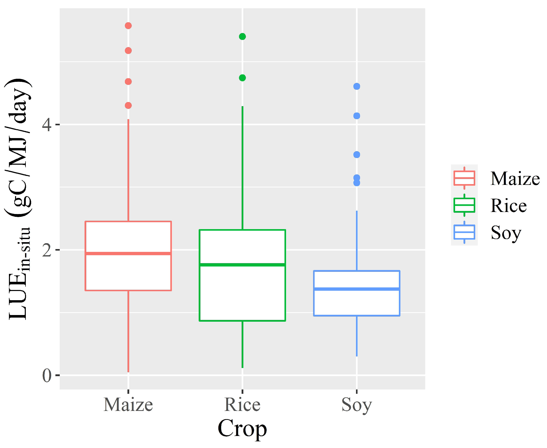
3.1. In Situ Light Use Efficiency

LUE_{in situ} was mostly distributed between 1 and 4 gC/MJ/day (Figure 2). Maize gave the highest median, and each median was below 2 gC/MJ/day.

The temporal pattern of LUE_{in situ} generally reflected the pattern in GPP_{in situ}. Both GPP_{in situ} and LUE_{in situ} rose to reach a mid-season maximum before declining, with the rate and timing of increase and decline varying between crop type (Figure 3). However, the pattern in GPP_{in situ} initially increased at an increasing rate, showing a sigmoidal plant growth curve, while LUE_{in situ} tended to show a more constant rate of increase. This was particularly evident in the locally fitted polynomial curves for soybean (Figure 3).

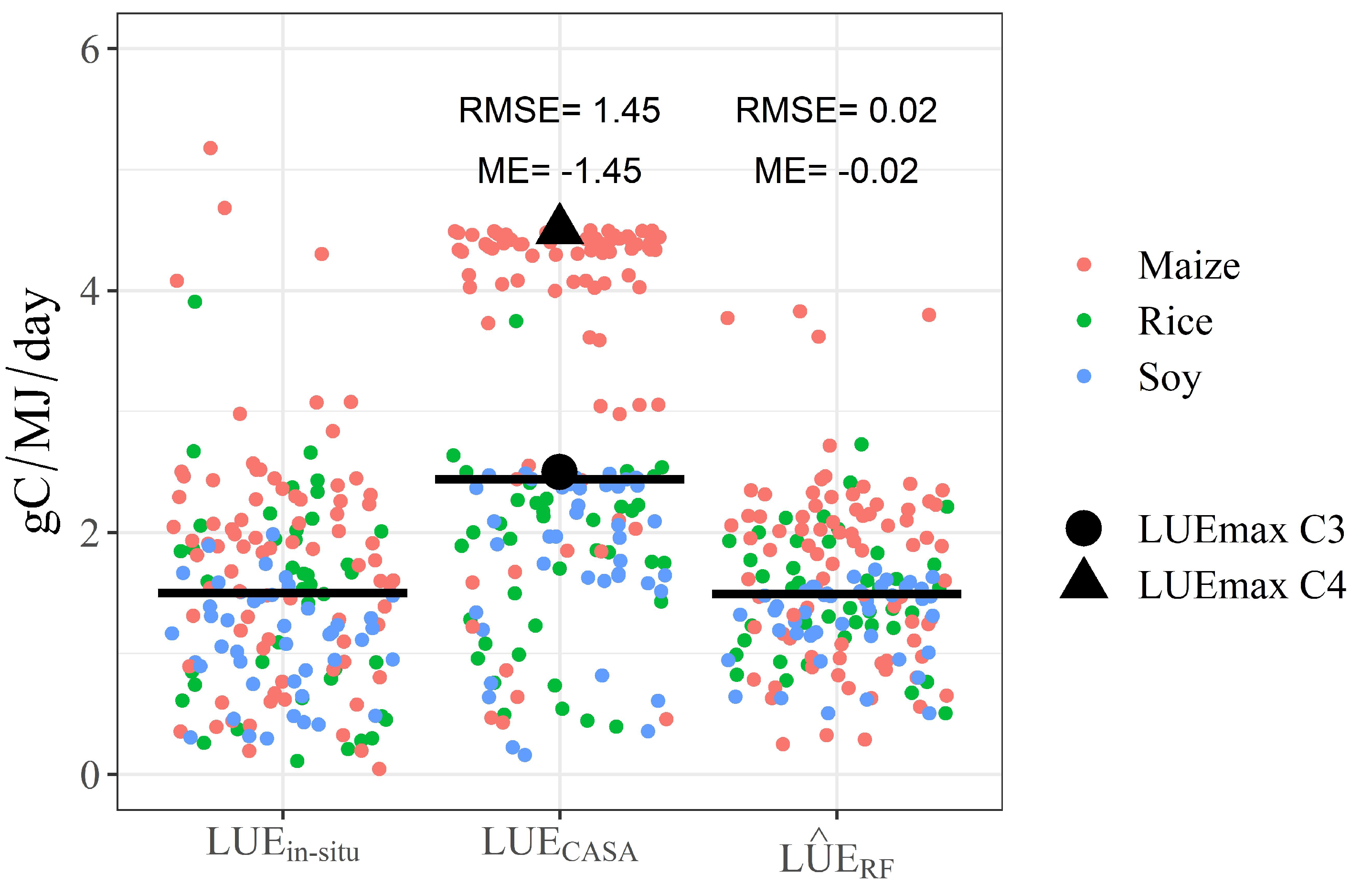
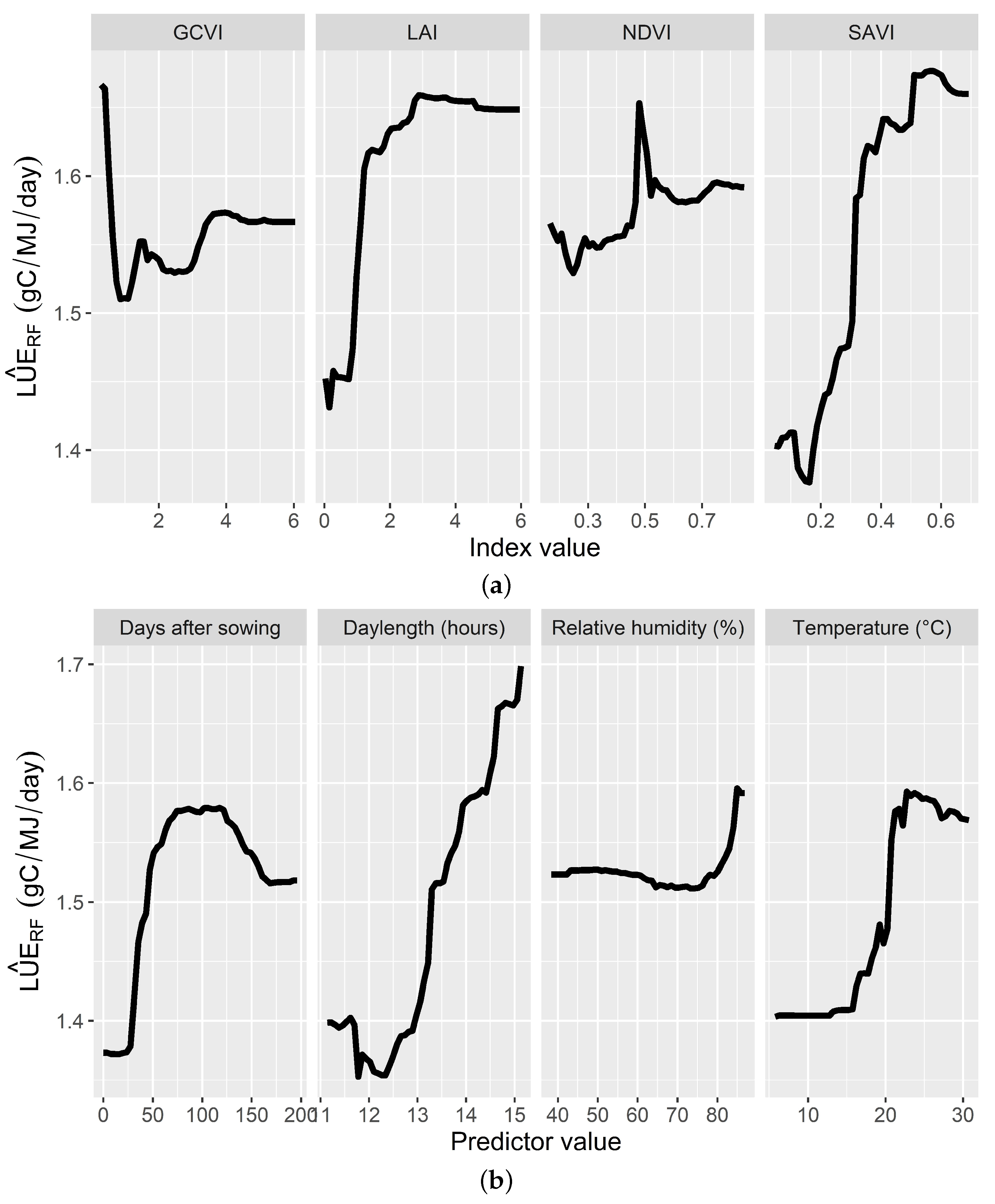
3.2. Prediction of Light Use Efficiency

The model which included crop type produced a higher $R^2$ and lower mean of squared residuals (

Table 4. Performance of random forest prediction models for light use efficiency (LUE) (Models 1 and 2) and LUE_max (Model 3) expressed as percentage of variation in LUE_{in situ} or LUE_{max in situ} explained by variation in out-of-bag predictions (R${}^2$) for LUE/LUE_max and mean of squared residuals.

Measure	Model 1: All Predictors in Table 3	Model 2: No Crop Type Predictor	Model 3: All Predictors in Table 3, LUEmax as Response
R${}^2$	62.94%	58.30%	14.19%
Mean of squared residuals	0.28	0.32	0.87

), indicating that crop type is an important predictor of LUE. This was reflected in the variable importance results (Figure 4). However, the OOB predictions for LUE_max from random forest models did not explain much variation in LUE_{max in situ} (Table 4). Additionally, Figure 5 shows that the stress scalars in the CASA Equation (2) do not sufficiently downscale the fixed LUE_max values to match LUE_{in situ}, especially for maize. The negative mean error indicates that LUE_CASA is an overestimate of LUE_{in situ}. ${L\widehat{U}E}_{\mathrm{RF}}$ from Model 1 (Table 4) shows a much closer distribution to that of LUE_{in situ}. For this reason, only Models 1 and 2, which give ${L\widehat{U}E}_{\mathrm{RF}}$, not LUE_max, were chosen for further evaluation.

Crop type was the most important predictor in Model 1 (Figure 5), reflecting variation in LUE_{in situ} between crops shown in Figure 2. Thereafter, the agroclimatic variables—day length, DAS, and temperature—were relatively important predictors. Vegetation indices were of similar importance. Satellite bands were scattered amongst other predictors in terms of importance, and relative humidity was relatively unimportant.

Partial dependence plots (Figure 6) from random forest Model 1 show that LAI values less than approximately 2 reduced ${L\widehat{U}E}_{\mathrm{RF}}$. Higher SAVI and NDVI were associated with greater ${L\widehat{U}E}_{\mathrm{RF}}$, while GCVI between approximately −0.5 and 1 reduced predicted values. Partial dependence on DAS reflected temporal patterns in GPP and LUE shown in Figure 3. Greater day length was associated with higher ${L\widehat{U}E}_{\mathrm{RF}}$, as was average temperature, although values greater than approximately 25 ${}^{\circ }$C reduced predictions.

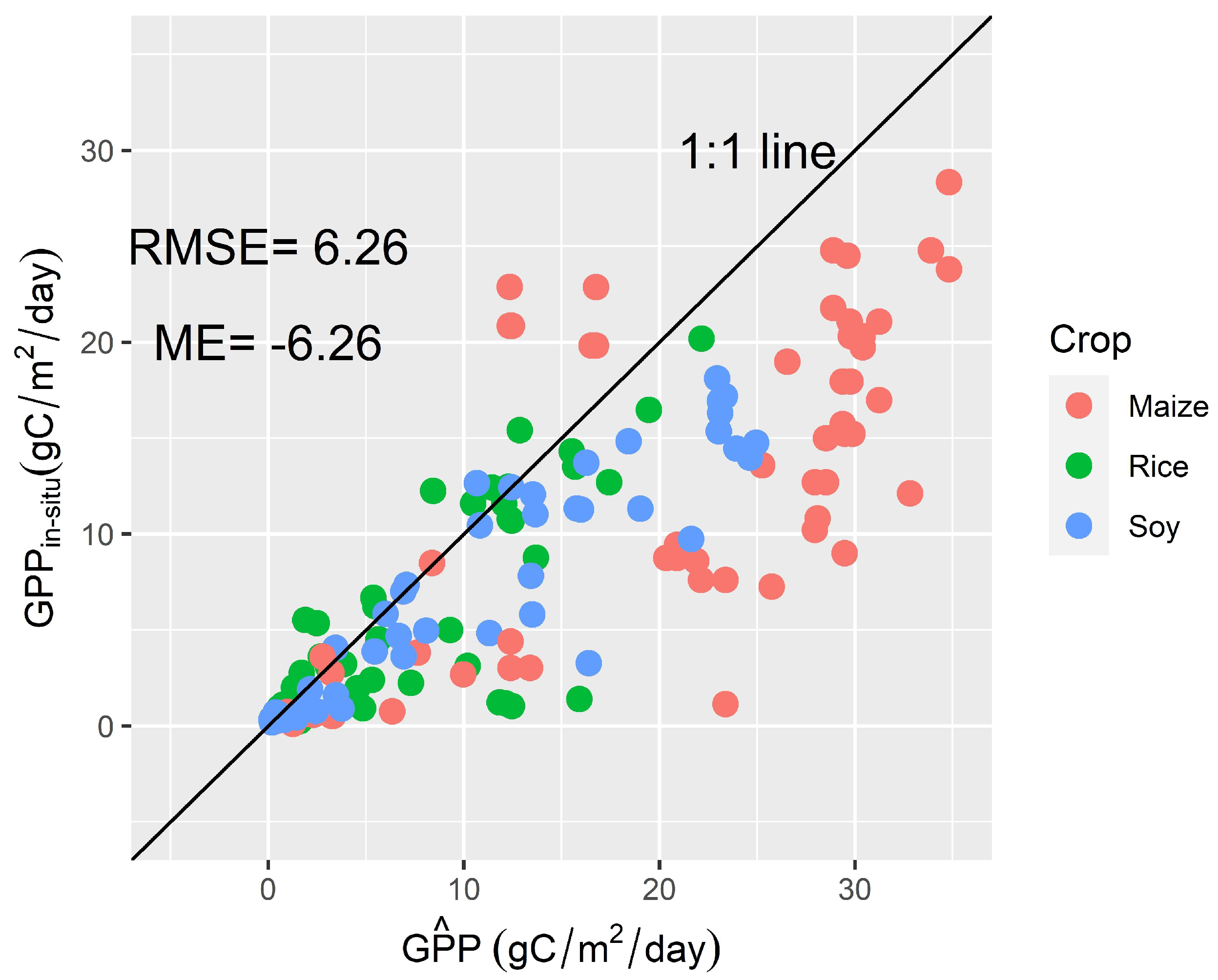
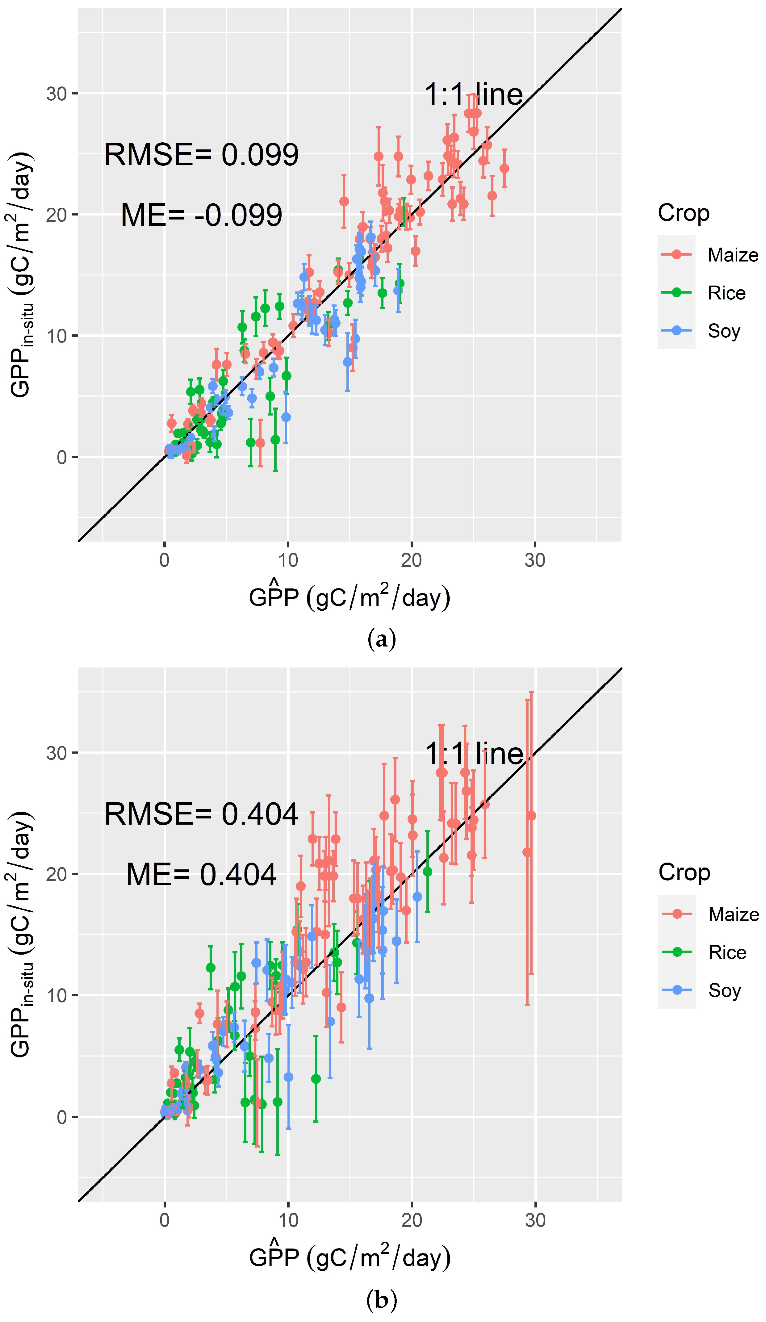
3.3. Estimation of Gross Primary Productivity

CASA led to overestimation of GPP, as indicated by the negative ME, especially for maize (Figure 7). Estimating GPP with ${L\widehat{U}E}_{\mathrm{RF}}$ improved accuracy and reduced the RMSE between GPP_{in situ} and $G\widehat{P}P$ (Figure 8). Prediction uncertainty was greater and estimate accuracy was lower in the model that did not include crop type as a predictor (Figure 8).

4. Discussion

${L\widehat{U}E}_{\mathrm{RF}}$ from a machine learning model produced more accurate estimates of $G\widehat{P}P$ than GPP_CASA estimated with a fixed LUE_max and stress scalars, as shown in Figure 8. This was because CASA gave grossly overestimated GPP estimates (Figure 7) due to overestimation of LUE_max and insufficient downscaling from the stress scalars (Figure 4). These findings are consistent with Cheng et al. [25] who, using some of the flux tower sites in Table 1, found that CASA overestimated GPP by a RMSE of approximately 6 gC/m²/day, while the MODIS MOD17 GPP product underestimated cropland GPP by a RMSE of approximately 12 gC/m²/day. This means that using crop-specific LUE_max values in CASA is likely to produce more accurate estimates of GPP than continental GPP products over cropland, and that accuracy can be further improved by varying LUE using a predictive model.

Furthermore, prediction of ${L\widehat{U}E}_{\mathrm{RF}}$ on a combination of agroclimatic and vegetation index predictors for calculation of $G\widehat{P}P$ gave more accurate estimates than other approaches applied to these flux tower sites. Peng and Gitelson [28,69] produced RMSEs of 2.75 and 2.9 gC/m²/day, respectively, by focusing on GCVI and NDVI as predictors. RMSEs between 1 and 2 gC/m²/day were achieved by incorporating other indices such as the LAI and Wide Dynamic Range Vegetation Index (WDRVI) [27,45]. Our estimation of RMSEs < 1 gC/m²/day (Figure 8), across similar ranges of GPP_{in situ}, for the same flux tower sites demonstrates the enhanced accuracy attributable to the machine learning approach encompassing within-season variation.

Our findings demonstrate that varying LUE dynamically over a cropping season will produce more accurate estimates of remotely sensed GPP. Figure 3 shows that LUE_{in situ} varies within seasons, and variables related to seasonality, namely DAS and day length, have been highlighted as important by the random forest model (Figure 5). This is also supported by the partial dependence patterns of the random forest model on DAS, NDVI, and day length (Figure 5 and Figure 6), which reflects patterns identified in Figure 3. Neither the LUE_max or stress scalars in CASA account for within-season variation in LUE. We suggest that this source of variation should be a primary component of productivity estimation methods for cropland.

Furthermore, Figure 4 shows that stress scalars did not sufficiently reduce LUE_max to reflect LUE_{in situ}, especially for maize. This may be because temperature, vapor, and soil moisture stress did not explain much variation in LUE_{in situ}, though setting LUE_max too high also contributed. A weak relationship between the stress scalars and LUE_{in situ} may also explain the poor predictive ability of Model 3 with LUE_max as the response (Table 4). This corresponds to Lobell et al. [8] who found greater NPP estimate accuracy with CASA when stress scalars were omitted for irrigated and temperature-resistant crops. They attributed this to the stress scalars being inappropriate indicators of variation in LUE for some croplands where stress may be overcome by either genotypic (temperature stress-resistant cultivars) or agronomic (irrigation) management. Additionally, components of CASA have been criticised for their weak relationship to LUE. Sinclar and Muchow [70] argued that the Occam’s Razor philosophy of preferring hypotheses with fewer assumptions should be applied to determining crop LUE in their criticism of relating vapor pressure deficit to LUE. They cited minimal statistical support for a meaningful relationship between these variables. This is supported by our finding that relative humidity was a relatively unimportant predictor of LUE (Figure 5).

Varying LUE within season is specific to remote sensing for croplands because crop maturity and type are generally uniform in space and time within fields, contrasting other land types with heterogeneous vegetation type and age [8]. We have demonstrated that approaches that vary crop LUE primarily on environmental stresses may lack relevance to croplands, and productivity modelling approaches should place more importance on within-season variation. Environmental stress-based approaches may remain applicable to ecological applications where a fixed LUE_max reflects a central value for heterogeneous vegetation and plant growth is more greatly influenced by temperature and soil moisture stress [14,17]. However, such approaches may also be enhanced by consideration of diffuse radiation [14,70].

The importance of crop type and predictors relating to within-season variation in the random forest model (Figure 5) show that these variables best reflect the photosynthetic properties of a crop at a given satellite overpass date. The better prediction accuracy, reduced uncertainty, and importance of crop type for Model 1 compared with Model 2 (Table 4 and Figure 5) demonstrate that crop-specific estimates of LUE are greatly preferred. Temporal patterns in GPP and LUE shown in Figure 3 match Lecoeur and Ney’s [26] description of the sigmoidal pattern between LUE and thermal time where LUE reaches a maximum following great variability after emergence, before declining towards zero at the end of the plant growth cycle. The partial dependence plots for LAI, NDVI, and SAVI also show that LUE increases with canopy greenness, corresponding to Gitelson and Gamon’s [15] demonstration of a positive relationship between LUE and green LAI found using the US-Ne flux sites (Table 1). Given their relatively important predictive properties (Figure 5), further investigation into the relationships between NDVI, LAI and LUE across crop growth stages would inform how these indices might be used to better predict LUE.

GCVI was the least important of the vegetation indice predictors (Figure 5), despite its hypothetical potential to capture nutrient stress. Figure 6 shows that GCVI values around 0 reduced $L\widehat{U}E$, which may be due to these values relating to low leaf nitrogen (N) concentration. The relationship between leaf N concentration and LUE has been well described by Sinclair et al. [71,72], Fischer et al. [73], and Evans [74]. Therefore, it has been hypothesised [21] and demonstrated [27] that the GCVI could be an important predictor of LUE given its ability to capture nutrient deficiencies and reflect the photosynthetic capacity of a canopy. Burke and Lobell [21] attributed this ability to their finding that GCVI outperformed NDVI and the Enhanced Vegetation Index (EVI) in prediction of yields at smallholder farms in Kenya. However, Burke and Lobell [21] noted that crop nutrient stress is common in those farming systems. Relatively lower variation in nutrient stress among flux tower sites may explain why the indices related to crop maturity and growth were more important predictors of LUE than the GCVI.

The fixed values for C3 crops produced relatively accurate estimates of GPP compared with the fixed value for C4 maize. This was especially the case for rice. Maize, as a C4 crop, had higher in situ LUE values for these sites, but not to the degree recommended in the setting of LUE_max for PySEBAL and the GYMEE [1,11,12]. The median LUE value of approximately 2.0 gC/MJ for maize from in situ sites (Figure 2) is consistent with Lindquist et al. [75] and Muchow and Sinclair [76]. It is unclear why recommended LUE_max values for maize have become much higher than would give this LUE_CASA in recent times. It may be because these values relate to the true maximum LUE across a growing season and are used to avoid underestimation at high values of GPP. However, our results show that this approach leads to great overestimation of GPP at most time points.

Estimating in situ LUE and LUE_max from inversion of the GPP (Equation (1)) and CASA equations (Equation (2)) leads to some methodological limitations. Optimising the LUE_max parameter is likely to be compensating for some other variable errors, so that our results may reflect overestimation of GPP due to inaccurate estimates of variables such as fPAR and inaccurate quantification of stress scalars. This may also explain some of the poor predictive ability of Model 3 for LUE_max (Table 4). Furthermore, the use of NDVI both as a predictor in the random forest for LUE and the linear equation for fPAR may be confounding. There is also likely to be some error associated with the cropland ecosystem boundary used. More recent flux tower initiatives include data and means to calculate more accurate flux footprints [46,77,78], though few are in croplands with known crop types and agronomic information related to irrigation and fertiliser regimes. Open-source flux tower initiatives in croplands would provide invaluable data for further improving cropland productivity estimates.

Additionally, the increasing abundance and availability of sensors is likely to enable further enhancement of GPP estimation. For example, the relationship between the photochemical reflectance index (PRI) and LUE has been well documented by Gamon et al. [19], Garbulsky et al. [79], and Barton and North [80]. However, narrow-band spectroradiometers are required for its derivation. Future availability of easily deployed and operated unmanned aerial vehicles (UAVs) or other sensors would likely enhance understanding of LUE in croplands.

5. Conclusions

The application of crop-specific LUE_max and environmental stress scalars led to overestimation of GPP for cropland, and this was remedied by varying LUE using a predictive model that captured variation in LUE within seasons. The greater accuracy of GPP estimation means that this predictive model approach is preferable to using CASA for cropland. It also allows quantification of prediction uncertainty, which is especially pertinent where crop type is unknown.

The primary implication of our findings is that the focus of the productivity estimation paradigm for cropland should shift from environmental stress to variation within season and between crop type. Including within-season predictors in models for LUE will enhance the accuracy of GPP estimation and therefore give more accurate measures of derived estimates such as cropland carbon fluxes and crop yields.

References

1. Jaafar, H.; Mourad, R. GYMEE: A Global Field-Scale Crop Yield and ET Mapper in Google Earth Engine Based on Landsat, Weather, and Soil Data. Remote Sens. 2021, 13, 773. [Google Scholar] [CrossRef]
2. Lobell, D.B.; Thau, D.; Seifert, C.; Engle, E.; Little, B. A scalable satellite-based crop yield mapper. Remote Sens. Environ. 2015, 164, 324–333. [Google Scholar] [CrossRef]
3. Chen, T.; van der Werf, G.R.; Gobron, N.; Moors, E.J.; Dolman, A.J. Global cropland monthly gross primary production in the year 2000. Biogeosciences 2014, 11, 3871–3880. [Google Scholar] [CrossRef] [Green Version]
4. Yan, J.; Ma, Y.; Zhang, D.; Li, Z.; Zhang, W.; Wu, Z.; Wang, H.; Wen, L. High-Resolution Monitoring and Assessment of Evapotranspiration and Gross Primary Production Using Remote Sensing in a Typical Arid Region. Land 2021, 10, 396. [Google Scholar] [CrossRef]
5. Monteith, J.L. Solar Radiation and Productivity in Tropical Ecosystems. J. Appl. Ecol. 1972, 9, 747–766. [Google Scholar] [CrossRef] [Green Version]
6. Monteith, J.L.; Moss, C.J.; Cooke, G.W.; Pirie, N.W.; Bell, G.D.H. Climate and the efficiency of crop production in Britain. Philos. Trans. R. Soc. Lond. B Biol. Sci. 1977, 281, 277–294. [Google Scholar] [CrossRef]
7. Chen, T.; van der Werf, G.R.; Dolman, A.J.; Groenendijk, M. Evaluation of cropland maximum light use efficiency using eddy flux measurements in North America and Europe. Geophys. Res. Lett. 2011, 38, L14707. [Google Scholar] [CrossRef] [Green Version]
8. Lobell, D.B.; Hicke, J.A.; Asner, G.P.; Field, C.B.; Tucker, C.J.; Los, S.O. Satellite estimates of productivity and light use efficiency in United States agriculture, 1982–1998. Glob. Chang. Biol. 2002, 8, 722–735. [Google Scholar] [CrossRef]
9. Wang, H.; Jia, G.; Fu, C.; Feng, J.; Zhao, T.; Ma, Z. Deriving maximal light use efficiency from coordinated flux measurements and satellite data for regional gross primary production modeling. Remote Sens. Environ. 2010, 114, 2248–2258. [Google Scholar] [CrossRef]
10. Wang, M.; Sun, R.; Zhu, A.; Xiao, Z. Evaluation and Comparison of Light Use Efficiency and Gross Primary Productivity Using Three Different Approaches. Remote Sens. 2020, 12, 1003. [Google Scholar] [CrossRef] [Green Version]
11. Mul, M.; Karimi, P.; Coerver, H.; Pareeth, S.; Rebelo, L. Water Productivity and Water Accounting Methodology Manual; Report; IHE Delft Institute for Water Education, International Water Management Institute: Delft, The Netherlands, 2020. [Google Scholar]
12. Pareeth, S. PySEBAL Documentation; IHE Delft Institute for Water Education: Delft, The Netherlands, 2020; Available online: https://pysebal-doc.readthedocs.io/en/version3.7.3/ (accessed on 20 January 2022).
13. Teixeira, A.H.d.C.; Bastiaanssen, W.G.M.; Ahmad, M.D.; Bos, M.G. Reviewing SEBAL input parameters for assessing evapotranspiration and water productivity for the Low-Middle São Francisco River Basin, Brazil: Part B: Application to the regional scale. Agric. For. Meteorol. 2009, 149, 477–490. [Google Scholar] [CrossRef] [Green Version]
14. Donohue, R.J.; Hume, I.H.; Roderick, M.L.; McVicar, T.R.; Beringer, J.; Hutley, L.B.; Gallant, J.C.; Austin, J.M.; van Gorsel, E.; Cleverly, J.R.; et al. Evaluation of the remote-sensing-based DIFFUSE model for estimating photosynthesis of vegetation. Remote Sens. Environ. 2014, 155, 349–365. [Google Scholar] [CrossRef]
15. Gitelson, A.A.; Gamon, J.A. The need for a common basis for defining light-use efficiency: Implications for productivity estimation. Remote Sens. Environ. 2015, 156, 196–201. [Google Scholar] [CrossRef] [Green Version]
16. Gitelson, A.A.; Peng, Y.; Arkebauer, T.J.; Suyker, A.E. Productivity, absorbed photosynthetically active radiation, and light use efficiency in crops: Implications for remote sensing of crop primary production. J. Plant Physiol. 2015, 177, 100–109. [Google Scholar] [CrossRef] [PubMed] [Green Version]
17. Field, C.B.; Randerson, J.T.; Malmström, C.M. Global net primary production: Combining ecology and remote sensing. Remote Sens. Environ. 1995, 51, 74–88. [Google Scholar] [CrossRef] [Green Version]
18. Potter, C.S.; Randerson, J.T.; Field, C.B.; Matson, P.A.; Vitousek, P.M.; Mooney, H.A.; Klooster, S.A. Terrestrial ecosystem production: A process model based on global satellite and surface data. Glob. Biogeochem. Cycles 1993, 7, 811–841. [Google Scholar] [CrossRef]
19. Gamon, J.A.; Serrano, L.; Surfus, J.S. The photochemical reflectance index: An optical indicator of photosynthetic radiation use efficiency across species, functional types, and nutrient levels. Oecologia 1997, 112, 492–501. [Google Scholar] [CrossRef] [PubMed]
20. Penuelas, J.; Filella, I.; Gamon, J.A. Assessment of photosynthetic radiation-use efficiency with spectral reflectance. New Phytol. 1995, 131, 291–296. [Google Scholar] [CrossRef]
21. Burke, M.; Lobell, D.B. Satellite-based assessment of yield variation and its determinants in smallholder African systems. Proc. Natl. Acad. Sci. USA 2017, 114, 2189–2194. [Google Scholar] [CrossRef] [Green Version]
22. Dong, T.; Liu, J.; Qian, B.; Jing, Q.; Croft, H.; Chen, J.; Wang, J.; Huffman, T.; Shang, J.; Chen, P. Deriving Maximum Light Use Efficiency From Crop Growth Model and Satellite Data to Improve Crop Biomass Estimation. IEEE J. Sel. Top. Appl. Earth Obs. Remote Sens. 2017, 10, 104–117. [Google Scholar] [CrossRef]
23. Pareeth, S. PySEBAL Script; IHE Delft Institute for Water Education: Delft, The Netherlands, 2020; Available online: https://github.com/spareeth/PySEBAL_dev (accessed on 20 January 2022).
24. Xin, Q.; Broich, M.; Suyker, A.E.; Yu, L.; Gong, P. Multi-scale evaluation of light use efficiency in MODIS gross primary productivity for croplands in the Midwestern United States. Agric. For. Meteorol. 2015, 201, 111–119. [Google Scholar] [CrossRef] [Green Version]
25. Cheng, Y.B.; Zhang, Q.; Lyapustin, A.I.; Wang, Y.; Middleton, E.M. Impacts of light use efficiency and fPAR parameterization on gross primary production modeling. Agric. For. Meteorol. 2014, 189-190, 187–197. [Google Scholar] [CrossRef]
26. Lecoeur, J.; Ney, B. Change with time in potential radiation-use efficiency in field pea. Eur. J. Agron. 2003, 19, 91–105. [Google Scholar] [CrossRef]
27. Peng, Y.; Gitelson, A.A.; Keydan, G.; Rundquist, D.C.; Moses, W. Remote estimation of gross primary production in maize and support for a new paradigm based on total crop chlorophyll content. Remote Sens. Environ. 2011, 115, 978–989. [Google Scholar] [CrossRef]
28. Peng, Y.; Gitelson, A.A. Application of chlorophyll-related vegetation indices for remote estimation of maize productivity. Agric. For. Meteorol. 2011, 151, 1267–1276. [Google Scholar] [CrossRef]
29. Wei, S.; Yi, C.; Fang, W.; Hendrey, G. A global study of GPP focusing on light-use efficiency in a random forest regression model. Ecosphere 2017, 8, e01724. [Google Scholar] [CrossRef]
30. Baldocchi, D.; Falge, E.; Gu, L.; Olson, R.; Hollinger, D.; Running, S.; Anthoni, P.; Bernhofer, C.; Davis, K.; Evans, R.; et al. FLUXNET: A new tool to study the temporal and spatial variability of ecosystem-scale carbon dioxide, water vapor, and energy flux densities. Bull. Am. Meteorol. Soc. 2001, 82, 2415–2434. [Google Scholar] [CrossRef]
31. Ryu, Y.; Kang, M.; Kim, J. FLUXNET-CH4 KR-CRK Cheorwon Rice Paddy 2015–2018; Seoul National University: Seoul, Korea, 2018. [Google Scholar] [CrossRef]
32. Alberto, M.; Wassmann, R. FLUXNET-CH4 PH-RiF Philippines Rice Institute Flooded; International Rice Research Institute: Manila, Philippines, 2014. [Google Scholar] [CrossRef]
33. Reba, M.; Runkle, B.; Suvocarev, K. FLUXNET-CH4 US-HRC Humnoke Farm Rice Field—Field A; Delta Water Management Research: Jonesboro, AR, USA, 2017. [Google Scholar] [CrossRef]
34. Reba, M.; Runkle, B.; Suvocarev, K. FLUXNET-CH4 US-HRC Humnoke Farm Rice Field—Field C; Delta Water Management Research: Jonesboro, AR, USA, 2017. [Google Scholar] [CrossRef]
35. FLUXNET. FLUXNET2015 US-Ne1 Mead—Irrigated Continuous Maize Site; University of Nebraska: Lincoln, NE, USA, 2013. [Google Scholar] [CrossRef]
36. FLUXNET. FLUXNET 2015 US-Ne2 Mead—Irrigated Maize-Soybean Rotation Site; University of Nebraska: Lincoln, NE, USA, 2013. [Google Scholar] [CrossRef]
37. FLUXNET. FLUXNET 2015 US-Ne3 Mead—Rainfed Maize-Soybean Rotation Site; University of Nebraska: Lincoln, NE, USA, 2013. [Google Scholar] [CrossRef]
38. Jaafar, H.H.; Ahmad, F.A. Time series trends of Landsat-based ET using automated calibration in METRIC and SEBAL: The Bekaa Valley, Lebanon. Remote Sens. Environ. 2020, 238, 111034. [Google Scholar] [CrossRef]
39. Hijmans, R.J. Raster: Geographic Data Analysis and Modeling; Version 3.4-13; R Foundation for Statistical Computing: Vienna, Austria, 2021. [Google Scholar]
40. R Foundation for Statistical Computing. R: A Language and Environment for Statistical Computing; R Foundation for Statistical Computing: Vienna, Austria, 2021. [Google Scholar]
41. Fang, H.; Beaudoing, H.K.; Rodell, M.; Teng, W.L.; Vollmer, B.E. Global Land data assimilation system (GLDAS) products, services and application from NASA hydrology data and information services center (HDISC). In Proceedings of the ASPRS 2009 Annual Conference, Baltimore, MD, USA, 9–13 March 2009; pp. 8–13. [Google Scholar]
42. Farr, T.; Kobrick, M. Shuttle Radar Topography Mission produces a wealth of data. Eos Trans. Am. Geophys. Union 2000, 81, 583–585. [Google Scholar] [CrossRef]
43. De Boer, F. HiHydroSoil: A High Resolution Soil Map of Hydraulic Properties; FutureWater: Wageningen, The Netherlands, 2016; Volume 20. [Google Scholar]
44. Levitan, N.; Kang, Y.; Özdoğan, M.; Magliulo, V.; Castillo, P.; Moshary, F.; Gross, B. Evaluation of the Uncertainty in Satellite-Based Crop State Variable Retrievals Due to Site and Growth Stage Specific Factors and Their Potential in Coupling with Crop Growth Models. Remote Sens. 2019, 11, 1928. [Google Scholar] [CrossRef] [Green Version]
45. Gitelson, A.A.; Peng, Y.; Arkebauer, T.J.; Schepers, J. Relationships between gross primary production, green LAI, and canopy chlorophyll content in maize: Implications for remote sensing of primary production. Remote Sens. Environ. 2014, 144, 65–72. [Google Scholar] [CrossRef]
46. Kljun, N.; Calanca, P.; Rotach, M.J.W.; Schmid, H.P. A simple two-dimensional parameterisation for Flux Footprint Prediction (FFP). Geosci. Model Dev. 2015, 8, 3695–3713. [Google Scholar] [CrossRef] [Green Version]
47. Chu, H.; Luo, X.; Ouyang, Z.; Chan, W.S.; Dengel, S.; Biraud, S.C.; Torn, M.S.; Metzger, S.; Kumar, J.; Arain, M.A.; et al. Representativeness of Eddy-Covariance flux footprints for areas surrounding AmeriFlux sites. Agric. For. Meteorol. 2021, 301–302, 108350. [Google Scholar] [CrossRef]
48. Bastiaanssen, W.G.; Ali, S. A new crop yield forecasting model based on satellite measurements applied across the Indus Basin, Pakistan. Agric. Ecosyst. Environ. 2003, 94, 321–340. [Google Scholar] [CrossRef]
49. Daughtry, C.; Gallo, K.; Goward, S.; Prince, S.; Kustas, W. Spectral estimates of absorbed radiation and phytomass production in corn and soybean canopies. Remote Sens. Environ. 1992, 39, 141–152. [Google Scholar] [CrossRef]
50. Stewart, J. On the use of the Penrnan-Monteith equation for determining areal evapotranspiration. In Proceedings of the Estimation of Areal Evapotranspiration, Vancouver, BC, Canada, 9–22 August 1987; pp. 3–80. [Google Scholar]
51. Stewart, J.B. Modelling surface conductance of pine forest. Agric. For. Meteorol. 1988, 43, 19–35. [Google Scholar] [CrossRef]
52. Jarvis, P. The interpretation of the variations in leaf water potential and stomatal conductance found in canopies in the field. Philos. Trans. R. Soc. Lond. B Biol. Sci. 1976, 273, 593–610. [Google Scholar]
53. Ritchie, J.T.; Nesmith, D.S. Temperature and crop development. Model. Plant Soil Syst. 1991, 31, 5–29. [Google Scholar]
54. Maidment, D.R. Handbook of Hydrology; Number 631.587; McGraw-Hill: New York, NY, USA, 1993. [Google Scholar]
55. Oren, R.; Sperry, J.; Katul, G.; Pataki, D.; Ewers, B.; Phillips, N.; Schäfer, K. Survey and synthesis of intra-and interspecific variation in stomatal sensitivity to vapour pressure deficit. Plant Cell Environ. 1999, 22, 1515–1526. [Google Scholar] [CrossRef] [Green Version]
56. Fuchs, M.; Stanghellini, C. The functional dependence of canopy conductance on water vapor pressure deficit revisited. Int. J. Biometeorol. 2018, 62, 1211–1220. [Google Scholar] [CrossRef]
57. Boulet, G.; Delogu, E.; Saadi, S.; Chebbi, W.; Olioso, A.; Mougenot, B.; Fanise, P.; Lili-Chabaane, Z.; Lagouarde, J.P. Evapotranspiration and evaporation/transpiration partitioning with dual source energy balance models in agricultural lands. Proc. Int. Assoc. Hydrol. Sci. 2018, 380, 17–22. [Google Scholar] [CrossRef] [Green Version]
58. USGS. What Are the Band Designations for the Landsat Satellites? Available online: https://www.usgs.gov/faqs/what-are-band-designations-landsat-satellites (accessed on 20 January 2022).
59. Rouse, J.; Haas, R.; Deering, D.; Schell, J.A.; Harlan, J. Monitoring vegetation systems in the Great Plains with ERTS. ERTS 1973, 1, 309–317. [Google Scholar]
60. Gitelson, A.A.; Kaufman, Y.J.; Merzlyak, M.N. Use of a green channel in remote sensing of global vegetation from EOS-MODIS. Remote Sens. Environ. 1996, 58, 289–298. [Google Scholar] [CrossRef]
61. Huete, A.R. A soil-adjusted vegetation index (SAVI). Remote Sens. Environ. 1988, 25, 295–309. [Google Scholar] [CrossRef]
62. Hijmans, R.J. Geosphere: Spherical Trigonometry; Version 1.5-14; R Foundation for Statistical Computing: Vienna, Austria, 2021. [Google Scholar]
63. Lee, C.; Herbek, J.; Murdock, L.; Schwab, G.; Green, J.; Martin, J.; Bessin, R.; Johnson, D.; Hershman, D.; Vincelli, P.; et al. Corn and Soybean Production Calendar; University of Kentucky Cooperative Extension Service: Lexington, KY, USA, 2007. [Google Scholar]
64. FAO. GIEWS—Global Information and Early Warning System—Philippines. 2021. Available online: https://www.fao.org/giews/countrybrief/country.jsp?code=PHL&lang=en (accessed on 29 November 2021).
65. FAO. GIEWS—Global Information and Early Warning System—Korea. 2021. Available online: https://www.fao.org/giews/countrybrief/country.jsp?code=KOR&lang=en (accessed on 29 November 2021).
66. Breiman, L. Random forests. Mach. Learn. 2001, 45, 5–32. [Google Scholar] [CrossRef] [Green Version]
67. Liaw, A.; Wiener, M. Classification and regression by randomForest. R News 2002, 2, 18–22. [Google Scholar]
68. Wager, S. randomForestCI: Confidence Intervals for Random Forests; Version 1.0.0; R Foundation for Statistical Computing: Vienna, Austria, 2021. [Google Scholar]
69. Peng, Y.; Gitelson, A.A. Remote estimation of gross primary productivity in soybean and maize based on total crop chlorophyll content. Remote Sens. Environ. 2012, 117, 440–448. [Google Scholar] [CrossRef]
70. Sinclair, T.; Muchow, R. Occam’s Razor, radiation-use efficiency, and vapor pressure deficit. Field Crops Res. 1999, 62, 239–243. [Google Scholar] [CrossRef]
71. Sinclair, T.; Horie, T. Leaf nitrogen, photosynthesis, and crop radiation use efficiency: A review. Crop Sci. 1989, 29, 90–98. [Google Scholar] [CrossRef]
72. Sinclair, T.; Pinter, P., Jr.; Kimball, B.; Adamsen, F.; LaMorte, R.; Wall, G.; Hunsaker, D.; Adam, N.; Brooks, T.; Garcia, R.; et al. Leaf nitrogen concentration of wheat subjected to elevated [CO2] and either water or N deficits. Agric. Ecosyst. Environ. 2000, 79, 53–60. [Google Scholar] [CrossRef]
73. Fischer, R.; Howe, G.; Ibrahim, Z. Irrigated spring wheat and timing and amount of nitrogen fertilizer. I. Grain yield and protein content. Field Crops Res. 1993, 33, 37–56. [Google Scholar] [CrossRef]
74. Evans, J.R. Nitrogen and photosynthesis in the flag leaf of wheat (Triticumaestivum L.). Plant Physiol. 1983, 72, 297–302. [Google Scholar] [CrossRef] [PubMed] [Green Version]
75. Lindquist, J.L.; Arkebauer, T.J.; Walters, D.T.; Cassman, K.G.; Dobermann, A. Maize radiation use efficiency under optimal growth conditions. Agron. J. 2005, 97, 72–78. [Google Scholar] [CrossRef] [Green Version]
76. Muchow, R.; Sinclair, T. Nitrogen response of leaf photosynthesis and canopy radiation use efficiency in field-grown maize and sorghum. Crop Sci. 1994, 34, 721–727. [Google Scholar] [CrossRef]
77. Isaac, P.; Cleverly, J.; McHugh, I.; Gorsel, E.v.; Ewenz, C.; Beringer, J. OzFlux Data: Network integration from collection to curation. Biogeosciences 2017, 14, 2903–2928. [Google Scholar] [CrossRef] [Green Version]
78. Beringer, J.; McHugh, I.; Hutley, L.B.; Isaac, P.; Kljun, N. Dynamic INtegrated Gap-filling and partitioning for OzFlux (DINGO). Biogeosciences 2017, 14, 1457–1460. [Google Scholar] [CrossRef] [Green Version]
79. Garbulsky, M.F.; Peñuelas, J.; Gamon, J.; Inoue, Y.; Filella, I. The photochemical reflectance index (PRI) and the remote sensing of leaf, canopy and ecosystem radiation use efficiencies: A review and meta-analysis. Remote Sens. Environ. 2011, 115, 281–297. [Google Scholar] [CrossRef]
80. Barton, C.V.M.; North, P. Remote sensing of canopy light use efficiency using the photochemical reflectance index: Model and sensitivity analysis. Remote Sens. Environ. 2001, 78, 264–273. [Google Scholar] [CrossRef]
Figure 1. Flowchart of methodology showing data sources (circles), data items (trapezoids), algorithms or estimations (rectangles), and accuracy assessments of GPP estimations (rounded rectangles).
Remotesensing 14 01495 g001
Figure 2. Distribution of in situ light use efficiency values derived from flux tower sites for maize, rice, and soy crops [11].
Remotesensing 14 01495 g002
Figure 3. Figures showing (a) in situ Gross Primary Productivity (GPP) and (b) light use efficiency (LUE) aggregated by crop type and over crop seasons by day after sowing. Colours denote codes for the FLUXNET flux tower sites shown in Table 1. Plotted lines were fitted with a local polynomial regression and ribbons show the 95% confidence interval.
Remotesensing 14 01495 g003
Figure 4. In situ light use efficiency (LUEin situ) values compared with LUE reduced below its potential by stress scalars as per Equation (2) (LUECASA) and LUE predicted from a random forest model with satellite-derived and agroclimatic predictors ( L U ^ E RF ) in Table 3. Median is shown with a horizontal line, and the fixed maximum light use efficiency (LUEmax) for C3 and C4 crops are shown with points.
Remotesensing 14 01495 g004
Figure 5. Variable importance plot for the random forest regression model using all predictors shown in Table 3, expressed as percentage increase in mean square error.
Remotesensing 14 01495 g005
Figure 6. Partial dependence of light use efficiency predictions on (a) vegetation index and (b) agroclimatic predictors in the random forest regression model fit with all variables in Table 3 as predictors.
Remotesensing 14 01495 g006
Figure 7. Predicted Gross Primary Productivity ( G P ^ P ) with fixed maximum light use efficiency values against GPPin situ from flux tower sites in Table 1. Root mean square error (RMSE) and mean error (ME) between observed and predicted observations are shown.
Remotesensing 14 01495 g007
Figure 8. Predicted Gross Primary Productivity ( G P ^ P ) with predicted light use efficiency ( L U ^ E RF ) values from the model with (a) all predictor variables in Table 3 against GPPin situ from flux tower sites in Table 1, and (b) without crop type as a predictor. Root mean square error (RMSE) and mean error (ME) between observed and predicted observations are shown and the standard error on out-of-bag prediction is denoted by error bars.
Remotesensing 14 01495 g008