Comparing Methods to Extract Crop Height and Estimate Crop Coefficient from UAV Imagery Using Structure from Motion

Abstract

Although it is common to consider crop height in agricultural management, variation in plant height within the field is seldom addressed because it is challenging to assess from discrete field measurements. However, creating spatial crop height models (CHMs) using structure from motion (SfM) applied to unmanned aerial vehicle (UAV) imagery can easily be done. Therefore, looking into intra- and inter-season height variability has the potential to provide regular information for precision management. This study aimed to test different approaches to deriving crop height from CHM and subsequently estimate the crop coefficient (K_c). CHMs were created for three crops (tomato, potato, and cotton) during five growing seasons, in addition to manual height measurements. The K_c time-series were derived from eddy-covariance measurements in commercial fields and estimated from multispectral UAV imagery in small plots, based on known relationships between K_c and spectral vegetation indices. A comparison of four methods (Mean, Sample, Median, and Peak) was performed to derive single height values from CHMs. Linear regression was performed between crop height estimations from CHMs against manual height measurements and K_c. Height was best predicted using the Mean and the Sample methods for all three crops (R² = 0.94, 0.84, 0.74 and RMSE = 0.056, 0.071, 0.051 for cotton, potato, and tomato, respectively), as was the prediction of K_c (R² = 0.98, 0.84, 0.8 and RMSE = 0.026, 0.049, 0.023 for cotton, potato, and tomato, respectively). The Median and Peak methods had far less success in predicting both, and the Peak method was shown to be sensitive to the size of the area analyzed. This study shows that CHMs can help growers identify spatial heterogeneity in crop height and estimate the crop coefficient for precision irrigation applications.

1. Introduction

In many crops, farmers use height measurements to assess plant characteristics, such as biomass, leaf area index, and yield [1,2,3]. The height of those crops represents the growth stage and is therefore linked to crop water consumption [4]. The most common practice is the manual measurement of several plants in a location convenient to the farmer, according to which the whole field is uniformly managed. This method ignores the spatial variability in most fields, and therefore optimal management adapted to that in-field variability is not practiced. For example, Machado et al. [5] found a relationship between corn height variability in the field and yield, especially in drought conditions, which was influenced by water use, soil characteristics, and elevation. Advances in precision agriculture technology enable modern-day farmers to manage their plots more precisely [6]. Maps of the current crop height can help farmers make informed decisions and manage the field by zones. Moreover, variable rate application of water and fertilizers can result in higher yield and higher water and fertilizer use efficiency [7,8].

Different methods have been developed to produce crop height maps, or crop height models (CHMs) using unmanned aerial vehicles (UAVs) surveys. A common payload for height model generation is a light detection and range (LiDAR) sensor [9], which uses a laser scanner to calculate the distance from the UAV to the target. Precise location data from the UAV’s GNSS (global navigation satellite system) with a three-dimensional location of every scan point are used to create a point cloud that can be transformed into a digital surface model (DSM). Although survey-grade LiDAR sensors are very precise, they are currently very costly [10] and require expertise in operating. An alternative payload to LiDAR is a high-resolution RGB camera that captures images during the UAV flight at a regular interval, resulting in a high overlap between the imagery footprint such that every point is observed from multiple angles. Imagery captured with such overlap can be analyzed using structure from motion (SfM) algorithms to create a three-dimensional point cloud. SfM creates these point clouds by triangulating pixels that show up in multiple overlapping images, combined with data from the UAV’s GNSS. Although SfM is considered less accurate than LiDAR [10], the lower hardware cost and ease of operation make it more appealing to farmers, especially when the trade-off between precision and price is acceptable.

The most common comparison method between manual height measurements and CHMs is measuring the exact position of each manual measurement using a GNSS device and subsequently comparing it with the specific pixel in the CHM of the same date [11]. If geo-location of the field measurements is not acquired, an average of these measurements is compared to a height value extracted from the CHM. The derivation of this height value from a CHM is most commonly achieved by averaging the values in the region of interest (ROI) [12]. This method might underestimate the actual crop height because it takes into account all pixels in the ROI, including those that do not represent the apex of the crop height, such as lower branches and bare soil. Other methods calculate the median, maximum, and various percentiles of the distribution in the ROI instead of the mean [13]. Several studies derived crop height by dividing a large ROI into smaller units and calculating the average or median of the statistics derived for each unit [14,15]. Alternatively, sampling units can be defined around random points in the ROI, similar to random field sampling. To the best of our knowledge, this approach has not been tested before.

The required irrigation dose is most commonly determined according to the evapotranspiration (ET_c) estimation. The FAO-56 [16] crop coefficient approach has standardized the use of a theoretical reference crop evapotranspiration (ET₀) that can be calculated from meteorological data for this purpose:

ET_c = K_c·ET₀

(1)

where K_c is the crop coefficient that changes uniquely for each crop throughout the season.

In many crops, height is affected by water stress [4]. Allen and Pereira [17] showed how K_c should be adjusted according to the plant height and the fraction of ground cover and demonstrated this for seven different vegetable crops. Recently, El-Naggar et al. [18] created models that estimate K_c maps using LiDAR-derived plant height and a vegetation index (VI). To our knowledge, no other study has attempted to correlate spatial crop height data to K_c.

This study aimed to compare different approaches to deriving crop height from CHM that can be compared with field measurements in three crops: cotton, tomato, and potato. These methods include the mean and median values, the peak of the height distribution histogram, and the mean of the max values adjacent to randomly selected points in the ROI (referred to hereafter as the Mean, Median, Peak, and Sample methods and described further in Section 2.5). The effect of using a different sized ROI was also tested for the potato crop. These methods were benchmarked against geo-located corn height measurements to assess their performance. A secondary objective was to create empirical models to estimate the crop coefficient (K_c) using CHMs in cotton, tomato and potato.

2. Materials and Methods

2.1. Study Sites

Repeated UAV survey flights were performed over five fields in Israel (Figure 1,

Table 1. Study field locations and flight configurations. GCPs indicate the number of ground control points used to geo-reference the orthomosaics; # flights indicate the number of flight dates over each field.

Field Name	Crop	North	East	# Flights	Flight Height (m)	GCPs	ROI Area (m2)
							Large	Reduced
Megido	Cotton	32.586	35.235	7	30	7	380	-
Gadash 2020	Tomato	33.182	35.583	8	25	6	120	-
Gadash 2021	Tomato	33.185	35.587	10	20	6	160	-
Urim-Winter	Potato	31.311	34.531	7	20	5	3200	300
Urim-Spring	Potato	31.300	34.522	11	20	5	1100	270

): a cotton field near Megido airfield in the Jezreel valley, two tomato fields in Gadash experimental farm in the Hula valley in two consecutive years, and two potato fields near Urim. Table 1 details the locations of the fields, the number of UAV flights, altitude, and the size of the ROIs that were analyzed.

2.2. Survey Methods

Plant heights were measured in the field using a handheld ruler. Plant height readings were recorded 30 times in two different parts of the survey area of the field, resulting in 60 measurements on each field visit.

Aerial imagery was captured using a Mavic Pro (DJI, Shenzen, China) UAV carrying a 12MP camera with a 3-axis gimbal to ensure a stable shot. Flights were conducted at 20–30 m above the ground, resulting in a ground sampling distance (GSD) of 0.7–0.9 cm. Pix4Dcapture (Pix4D SA, Prilly, Switzerland) was used to auto-pilot the UAV in a preplanned grid pattern, with 85% front and side overlap between images. The gimbal angle was set to 75% to capture the 3D features of the field better. Six to nine ground control points (GCPs) were deployed in the field before each UAV flight (Figure 1) to georeference the orthomosaics (see Section 2.4). They were measured using an S4 handheld device with an S9 RTK-GNSS receiver (Stonex Srl, Monza, Italy) at a 0.3 cm horizontal and 0.5 cm vertical accuracy. 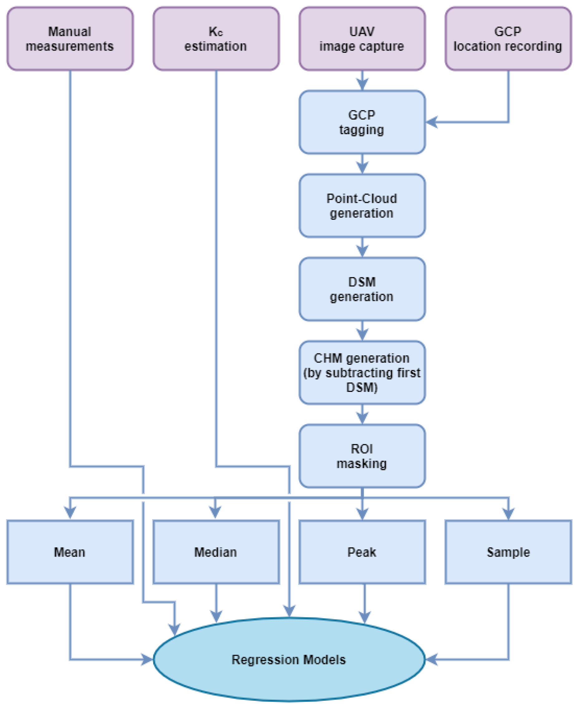A summary of the processing steps is presented in Figure 2.

2.3. K_c Estimation

The eddy-covariance method is one of the most accurate, direct, and defensible approaches for measuring field-scale crop evapotranspiration. The ET_c was measured in the Megido and Urim fields using the eddy-covariance method [19,20]. Reference evapotranspiration (ET₀) was calculated according to the FAO-56 Penman–Monteith method [16] based on meteorological data from a nearby meteorological station. The crop coefficient was then calculated as K_c = ET_c/ET₀. The daily K_c time series were smoothed using the spline method, and K_c values on survey days were extracted.

The experimental fields in Gadash farm were too small to measure K_c values in the same method because the eddy covariance footprint is larger than the experimental plots; therefore, they were estimated using a model calibrated previously in larger tomato fields using eddy covariance measurements to estimate K_c from satellite imagery [21]. Instead of using satellite imagery that is too coarse for this small plot, multispectral images were captured using a RedEdge-MX sensor (Micasense Inc., Seattle, WA, USA) mounted on a UAV during each survey and were used to derive vegetation indices (VIs). The K_c for each crop was estimated throughout the season based on the empirically derived relationship with VIs [16,17,18].

2.4. Orthomosaic Processing and CHM Calculation

Images from each flight were processed in Pix4Dmapper version 4.6.3 (Pix4D SA, Prilly, Switzerland), to create DSMs and orthomosaics. At least six images were marked manually for each GCP prior to processing in order to properly geo-locate the products. This process included creating a densified point cloud that has 3D location data.

The first flight in each field was conducted prior to planting or soon after, such that the resulting DSMs were used as a reference of the ground level. This reference of every field was subtracted from subsequent DSMs to create CHMs that represent the canopy height above ground.

The CHMs were masked by ROI polygons of the field around the area where the manual measurements were performed. Additional ROIs with reduced size were also tested in the potato experiments. The tomato experiments included different irrigation treatments; the ROIs created for this study represent two treatment blocks where manual height measurements were performed.

2.5. Height Derivation from CHMs

In order to compare the CHM heights to those measured manually, a single height value was extracted from each CHM. Four methods for this extraction were compared. The Mean method consisted of calculating the mean value of the CHM pixels in the ROI; the Median method consisted of calculating the median value of the CHM pixels in the ROI; the Peak method consisted of calculating the peak of the histogram of the CHM values in the ROI; and the Sample method consisted of calculating the mean value of pixels with the maximum value within 30 cm of 30 randomly selected points in the ROI. This sampling strategy is novel, to the best of our knowledge. The height values calculated by each method were compared to the mean of the manual measurements conducted on the same day and the daily K_c value by creating linear regression models for each crop. Outliers were identified by calculating z-scores for the regression residuals and omitting survey days with a score higher than 2 or lower than −2 before recalculating the linear model.

2.6. Geo-Located Measurements Experiment

Three UAV flights were conducted in a corn field in Gadash experimental farm in the Hula valley, Israel (33.184°N, 35.586°E; Figure 3). The first flight was conducted soon after planting while the soil was almost entirely bare and was used as a reference. The two subsequent flights were conducted after the corn was higher than 90 cm tall on average. On the days of the second and third flights, the heights of 40 plants were measured in the field using a handheld ruler, and the exact location was recorded using a RTK-GNSS device. The instruments and configurations of the UAV flights and the RTK-GNSS measurements were the same as in the aforementioned experiments, at a flight altitude of 20 m above ground.

DSMs and CHMs were created with the same method as previously described. Each manual measurement was compared to the CHM pixel value at the exact location. Linear regression models between ruler measurements and height estimations from the CHM were created for each date and combined data from both dates. Outliers were identified by calculating Z-scores for the regression residuals and omitting points with a score higher than 2 or lower than −2 before recalculating the linear model. This dataset was expected to produce the best performance because, unlike the field measurements in cotton, tomato, and potato, all height measurements in corn were geo-located, and the crop height was considerably larger than the measurement error. Accordingly, it represented the best performance that can be expected using this set of tools (i.e., UAV configurations, flight plans, and processing methodology).

3. Results

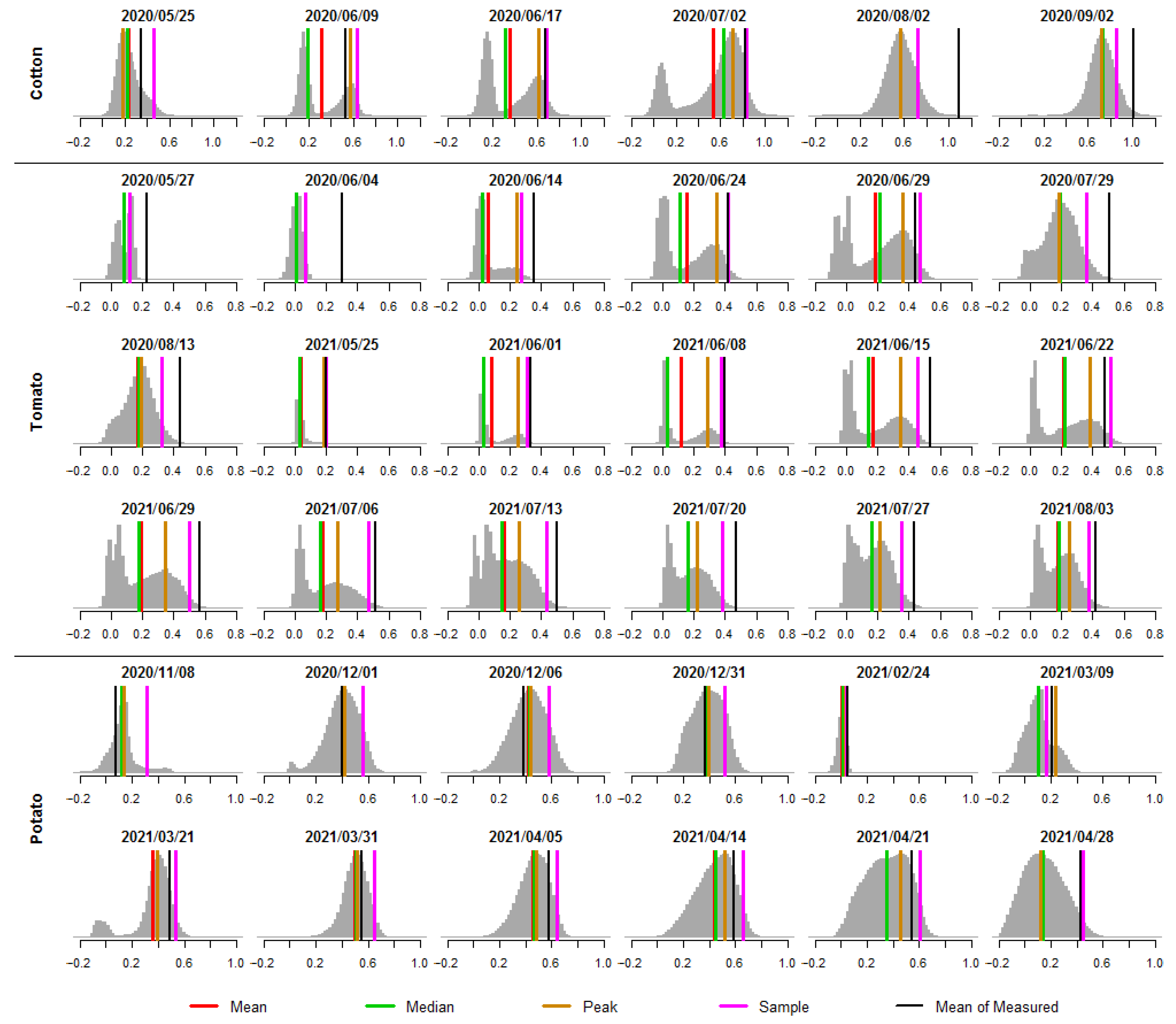
CHM histograms extracted from the ROIs are presented in Figure 4. Lines representing the values derived using different methods (Mean, Sample, Median, and Peak) are displayed on top of the histograms. The closer the derived value was to the measured value (marked with a black line), the better the method. On occasions with two peaks, the peak representing higher CHM values was chosen to calculate the crop height by the Peak method as the lower peak was assumed to represent bare soil. The Sample method values were consistently highest, followed most commonly by the Peak method, in all the CHMs across different crops. Figure 5 demonstrates that in tomatoes and cotton, the root mean square differences (RMSD) between manual measurements and CHM were most commonly lowest when using the Sample method, whereas the Peak method RMSD was most commonly lowest in potatoes.

One outlier for cotton (2020/08/02) was detected and removed from the height and K_c models, and an additional outlier (2020/09/02) was detected and removed from the K_c model alone. Three outliers for tomato were detected and removed only from the K_c models (2020/06/29, 2020/07/29, and 2020/08/13).

Figure 6 shows the linear regression models between the manual height measurements and the values derived from the CHMs by each of the four methods. Cotton height was most accurately estimated (RMSE = 0.056 m) by the Sample and Mean methods, which had the highest coefficient of determination (R² = 0.94). These two methods also achieved the best fit for tomatoes (R² = 0.73, 0.74 for Mean and Sample, respectively). All four methods achieved a similar performance for estimating potato height (R² = 0.82–0.84), whereas the Peak method yielded the lowest error (RMSE = 0.062 m). When mixing all crops, the Sample method showed the best fit (R² = 0.71). The ‘mixed’ models did not perform as accurately as the crop-specific models.

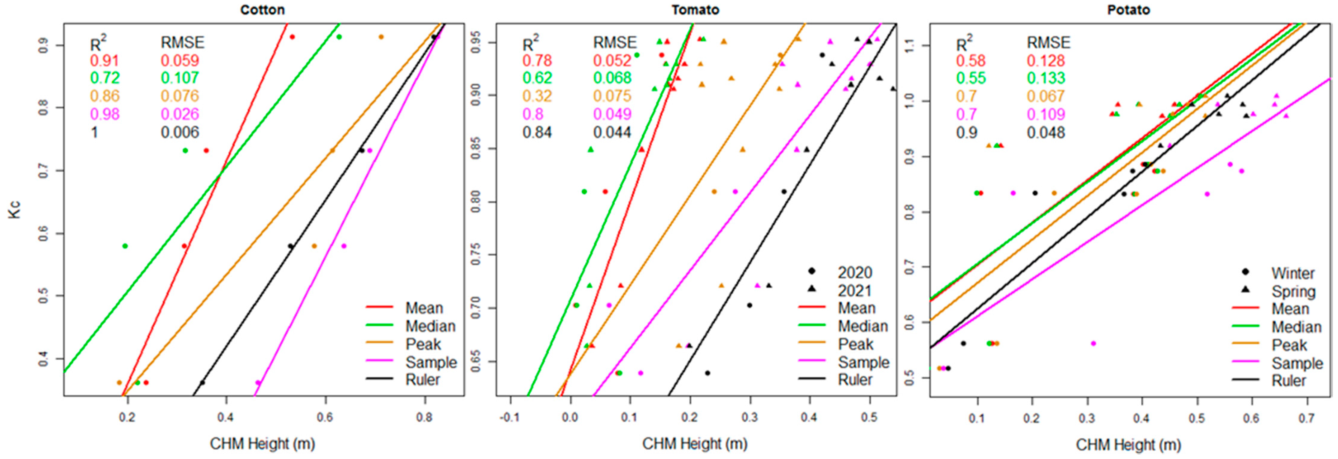
Linear regression models between K_c and the values derived from the CHMs by the four methods and the mean of the ruler measurements are presented in Figure 7. The Sample method performed best in cotton (R² = 0.98) and tomato (R² = 0.8). The Peak and Sample methods performed similarly for potato (R² = 0.7), although the error for the Peak method was smaller (RMSE = 0.067). The ruler measurements gave the best fit and error for all three crops. Because the ruler measurement were the best predictor for K_c, the methods that best estimated K_c from the CHM were those methods that best estimated the crop height.

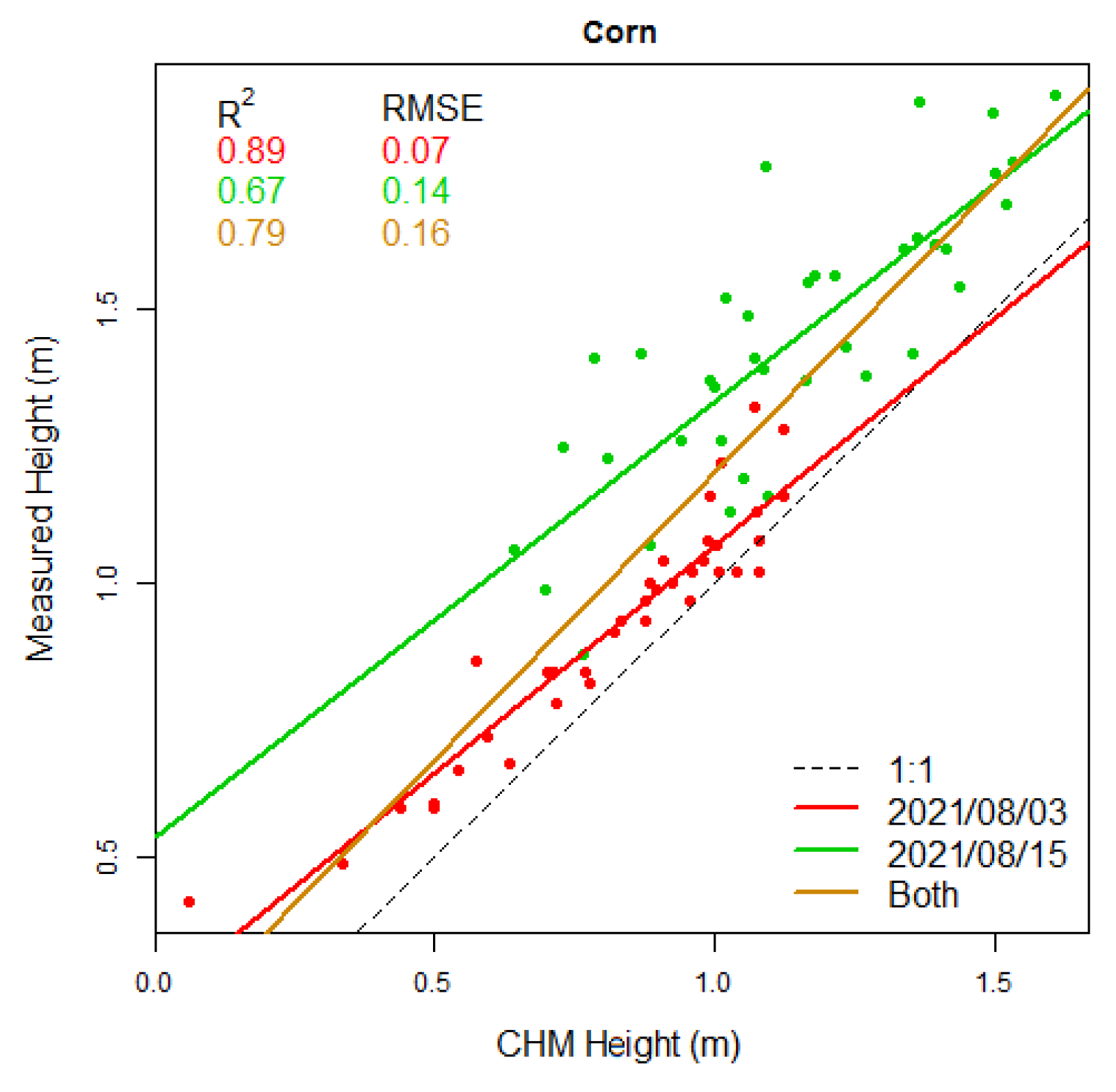
Two measurements in the first survey of the corn field were detected as outliers and removed. Linear regression models between the measured corn height and the geo-located values extracted from the CHMs are presented in Figure 8. The first survey yielded the best fit and the smallest error (R² = 0.89, RMSE = 0.07 m) and was closest to the 1:1 line, whereas the later survey gave a poorer result with double the error (R² = 0.67, RMSE = 0.14 m). This error might be because bent leaves were measured by the ruler rather than the corn tassel that had already developed in that stage. The model based on both surveys yielded a mediocre fit (R² = 0.79), but had the highest error (RMSE = 0.16 m).

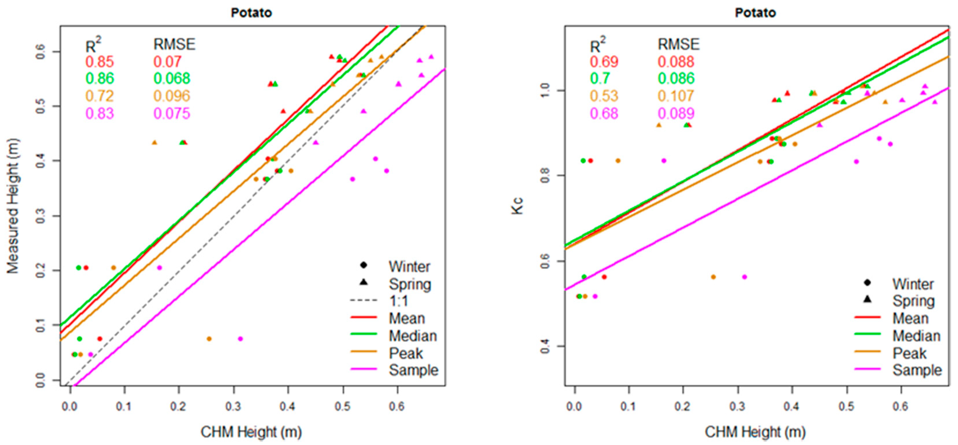
Linear regression models between manual height measurements, K_c, and the values derived from the CHMs by the four methods after reducing the size of the ROI in the potato fields are presented in Figure 9. A comparison of the fit and error is shown in

Table 2. Comparison of fit and error of the different models.

Model	Crop	ROI	Mean		Median		Peak		Sample
			R2	RMSE	R2	RMSE	R2	RMSE	R2	RMSE
Height	Cotton	Large	0.94	0.056	0.86	0.084	0.76	0.11	0.94	0.056
	Tomato	Large	0.74	0.051	0.56	0.066	0.17	0.08	0.73	0.052
	Potato	Large	0.84	0.071	0.84	0.072	0.82	0.062	0.83	0.075
		Reduced Size	0.85	0.07	0.86	0.068	0.72	0.096	0.83	0.075
Kc	Cotton	Large	0.91	0.059	0.72	0.107	0.86	0.076	0.98	0.026
	Tomato	Large	0.78	0.052	0.62	0.068	0.32	0.075	0.8	0.049
	Potato	Large	0.58	0.128	0.55	0.133	0.7	0.067	0.7	0.109
		Reduced Size	0.69	0.088	0.7	0.086	0.53	0.107	0.68	0.089

. The fit and the error for the height model did not meaningfully improve when the ROI size was reduced for all methods and worsened considerably for the Peak method (R² = 0.72, RMSE = 0.096 m). The error for the Median method also increased (RMSE = 0.096 m). The reduction of the ROI size affected the K_c models by improving the fit and error for the Mean and Median methods (R² = 0.69–0.7, RMSE = 0.086–0.088) and worsening them for the Peak method (R² = 0.53, RMSE = 0.107). The fit for the Sample method did not meaningfully change, although the error was reduced (RMSE = 0.089).

4. Discussion

This study compared different approaches to deriving a height from CHMs, including the novel Sample method. The Sample and Mean methods gave the best result for cotton and tomato crops. When using the large ROI, the Peak method gave the best results for potatoes, although the other methods’ performances were similar. Conversely, when using a smaller ROI, the Peak method performed the worst, and the Sample and the Mean methods performed similarly to the full ROI models. In the combined crops model, the Sample method gave the best results. However, mixing the different crops was not as accurate as the crop-specific models, and therefore should be avoided. These results imply that the Mean and Sample methods are best for the tested crops and that they are unaffected by the size of the ROI. These models are best to consider in future studies to create new models for other crops.

The use of maximum local height in the Sample method was chosen for SfM derived CHMs. Because the resolution of LiDAR is very high, local outliers can appear in the data. Therefore, in some work, the local height is calculated by a percentile of the data rather than the maximum. For instance, Madec et al. [14] calculated that 99.5% is the best percentile for extracting values from LiDAR CHMs. In SfM, such local outliers are not common, and using such a threshold will slightly underestimate the peak values; therefore, the local maximum is better suited.

The coefficient of determination of the geo-located corn was not higher than in models using the Sample method. However, the error for the geo-located model using both survey dates was greater than that of the Sample method for all crops. Accordingly, it is not necessarily an advantage to use an expensive RTK-GNSS device when collecting field data to create height models. The RTK-GNSS is still important to georeference the orthomosaics to allow multi-date comparisons.

The coefficient of determination and RMSE values achieved in this study are very good even compared to studies using LiDAR. A 2017 study modeled terrestrial LiDAR scans against ruler measurements of wheat 80–100 cm tall and achieved an R² = 0.9 and RMSE = 0.034 m [14]. This study provided a potato height model better than a 2019 study that employed a UAV-based LiDAR and achieved R² = 0.5 and RMSE = 0.12 m [9]. Therefore, relatively inexpensive equipment can acquire RGB imagery and deliver CHMs of comparable quality to the more expensive airborne LiDAR.

Although estimation of K_c using ruler measurements gave the most accurate results, this method is not efficient for capturing the spatial heterogeneity in the field. An assessment of K_c according to a CHM is therefore necessary. The method that performed best for estimating K_c in cotton and tomato was the new Sample method. Estimating potato K_c using the Sample and Peak methods resulted in the same coefficient of determination, but the RMSE for the Peak method was lower. The very high coefficient of determination in cotton may be attributed to the small sample size (n = 4) of the model, and more data should be collected to ensure its validity. Nonetheless, according to both height and K_c models, the higher the crop, the better the coefficient of determination of the models. This may be due to the consistency of error magnitude between manual and CHM heights, which becomes negligible relative to the crop height when the crop is higher.

The comparison of height-derived estimations of K_c and field-measured K_c in this study is particularly novel. El-Naggar et al. [18] estimated K_c using a combination of a VI and LiDAR height data, but compared it to standard tabulated recommendations by FAO-56. The estimated K_c did not match the tabulated data, probably due to the effects of heterogeneity of soil in the plot. The use of VIs to predict K_c has been much studied in the past [22]. A model combining VIs and height similar to that El-Naggar et al. should be further investigated using real-time K_c measurements.

The comparison between the four methods showed that the Sample method introduced here for the first time consistently gave reliable results. The Mean method sometimes performed similarly to the Sample method. Nevertheless, it is best to try multiple methods for each crop for verification. The change of ROI size did not affect the Sample method, although it largely affected the Peak method, which must be considered. Empirical K_c estimation models were created with a good fit. Further use of low-cost UAVs and SfM can help farmers assess the spatial variability of crop height and its irrigation needs.

One such use could inform cotton growers and facilitate the regulation of vegetative growth that can be at the expense of reproductive development. Cotton height maps can be used to adjust precision irrigation maps to compensate for vegetative growth. Alternatively, in rainfed cotton, where regulating the growth through irrigation is not possible, prescription maps for the application of growth inhibitors can rely on CHMs. Other abnormalities such as pests and diseases inhibiting crop development might be detected in CHMs and addressed locally and precisely. Therefore, future studies could benefit from CHMs to develop applications for precision agriculture.

5. Conclusions

• The novel Sample method performed very well for modelling heights in all three tested crops.
• A global model that can be used for different crops is not as robust as crop specific models.
• K_c was highly correlated to CHM. This can be used to help farmers make spatially aware irrigation decisions.