Abstract
The aim of this work is to study the zonally asymmetric stratopause that occurred in the Arctic winter of 2019/2020, when the polar vortex was particularly strong and there was no sudden stratospheric warming. Aura Microwave Limb Sounder temperature data were used to analyze the evolution of the stratopause with a particular focus on its zonally asymmetric wave 1 pattern. There was a rapid descent of the stratopause height below 50 km in the anticyclone region in mid-December 2019. The descended stratopause persisted until mid-January 2020 and was accompanied by a slow descent of the higher stratopause in the vortex region. The results show that the stratopause in this event was inclined and lowered from the mesosphere in the polar vortex to the stratosphere in the anticyclone. It was found that the vertical amplification of wave 1 between 50 km and 60 km closely coincides in time with the rapid stratopause descent in the anticyclone. Overall, the behavior contrasts with the situation during sudden stratospheric warmings when the stratopause reforms at higher altitudes following wave amplification events. We link the mechanism responsible for coupling between the vertical wave 1 amplification and this form of zonally asymmetric stratopause descent to the unusual disruption of the quasi-biennial oscillation that occurred in late 2019.
1. Introduction
The stratopause is the transition boundary which separates the stratosphere from mesosphere and is typically characterized by a temperature maximum in the middle atmosphere and by a reversal of the thermal lapse rate at around 50 km (~1 hPa) [1]. The temperature and height of the stratopause depend on latitude and season. During undisturbed conditions, the polar stratopause in winter is relatively higher and warmer than the adjacent midlatitude stratopause [2,3,4]. The polar stratopause becomes even warmer in summer, but lower in height [1,4,5]. In the polar winter, dynamical warming associated with planetary waves, particularly those of zonal wavenumber 1, plays an important role in temperature changes in the upper stratosphere and lower mesosphere [6] and, consequently, in the temperature and height of the stratopause [4]. On the other hand, it is noted that the polar stratopause in winter is higher and warmer than in midlatitudes due to the contribution from gravity wave driving of the mean meridional circulation and diabatic descent in the polar cap air [2,3,7].
The most famous stratospheric phenomenon in the Arctic is the sudden stratospheric warming (SSW), which is accompanied by a sharp increase in stratospheric temperature and a decrease in wind speed or even a wind reversal (westerly is changed to easterly) [3,8,9,10]. According to the activity in the spectral components of the planetary waves (PWs), SSW events can be divided into displacement events and splitting events. This division depends on the enhanced amplitude of the PW component with zonal wave number 1 or 2 (wave 1 or wave 2), respectively, which determine the dynamics of the stratospheric polar vortex [10,11,12]. In a wave 1 pattern, the vortex is displaced off the pole, and in a wave 2 pattern, the vortex is elongated and tends to split into two parts [4,9,13,14]. The propagation of planetary waves into the Arctic winter stratosphere is crucially influenced by the vertical structure of winds in the lower atmosphere, and particularly from the state of quasi-biennial oscillation (QBO) [15] which has been shown to produce regionally asymmetric wave forcing depending on its phase [16].
The stratospheric final warming (SFW) can be preceded by a non-SSW winter, and it differs in timing from that occurred after the SSW winter [17,18]. The dates of the boreal spring SFW events during 1979–2010 were defined as the time when the zonal-mean zonal wind at the central latitudes of the westerly polar jet (65–75°N) drops below zero and never recovers until the subsequent autumn [19]. Accompanying the SFW onset, the stratospheric circulation changes from a winter dynamical state to a summer state and the largest negative transformation of the zonal wind and the rapidly weakened planetary wave activity are observed [19]. In addition, the out-of-phase relationship of temperature anomalies between the stratosphere and the troposphere during the process of SFW events suggests a close dynamic coupling between the stratosphere and the troposphere in spring [20].
SSW are often associated with the events of ‘elevated stratopause’ (ES), when the stratopause over the polar cap first descends, then becomes indistinct, and finally reforms at a much higher altitude than normal [21,22]. The ES events can be accompanied by a nearly isothermal region between the stratosphere and the mesosphere [21]. Eixmann et al. [23] found that the local temperature of the stratopause at Andenes (69°N, 16°E) and Kühlungsborn (54°N, 11°E) can be explained by the variability of waves 1–3. The importance of the westward propagating PWs in the ES events was reported by Limpasuvan et al. [7].
Using the Specified Dynamics Whole Atmosphere Community Climate Model (SD-WACCM), Stray et al. [24] investigated the seven SSW events accompanied by ES events during the years 2000–2008. A significant enhancement in wave 1–2 amplitudes near 95 km was found to occur after the wind reversed at 50 km. Not all SSW events are accompanied by ES events [3,22] and the simulations also show that there is not a close correspondence between major SSW and ES [3]. The descent of the polar stratopause after it reforms at high altitude is accompanied by the enhanced downward transport and increase in the concentrations of the upper-stratospheric minor species, such as CO and NO, that have sources in the mesosphere [25,26,27,28,29]. Remsberg [30] analyzed the relationship between H2O and ozone and the temperature of the stratopause and noted that the increases in H2O and decreases in O3 cool the upper stratosphere.
The existence of a zonally asymmetric elevated stratopause was first emphasized in France et al. [1] and France and Harvey [31]. The effects of the zonal asymmetry in temperature and height of the stratopause with respect to the location of the polar vortices and anticyclones were considered [1,4,31,32]. Using Aura Microwave Limb Sounder (MLS) satellite data during 2004–2011, France et al. [1] found that both the highest and lowest stratopause temperatures are located near the vortex edge and the height of the stratopause in the cyclone is higher than in the anticyclone. Given the winter climatology, cyclonic circulation of the polar vortex and anticyclonic structure are more common around the Greenwich Meridian (0°E), and Aleutian High (~180°E), respectively [1,4,31,33].
In the recent Arctic winter, 2019/2020, an unusually strong, cold, and persistent polar vortex was formed [34], which was the most stable since the 2010/11 winter [35,36]. The vortex was not associated with an SSW event, but instead with a vortex split in April which was followed by an SFW in late April–May [18,37]. Due to zonal asymmetry of the polar vortex in spring 2020, the strongest ozone depletion and surface weather effects were also zonally asymmetric [18,37,38]. A further aspect of the conditions around this time was that the QBO displayed unusual behavior. The downward propagating transition from the westerly to the easterly phase that was underway was disrupted, particularly around the 30 hPa level from December 2019, with the QBO remaining westerly at this level for much of 2020 and tending to be easterly at lower and higher levels [39].
This paper is focused on the seasonal evolution of the zonally asymmetric stratopause in the non-SSW winter–spring of 2019/2020. In Section 2, data sources and analysis method are briefly described. Section 3 considers the variability of the zonal wind, polar temperature and amplitudes of wave 1 and wave 2, associated with the zonal asymmetry of the stratopause. The discussion is given in Section 4, and Section 5 provides a summary and conclusions.
2. Materials and Methods
The evolution of the Arctic stratopause in the non-SSW winter of 2019/2020 was analyzed using data from Aura MLS satellite observations and Modern-Era Retrospective Analysis for Research and Applications, Version 2 (MERRA-2) reanalysis data [40]. The temperature data from Aura MLS Version 4.2 [41,42,43] are used. The MLS temperature data covers the pressure level range of 316–0.01 hPa (about 8–80 km) with the vertical resolution ~2 km in the stratosphere and ~6 km in the mesosphere. In this case, when there is a null value in the dataset, a one-dimensional interpolation method was used.
Zonal wind and polar temperature were used from MERRA-2, which is the global reanalysis produced by the Goddard Earth Observing System (GEOS) covering the period from January 1980 to the present. The horizontal longitude × latitude resolution is 0.625° × 0.5°, the minimum time resolution is one hour, and the vertical stratification is 72 layers from the surface to 0.01 hPa [44]. The reanalysis data were obtained from the Goddard Earth Sciences Data and Information Services Center [40]. The temperature variations in time–altitude section from the 60–90°N mean data were analyzed using the National Oceanic and Atmospheric Administration National Centers for Environmental Prediction, Global Data Assimilation System–Climate Prediction Center at [45].
3. Results
3.1. Zonal Wind and Temperature Variability
The evolution of the Arctic polar vortex in winter–spring of 2019/2020 did not meet the major SSW criterion of Charlton and Polvani [9], since a zonal wind reversal at 10 hPa, 60°N, was not observed (Figure 1a). The vortex was strong during December–March with zonal wind speeds mostly in the range 40–60 ms–1, reaching a peak of 67 ms–1 in January (Figure 1a). Starting from the coldest polar cap temperature at 10 hPa in mid-December 2019, a slow warming tendency took place. It was accompanied by alternate short-term warming–cooling with three temperature peaks in January–April 2020 (Figure 1b).
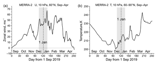
Figure 1.
MERRA-2 [40] data for (a) zonal wind at 10 hPa, 60°N and (b) polar temperature at 10 hPa, 60–90°N, in September 2019–April 2020. The gray rectangles show the time interval from mid-December to mid-January, which stands out in the variability of the zonally asymmetric stratopause (Section 3.2).
These peaks decreased in height as seen in the time–altitude section from GDAS-CPC data (black curve at −50 °C in Figure 2a). The MERRA-2 data show that the polar temperature distributions near the stratopause (50 km) in December–January were zonally asymmetric with a dominant wave 1 pattern (Figure 2b,c). The eastward rotation of the temperature field between December and January (Figure 2b,c) resulted in the location of high and low temperature regions almost along the meridians 0°E and 180°E in January (Figure 2c). This location corresponds to the Atlantic and Pacific sectors, respectively. Since the winter Arctic polar vortex was climatologically shifted from the North Pacific sector toward Atlantic–Eurasia [13,46], similar to asymmetry observed during the easterly QBO phase [16], we consider these two sectors with respect to the stratopause zonal asymmetry, which demonstrate similar patterns [1,4,31].
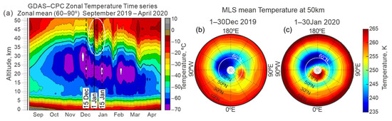
Figure 2.
(a) GDAS–CPC temperature variations in a time–altitude section from the 60–90°N mean in September–April 2019/2020 [45]. The black curve shows the vertical change in the −50 °C temperature contour and the white oval outlines the warming peak in early January 2020. Monthly mean MLS temperature [43] in the NH at the mean stratopause height (50 km) in (b) December 2019 and (c) January 2020.
3.2. Zonally Asymmetric Stratopause Variability
Based on Aura MLS data, we examine variability of the vertical temperature profile around 0°E and 180°E. Figure 3 shows time–altitude sections of the temperature at individual 5-degree zones centered at 60°N, 70°N and 80°N (Figure 3, from bottom to top). The stratopause in vertical temperature profile is defined by the temperature maximum between the stratosphere and the mesosphere [31]. The stratopause varies around its typical mean heights ~50 km at the edges of the time (horizontal) axis, in September and March (dashed curve in Figure 3e). In October–November, the temperature maximum elevates above this mean level, especially at the higher latitudes (middle and top panels). It covers a larger height range of 50–70 km in the polar vortex region (near 0°E, Figure 3f) than in the anticyclone region, 50–60 km (near 180°E, Figure 3e). Additionally, the stratopause elevates poleward between 60°N and 80°N in both sectors (Figure 3, bottom to top). The spatial patterns in both cases reflect the fact that the climatological stratopause is highest inside the polar vortex [31].
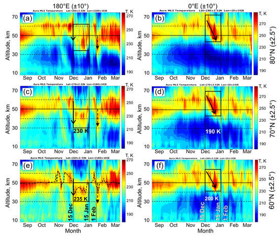
Figure 3.
Vertical temperature profiles from Aura MLS in September 2019–March 2020 at longitudes (a,c,e) 180 ± 10°E and (b,d,f) 0 ± 10°E for latitudes (e,f) 60 ± 2.5°N, (c,d) 70 ± 2.5°N, and (a,b) 80 ± 2.5°N. The time interval of the descending stratopause, 15 December–15 January, is indicated by vertical lines, and the temperature maximum is outlined by a rectangle. Arrows show tendencies in the decent of the temperature maximum. The thick solid line highlights the typical stratopause altitude of 50 km, and thin horizontal dashed lines are shown at 30, 40, and 60 km altitude. The thick dashed line in (e) shows the time-altitude evolution of the temperature maximum at the stratopause.
Different tendencies are observed in zonally asymmetric regions between mid-December and mid-January (vertical lines in Figure 3). The range of variability of the temperature maximum in the anticyclone region sharply descends in mid-December from 50–60 km to 30–50 km during one or two days (solid arrows and rectangles in Figure 3c,e). In the vortex region, the temperature maximum starts to slowly descend from ~60 km to ~45 km during a three week period (arrows and rectangles in Figure 3d,f). These examples characterize the latitudes 60°N and 70°N (Figure 3e,f and Figure 3c,d, respectively), which correspond to the average latitudinal locations of the polar vortex and anticyclone regions relative to the pole (red and blue areas, respectively, in Figure 2b,c). In particular, the time–altitude sections at 60°N in Figure 3e,f correspond to the edge region of the cyclonic polar vortex and the inner part of the anticyclone, respectively. This is generally consistent with the polar vortex and anticyclones climatology (e.g., [31]). Then, we can conclude that the stratopause near 15 December 2019 almost stepwise descended by 10–20 km in the anticyclone region (Figure 3, left, solid arrow and rectangle). Separate to this, it demonstrated a relatively monotonic lowering between ~60 km and ~50 km during three weeks in the vortex region (Figure 3, right, arrow and rectangle).
Between mid-December and mid-January, the temperature maximum in the anticyclone region was predominantly below 50 km and occupies middle–upper stratosphere (Figure 3c,e). At the same time, the temperature maximum in the vortex region was near and above 50 km, extending from upper stratosphere to mesosphere (Figure 3b,d,f). This is in general consistency with [1] that the stratopause in the Aleutian anticyclone is lower than in ambient air during the Arctic winter. Our results for the non-SSW winter 2019/2020 (Figure 3) mean that the stratopause sloped downward between the North Pacific and the North Atlantic, descending from the mesosphere to the stratosphere.
The zonal wind speed at 60°N, 10 hPa, continued to increase in mid-December to mid-January and reached a peak winter speed (Figure 1a). Simultaneously, the polar cap temperature started to rise (Figure 1b), indicating that seasonal stratospheric warming had begun. Neither time series show a clear consistency with temporal variations of the stratopause height. As noted above, stratospheric warming in the polar cap demonstrated a descending tendency in December–January by about 10 km for the temperature contour −50 °C (Figure 2a, black curve). Therefore, a decrease in height of the polar cap temperature (Figure 2a) was generally consistent with the zonally asymmetric descent of temperature maximum in December–January (Figure 3). However, the large-scale tendency does not explain the regional difference in changes in vertical temperature profiles. It should be emphasized again that a sequence of temperature peaks in the polar cap (Figure 1b and Figure 2a) do not correspond in time to the episodes of stratopause descent observed in zonally asymmetric regions in December and early February (arrows in Figure 3).
The temperature maximum in the horizontal plane was more compact in the cyclone region compared to the longitudinally extended temperature minimum in the anticyclone region (red and blue areas around the pole in Figure 2b,c). Between December and January, due to the eastward shift of the related temperature gradients toward the meridians 0°E–180°E, this could have contributed to sharper changes with time in the vertical profile in the cyclone region around 0°E than in the anticyclone region around 180°E. Nevertheless, Figure 3 shows that, on the contrary, descent in the cyclone region was more prolonged in time (arrows in right column).
Consequently, the temperature change in the polar region in the stratosphere (Figure 1b and Figure 2a) and in the geographic patterns at the mean stratopause height of 50 km (Figure 2b,c) cannot explain the difference in the zonally asymmetric features of the stratopause descent (Figure 3). In a search of the reasons for this difference, in Section 3.3 we compared the variability of the wave 1–2 amplitudes.
We note the existence of the zonally asymmetric temperature throughout the stratosphere. The middle stratosphere during December–January in the polar vortex was 35–40 K colder than in the anticyclone: 190–200 K versus 230–235 K, respectively (Figure 3). As noted in Section 1, the very cold polar vortex in winter 2019/2020 led to record low ozone in the Arctic, which was zonally asymmetric with an ozone minimum around 0°E (e.g., [38]).
3.3. Wave 1 and Wave 2 in the Upper Stratosphere and Lower Mesosphere
Considering the range of heights in the variability of the temperature maximum in Figure 3, the time series of the amplitudes of wave 1 and wave 2 at a mean stratopause height of 50 km was compared with those at 45 km, 55 km and 60 km (blue and red curves in Figure 4a–d). MLS temperature data at 60°N were used. It is known that planetary waves propagate upward with increasing amplitude, with wave 1 having larger amplitude than wave 2 [47,48,49] and their amplitudes anticorrelate in time [11,50]. The wave amplitudes at 50 km are somewhat lower than below at 45 km (compare Figure 4b and Figure 4a), but markedly increased above up to 60 km (Figure 4b–d), and the wave 1 amplitude was consistently larger than the wave 2 amplitude (blue and red curves in Figure 4a,b). The relative minimum of wave activity at 50 km (Figure 4b) is explained by the vertical structure of the wave 1–2 amplitudes according to the MLS temperature data for winter 2019/2020 (Figure 5). The largest amplitudes of both waves are in the stratosphere and mesosphere and are minimal around 50 km.
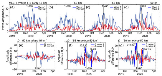
Figure 4.
Amplitudes of wave 1 and wave 2 at 60°N (a) below stratopause (45 km), (b) at mean climatological stratopause height (50 km), and (c,d) above stratopause (55 km, 60 km); (e–g) difference D between wave amplitude at (e) 50 km and 45 km, (f) 55 km and 50 km, and (g) 60 km and 50 km. Thickened parts of the blue (red) curve in (f) and (g) show rapid wave-1 (wave-2) amplitude increase (decrease) with altitude.
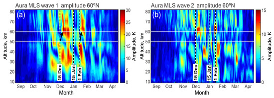
Figure 5.
Time–altitude section of amplitude of (a) wave 1 and (b) wave 2 at 60°N from the MLS temperature data. The time interval September 2019–April 2020 is presented. Arrows indicate cases of rapid vertical amplification of the wave 1 amplitude between 50 km and 60 km (white horizontal lines).
The wave amplitude variations are not evidently reflected in the stratopause changes. For example, the largest wave 1 peak near 1 January 2022 (Figure 4, blue curve in upper panel and vertical line on 1 January) was not accompanied by any response in the stratopause height (Figure 3). We found that wave amplitude change with height appears to be important. The difference D between the wave amplitudes at increasing heights between 45 km and 60 km was calculated (Figure 4, lower panel). The D time series show when the amplitude of each wave increases or decreases with height. Time series in Figure 4f (‘55 km minus 50 km’) and Figure 4g (‘60 km minus 50 km’) demonstrate a sharp vertical increase in wave 1 amplitude, starting from mid-December and early February (thickened parts of blue curve). Both events of vertical amplification of wave 1 above 50 km correspond to a downward stratopause jump in mid-December and early February (solid and dashed arrows, respectively, in Figure 3a,c,e). The D changes in wave 2 (thickened parts of red curve in Figure 4f,g) are antiphase and in magnitude and in mid-December are half as large as in wave 1. This relationship suggests the prevailing role of amplified wave 1 in the sharp stratopause descent (Figure 3, left). D-deviations in wave 1 below 50 km in each of the events are negative, differ greatly in magnitude (Figure 4e) and to some extent can also be involved in the development of stratopause descent. We further emphasize changes in D above 50 km (Figure 4f,g) as more consistent with the behavior of the stratopause in the Aleutian region (Figure 3, left).
We note that D in wave 1 above 50 km rapidly reverses from a large negative value to a large positive value in both events (Figure 4f,g). This means that initially the wave 1 amplitude is larger at 50 km than at 55 km and 60 km. The arrows in Figure 5a show that the wave 1 amplitude is high below and at 50 km and low just above 50 km. Then it becomes high again at 60 km in a few days. This results in the observed sharp changes in the sign of D in Figure 4f,g. Total changes in difference ‘60 km minus 50 km’ are D = 35 K around 15 December 2019 and D = 26 K around 1 February 2020 (Figure 4g).
These rapid changes in the sign and magnitude of D may play an important role in zonally asymmetric descents of the stratopause. A rapid vertical reversal of D (Figure 4f,g) occurs in the anticyclonic stratopause region (50–60 km in November–first half of December 2019; Figure 3, left) and can have a significant dynamical effect on the stratopause here. In the polar vortex, the stratopause variations occur at about 60 km and higher (Figure 3, right), where this effect apparently does not reach. Figure 3 and Figure 4, thus, show that the stratopause height in the Aleutian anticyclone is very sensitive to the rapid vertical amplification of wave 1 above the mean stratopause height ~50 km. It should be emphasized that the stratopause height in this region changes in antiphase with D. Such a clear dependence is not visible in the vortex region (Figure 3, right), where the stratopause descends slowly since mid-December 2019 and does not show any response to D in early February 2020.
4. Discussion
In this study, we have examined the zonally asymmetric stratopause variability over the Arctic in winter–spring 2019/2020, when no SSW events occurred. Zonal wind reversal, which is typical for the SSW, was not observed until the end of April (Figure 1a) and stratospheric final warming came in late April–May [18,37]. Due to the less-active upward propagation of planetary waves, the Arctic stratospheric polar vortex was exceptionally strong, cold, and persistent. This resulted in near-complete local reduction of stratospheric ozone [51] and the appearance of surface temperature anomalies in Eurasia and North America [52,53].
Although the upward planetary wave activity during winter 2019/2020 was smaller than the climatological average [37], zonal waves 1–2 showed variable amplitude in the stratosphere and mesosphere (Figure 4 and Figure 5). Several peaks in the stratospheric temperature of the polar cap (Figure 1b and Figure 2a) were associated with the wave 1 amplitude peaks in the stratosphere (Figure 4a). It is clear, however, that the polar cap-scale variability does not reflect many local or regional processes. We found a relationship between the asymmetry of the temperature field relative to the pole (Figure 2b,c), the height of the zonally asymmetric stratopause (Figure 3) and vertical increase in the wave 1 activity between 50 km and 60 km (Figure 4).
As noted in Section 1, the zonal asymmetry in the stratopause temperature and height depends on the location of polar vortices and anticyclones associated with wave 1 perturbation. On average, the stratopause in the polar cyclone is higher and warmer than in the anticyclone [1,4,31,32]. It is seen from Figure 2b,c that a clear temperature asymmetry relative to the pole in December 2019 and January 2020 was observed. The difference between the temperature maximum (warmer polar vortex) and the temperature minimum (colder Aleutian anticyclone) at the mean stratopause height 50 km was about 20 K.
Descent–ascent–descent of the polar stratopause usually occur during the onset and recovery phases of the SSW events, when the zonal wind at 60°N reverses to easterly and the polar vortex breaks down [4,21,22,32]. Special attention was paid to the elevated stratopause events characterized by a rapid reformation of the polar stratopause near 75–80 km and its subsequent gradual descent over a period of several weeks [3,7,23,32,54]. Due to the absence of the zonal wind reversal, this event is not typical for winter 2019/2020 (Figure 3).
In general, the stratopause shows a dependence on the planetary wave activity [22,23]. As is typical for the climatological wave 1 structure in winter stratopause [1,31], the stratopause height in polar vortex was persistently higher than in anticyclone (Figure 3, right and left, respectively). However, the wave 1 peaks in winter 2019/2020 (Figure 4, upper panel) did not associate with any anomalies in the stratopause (Figure 3). This is confirmed, in particular, by the absence of a stratopause response in Figure 3 to the largest peak of wave 1 near 1 January 2020, present in Figure 4a–d.
We emphasize that there was no zonal wind reversal (Figure 1a), vortex break down, or rapid stratopause reformation in the upper mesosphere (Figure 3) in non-SSW winter 2019/2020. The finding of this work is association of rapid stratopause descent in anticyclone with a rapid vertical increase in the wave 1 amplitude. The stratopause in the anticyclone before mid-December and in late January was somewhat elevated to ~60 km (Figure 3, left) relative to mean height of 50 km. This was the likely reason for the immediate response of the stratopause in this region in mid-December 2019 and early February 2020 (arrows in Figure 3, left) to rapid wave 1 amplification at the same height range (Figure 4f,g).
As far as we know, an almost stepwise and persistent descent of the stratopause in the anticyclone region (arrows in Figure 3, left) has not been previously described both in the SSW and non-SSW conditions. Determined from the zonal mean temperature, the stratopause descent in the SSW onset is short-term and is replaced by an elevation to the upper mesosphere [4,21,22,32]. The stratopause descent in late 2019–early 2020 (early February 2020) lasted for one month (a few days) and was replaced by the return of the stratopause to the initial height range. The slower stratopause descent to a normal height in Figure 3 (right) can be attributed to the persistently higher height of the temperature maximum (and stratopause) in the vortex region and the D-effect can be possibly less strong to cause rapid change in the temperature profile.
The disruption of the QBO in late 2019 that is noted in the Introduction was a special occurrence, and we are interested in what role, if any, this had on the stratopause asymmetry discussed above. The QBO disruption appears to have been triggered by momentum transport from the minor SSW that occurred in Southern Hemisphere during September 2019 [39]. Over the period from October 2019 to January 2020, there were increasing contributions to the overall disruption from wave activity originating in the tropics and Northern Hemisphere [55]. This event was only the second unusual cycling of the QBO observed; the previous event in February 2016 has been attributed to the influence of wave fluxes from the Northern Hemisphere mid-latitudes promoted by a strong El Niño event [56,57,58,59].
The stepwise descent of the stratopause in winter 2019/2020 was seen quite clearly, it was regionally localized inside the Aleutian anticyclone and was relatively long-lasing from mid-December to mid-January. The mechanism of its coupling with a rapid vertical amplification of wave 1 is not clear yet. However, it may relate to the persistence of the westerly QBO phase near 30 hPa which would tend to favor vertical wave propagation. The stratopause descent in the SSW onset phase is accompanied by strong tropospheric planetary wave forcing and the appearance of stratospheric easterlies [4,21,22]. It is possible that the wave 1 amplification in our results plays a role of similar dynamic forcing on the stratopause in the conditions of strong westerlies. The close coupling between vertical wave modification and zonally asymmetric stratopause evolution in non-SSW winter needs detailed study with more observational statistics and modeling.
5. Conclusions
Aura MLS temperature data were used to analyze the Arctic stratopause evolution in non-SSW winter 2019/2020 with a particular focus on its zonally asymmetric wave 1 pattern. The results show that the temperature maximum, which reflects the height of the stratopause, has undergone changes that are not associated with variations in the zonal wind, temperature of the polar cap, and wave 1–2 amplitudes.
The higher (lower) stratopause in the polar vortex (anticyclone) region showed slow (step-wise) descents in mid-December 2019 and early February 2020. These two events reveal interesting features of the zonally asymmetric stratopause under conditions of a strong polar vortex, which, in our opinion, have not been previously described.
In order to search for the causes of these features, the amplitudes of wave 1 and wave 2 from the Aura MLS temperature data in the upper stratosphere–lower mesosphere were compared. It was found that the vertical amplification of wave 1 between 50 km and 60 km closely coincides in time with the events of the rapid stratopause descent in the anticyclone region. This could relate to the persistence of the westerly QBO phase in the lower stratosphere which would tend to favor propagation of wave 1. Wave 2, which has much lower amplitude, but coupled with wave 1 due to anticorrelation, can also be partially involved in these events.
In the event from mid-December 2019 to mid-January 2020, the temperature maximum in the anticyclone was consistently within the range from 30 km to 50 km. In contrast, the maximum temperature decreased from about 60 km to about 50 km in the polar vortex. This means that the stratopause was tilted, descending from the mesosphere above the polar vortex to the stratosphere above the anticyclone. The mechanism responsible for coupling between the vertical wave 1 amplification and zonally asymmetric stratopause descent in the conditions of strong polar vortex and absence of the SSW has not yet been clarified and remains to be uncovered and detailed in future studies.
Author Contributions
Conceptualization, O.E. and G.M.; methodology, O.E., A.K. and Y.S.; data acquisition, Y.S. and O.E.; software, Y.A., C.Z., O.I. and O.E.; validation, O.E., Y.S., A.K. and G.M.; investigation, O.E., G.M., A.K. and Y.S.; writing—original draft preparation, O.E., A.K. and G.M.; writing—review and editing, O.E., C.Z., Y.S., G.M., Y.A., O.I. and V.S.; visualization, O.E. and Y.S.; supervision, G.M.; project administration, G.M., V.S. and W.H. Each author contributed to the interpretation and discussion of the results and edited the manuscript. All authors have read and agreed to the published version of the manuscript.
Funding
This research received no external funding.
Institutional Review Board Statement
The study did not require ethical approval.
Informed Consent Statement
Not applicable.
Data Availability Statement
The study did not report any data except for those references to which are already given in the text and in the reference list.
Acknowledgments
This work was partially supported by the College of Physics, International Center of Future Science, Jilin University, China, and by the Ministry of Education and Science of Ukraine with the grant BN-06 for prospective development of a scientific direction “Mathematical sciences and natural sciences” and the project 20BF051-02 at Taras Shevchenko National University of Kyiv. This work contributed to the National Antarctic Scientific Center of Ukraine research objectives, and contributed to Project 4293 of the Australian Antarctic Program. The MERRA-2 global reanalysis and Aura Microwave Limb Sounder (MLS) data were obtained from the Goddard Earth Sciences Data and Information Services Center. The temperature mean data were obtained from the National Oceanic and Atmospheric Administration National Centers for Environmental Prediction, Global Data Assimilation System–Climate Prediction Center.
Conflicts of Interest
The authors declare no conflict of interest.
References
- France, J.A.; Harvey, V.L.; Randall, C.E.; Hitchman, M.H.; Schwartz, M.J. A climatology of stratopause temperature and height in the polar vortex and anticyclones. J. Geophys. Res. Atmos. 2012, 117, D06116. [Google Scholar] [CrossRef]
- Hitchman, M.H.; Gille, J.C.; Rodgers, C.D.; Brasseur, G. The separated polar winter stratopause: A gravity wave driven climatological feature. J. Atmos. Sci. 1989, 46, 410–422. [Google Scholar] [CrossRef][Green Version]
- de la Torre, L.; Garcia, R.R.; Barriopedro, D.; Chandran, A. Climatology and characteristics of stratospheric sudden warmings in the Whole Atmosphere Community Climate Model. J. Geophys. Res. Atmos. 2012, 117, D04110. [Google Scholar] [CrossRef]
- Vignon, E.; Mitchell, D.M. The stratopause evolution during different types of sudden stratospheric warming event. Clim. Dyn. 2015, 44, 3323–3337. [Google Scholar] [CrossRef]
- Gerding, M.; Hoffner, J.; Lautenbach, J.; Rauthe, M.; Lubken, F.J. Seasonal variation of nocturnal temperatures between 1 and 105 km altitude at 54 degrees N observed by lidar. Atmos. Chem. Phys. 2008, 8, 7465–7482. [Google Scholar] [CrossRef]
- Rind, D.; Shindell, D.; Lonergan, P.; Balachandran, N.K. Climate change and the middle atmosphere. Part III: The doubled CO2 climate revisited. J. Clim. 1998, 11, 876–894. [Google Scholar] [CrossRef]
- Limpasuvan, V.; Orsolini, Y.J.; Chandran, A.; Garcia, R.R.; Smith, A.K. On the composite response of the MLT to major sudden stratospheric warming events with elevated stratopause. J. Geophys. Res. Atmos. 2016, 121, 4518–4537. [Google Scholar] [CrossRef]
- Charlton, A.J.; Polvani, L.M.; Perlwitz, J.; Sassi, F.; Manzini, E.; Shibata, K.; Pawson, S.; Nielsen, J.E.; Rind, D. A new look at stratospheric sudden warmings. Part II: Evaluation of numerical model simulations. J. Clim. 2007, 20, 470–488. [Google Scholar] [CrossRef]
- Charlton, A.J.; Polvani, L.M. A new look at stratospheric sudden warmings. Part I: Climatology and modeling benchmarks. J. Clim. 2007, 20, 449–469. [Google Scholar] [CrossRef]
- Ayarzagüena, B.; Palmeiro, F.M.; Barriopedro, D.; Calvo, N.; Langematz, U.; Shibata, K. On the representation of major stratospheric warmings in reanalyses. Atmos. Chem. Phys. 2019, 19, 9469–9484. [Google Scholar] [CrossRef]
- Labitzke, K. Interannual variability of the winter stratosphere in the Northern Hemisphere. Mon. Weather Rev. 1977, 105, 762–770. [Google Scholar] [CrossRef]
- Labitzke, K.; Naujokat, B. The lower Arctic stratosphere in winter since 1952. In SPARC Newsletter; World Climate Research Programme SPARC Office: Zurich, Switzerland, 2000; Volume 15, pp. 11–14. Available online: https://www.sparc-climate.org/publications/newsletter/ (accessed on 14 December 2021).
- Waugh, D.W.; Randel, W.J. Climatology of Arctic and Antarctic polar vortices using elliptical diagnostics. J. Atmos. Sci. 1999, 56, 1594–1613. [Google Scholar] [CrossRef]
- Lawrence, Z.D.; Manney, G.L. Does the Arctic stratospheric polar vortex exhibit signs of preconditioning prior to sudden stratospheric warmings? J. Atmos. Sci. 2020, 77, 611–632. [Google Scholar] [CrossRef]
- Baldwin, M.P.; Gray, L.J.; Dunkerton, T.J.; Hamilton, K.; Haynes, P.H.; Randel, W.J.; Holton, J.R.; Alexander, M.J.; Hirota, I.; Horinouchi, T.; et al. The quasi-biennial oscillation. Rev. Geophys. 2001, 39, 179–229. [Google Scholar] [CrossRef]
- Zhang, J.; Xie, F.; Ma, Z.; Zhang, C.; Xu, M.; Wang, T.; Zhang, R. Seasonal evolution of the quasi-biennial oscillation impact on the Northern Hemisphere polar vortex in winter. J. Geophys. Res. Atmos. 2019, 124, 12568–12586. [Google Scholar] [CrossRef]
- Hu, J.; Ren, R.; Yu, Y.; Xu, H. The boreal spring stratospheric final warming and its interannual and interdecadal variability. Sci. China Earth Sci. 2014, 57, 710–718. [Google Scholar] [CrossRef]
- Curbelo, J.; Chen, G.; Mechoso, C.R. Lagrangian analysis of the northern stratospheric polar vortex split in April 2020. Geophys. Res. Lett. 2021, 48, e2021GL093874. [Google Scholar] [CrossRef]
- Hu, J.; Ren, R.; Xu, H. Occurrence of winter stratospheric sudden warming events and the seasonal timing of spring stratospheric final warming. J. Atmos. Sci. 2014, 71, 2319–2334. [Google Scholar] [CrossRef]
- Hu, J.; Ren, R.; Xu, H.; Yang, S. Seasonal timing of stratospheric final warming associated with the intensity of stratospheric sudden warming in preceding winter. Sci. China Earth Sci. 2015, 58, 615–627. [Google Scholar] [CrossRef]
- Manney, G.L.; Kirstin, K.; Pawson, S.; Minschwaner, K.; Schwartz, M.J.; Daffer, W.H.; Livesey, N.J.; Mlynczak, M.G.; Remsberg, E.E.; Russell, J.M.; et al. The evolution of the stratopause during the 2006 major warming: Satellite data and assimilated meteorological analyses. J. Geophys. Res. Atmos. 2008, 113, D11115. [Google Scholar] [CrossRef]
- Chandran, A.; Collins, R.L.; Garcia, R.R.; Marsh, D.R.; Harvey, V.L.; Yue, J.; de la Torre, L. A climatology of elevated stratopause events in the whole atmosphere community climate model. J. Geophys. Res. Atmos. 2013, 118, 1234–1246. [Google Scholar] [CrossRef]
- Eixmann, R.; Matthias, V.; Höffner, J.; Baumgarten, G.; Gerding, M. Local stratopause temperature variabilities and their embedding in the global context. Ann. Geophys. 2020, 38, 373–383. [Google Scholar] [CrossRef]
- Stray, N.H.; Orsolini, Y.J.; Espy, P.J.; Limpasuvan, V.; Hibbins, R.E. Observations of planetary waves in the mesosphere-lower thermosphere during stratospheric warming events. Atmos. Chem. Phys. 2015, 15, 4997–5005. [Google Scholar] [CrossRef]
- Manney, G.L.; Daffer, W.H.; Strwbridge, K.B.; Walker, K.A.; Boone, C.D.; Bernath, P.F.; Kerzenmacher, T.; Schwartz, M.J.; Strong, K.; Sica, R.J.; et al. The high Arctic in extreme winters: Vortex, temperature, and MLS and ACE-FTS trace gas evolution. Atmos. Chem. Phys. 2008, 8, 505–522. [Google Scholar] [CrossRef]
- Manney, G.L.; Schwartz, M.J.; Krüger, K.; Santee, M.L.; Pawson, S.; Lee, J.N.; Daffer, W.H.; Fuller, R.A.; Livesey, N.J. Aura Microwave Limb Sounder observations of dynamics and transport during the record-breaking 2009 Arctic stratospheric major warming. Geophys. Res. Lett. 2009, 36, L12815. [Google Scholar] [CrossRef]
- Marsh, D.R. Chemical–dynamical coupling in the mesosphere and lower thermosphere. In Aeronomy of the Earth’s Atmosphere and Ionosphere; Abdu, M., Pancheva, D., Eds.; IAGA Special Sopron Book Series; Springer: Dordrecht, The Netherlands, 2011; Volume 2. [Google Scholar] [CrossRef]
- Smith, A.K.; Garcia, R.R.; Marsh, D.R.; Richter, J.H. WACCM simulations of the mean circulation and trace species transport in the winter mesosphere. J. Geophys. Res. Atmos. 2011, 116, D20115. [Google Scholar] [CrossRef]
- Wang, Y.; Shulga, V.; Milinevsky, G.; Patoka, A.; Evtushevsky, O.; Klekociuk, A.; Han, W.; Grytsai, A.; Shulga, D.; Myshenko, V.; et al. Winter 2018 major sudden stratospheric warming impact on midlatitude mesosphere from microwave radiometer measurements. Atmos. Chem. Phys. 2019, 19, 10303–10317. [Google Scholar] [CrossRef]
- Remsberg, E. Observation and attribution of temperature trends near the stratopause from HALOE. J. Geophys. Res. Atmos. 2019, 124, 6600–6611. [Google Scholar] [CrossRef]
- France, J.A.; Harvey, V.L. A climatology of the stratopause in WACCM and the zonally asymmetric elevated stratopause. J. Geophys. Res. Atmos. 2013, 118, 2241–2254. [Google Scholar] [CrossRef]
- García-Comas, M.; Funke, B.; López-Puertas, M.; González-Galindo, F.; Kiefer, M.; Höpfner, M. First detection of a brief mesoscale elevated stratopause in very early winter. Geophys. Res. Lett. 2020, 47, e2019GL086751. [Google Scholar] [CrossRef]
- Harvey, V.L.; Randall, C.E.; Goncharenko, L.; Becker, E.; France, J. On the upward extension of the polar vortices into the mesosphere. J. Geophys. Res. Atmos. 2018, 123, 9171–9191. [Google Scholar] [CrossRef]
- Varotsos, C.A.; Efstathiou, M.N.; Christodoulakis, J. The lesson learned from the unprecedented ozone hole in the Arctic in 2020; A novel nowcasting tool for such extreme events. J. Atmos. Sol.-Terr. Phys. 2020, 207, 105330. [Google Scholar] [CrossRef]
- Lawrence, Z.D.; Perlwitz, J.; Butler, A.H.; Manney, G.L.; Newman, P.A.; Lee, S.H.; Nash, E.R. The remarkably strong Arctic stratospheric polar vortex of winter 2020: Links to record-breaking Arctic Oscillation and ozone loss. J. Geoph. Res. Atmos. 2020, 125, e2020JD033271. [Google Scholar] [CrossRef]
- Varotsos, C.A.; Cracknell, A.P.; Tzanis, C. The exceptional ozone depletion over the Arctic in January–March 2011. Remote Sens. Lett. 2012, 3, 343–352. [Google Scholar] [CrossRef]
- Zhang, Y.; Cai, Z.; Liu, Y. The exceptionally strong and persistent Arctic stratospheric polar vortex in the winter of 2019–2020. Atmos. Ocean. Sci. Lett. 2021, 14, 100035. [Google Scholar] [CrossRef]
- Inness, A.; Chabrillat, S.; Flemming, J.; Huijnen, V.; Langenrock, B.; Nicolas, J.; Polichtchouk, I.; Razinger, M. Exceptionally low Arctic stratospheric ozone in spring 2020 as seen in the CAMS reanalysis. J. Geophys. Res. Atmos. 2020, 125, e2020JD033563. [Google Scholar] [CrossRef]
- Anstey, J.A.; Banyard, T.P.; Butchart, N.; Coy, L.; Newman, P.A.; Osprey, S.; Wright, C.J. Prospect of increased disruption to the QBO in a changing climate. Geophys. Res. Lett. 2021, 48, e2021GL093058. [Google Scholar] [CrossRef]
- MERRA-2: The Goddard Earth Sciences Data and Information Services Center. Available online: https://gmao.gsfc.nasa.gov/reanalysis/MERRA-2/ (accessed on 15 July 2021).
- Livesey, N.J.; Read, W.G.; Wagner, P.A.; Froidevaux, L.; Lambert, A.; Manney, G.L.; Millán Valle, L.F.; Pumphrey, H.C.; Santee, M.L.; Schwartz, M.J.; et al. EOS MLS Version 4.2x–3.1 Level 2 Data Quality and Description Document, Tech. Rep., Jet Propulsion Laboratory. 2018. Available online: https://mls.jpl.nasa.gov/data/v4-2_data_quality_document.pdf (accessed on 12 January 2022).
- Schwartz, M.; Livesey, N.; Read, W. MLS/Aura Level 2 Geopotential Height V004, Greenbelt, MD, USA, Goddard Earth Sciences Data and Information Services Center (GES DISC) 2015a. 2015. Available online: https://disc.gsfc.nasa.gov/datasets/ML2GPH_004/summary/ (accessed on 15 July 2021).
- Schwartz, M.; Livesey, N.; Read, W. MLS/Aura Level 2 Temperature V004, Greenbelt, MD, USA, Goddard Earth Sciences Data and Information Services Center (GES DISC) 2015b. 2015. Available online: https://disc.gsfc.nasa.gov/datasets/ML2T_004/summary?keywords=temperature (accessed on 15 December 2021).
- Gelaro, R.; McCarty, W.; Suárez, M.J.; Todling, R.; Molod, A.; Takacs, L.; Randles, C.A.; Darmenov, A.; Bosilovich, M.G.; Reichle, R.; et al. The Modern-Era Retrospective Analysis for Research and Applications, Version 2 (MERRA-2). J. Clim. 2017, 30, 5419–5454. [Google Scholar] [CrossRef]
- GDAS–CPC: The National Oceanic and Atmospheric Administration National Centers for Environmental Prediction, Global Data Assimilation System–Climate Prediction Center (NOAA NCEP GDAS–CPC). Stratosphere-Troposphere Monitoring. Available online: https://www.cpc.ncep.noaa.gov/products/stratosphere/strat-trop/ (accessed on 15 December 2021).
- Karpetchko, A.; Kyrö, E.; Knudsen, B.M. Arctic and Antarctic polar vortices 1957–2002 as seen from the ERA-40 reanalyses. J. Geophys. Res. Atmos. 2005, 110, D21109. [Google Scholar] [CrossRef]
- Charney, J.G.; Drazin, P.G. Propagation of planetary-scale disturbances from the lower into the upper atmosphere. J. Geophys. Res. 1961, 66, 83–109. [Google Scholar] [CrossRef]
- Matsuno, T. Vertical propagation of stationary planetary waves in the winter Northern Hemisphere. J. Atmos. Sci. 1970, 27, 871–883. [Google Scholar] [CrossRef]
- Shi, Y.; Evtushevsky, O.; Shulga, V.; Milinevsky, G.; Klekociuk, A.; Andrienko, Y.; Han, W. Mid-Latitude mesospheric zonal wave 1 and wave 2 in recent boreal winters. Remote Sens. 2021, 13, 3749. [Google Scholar] [CrossRef]
- Smith, A.K. Observations of wave–wave interactions in the stratosphere. J. Atmos. Sci. 1983, 40, 2484–2496. [Google Scholar] [CrossRef]
- Wohltmann, I.; von der Gathen, P.; Lehmann, R.; Maturilli, M.; Deckelmann, H.; Manney, G.L.; Davies, J.; Tarasick, D.; Jepsen, N.; Kivi, R.; et al. Near-complete local reduction of Arctic stratospheric ozone by severe chemical loss in spring 2020. Geophys. Res. Lett. 2020, 47, e2020GL089547. [Google Scholar] [CrossRef]
- Zhang, J.; Lin, D.; Bian, J.; Xuan, T.; Chen, H.; Bai, Z.; Wan, X.; Zheng, X.; Xia, X.; Lyn, D. Long-term ozone variability in the vertical structure and integrated column over the North China Plain: Results based on ozonesonde and Dobson measurements during 2001-2019. Environ. Res. Lett. 2021, 16, 074053. [Google Scholar] [CrossRef]
- Xia, Y.; Hu, Y.; Zhang, J.; Xie, F.; Tian, W. Record Arctic ozone loss in spring 2020 is likely caused by North Pacific warm sea surface temperature anomalies. Adv. Atmos. Sci. 2021, 38, 1723–1736. [Google Scholar] [CrossRef]
- Scheffler, J.; Ayarzagüena, B.; Orsolini, Y.J.; Langematz, U. Elevated stratopause events in the current and a future climate: A chemistry-climate model study. J. Atmos. Sol.-Terr. Phys. 2022, 227, 105804. [Google Scholar] [CrossRef]
- Kang, M.-J.; Chun, H.-Y. Contributions of equatorial waves and small-scale convective gravity waves to the 2019/20 quasi-biennial oscillation (QBO) disruption. Atmos. Chem. Phys. 2021, 21, 9839–9857. [Google Scholar] [CrossRef]
- Coy, L.; Newman, P.A.; Pawson, S.; Lait, L.R. Dynamics of the Disrupted 2015/16 quasi-biennial oscillation. J. Clim. 2017, 30, 5661–5674. [Google Scholar] [CrossRef]
- Dunkerton, T.J. The quasi-biennial oscillation of 2015–2016: Hiccup or death spiral? Geophys. Res. Lett. 2016, 43, 10547–10552. [Google Scholar] [CrossRef]
- Kang, M.-J.; Chun, H.-Y.; Garcia, R.R. Role of equatorial waves and convective gravity waves in the 2015/16 quasi-biennial oscillation disruption. Atmos. Chem. Phys. 2020, 20, 14669–14693. [Google Scholar] [CrossRef]
- Varotsos, C.; Sarlis, N.V.; Efstathiou, M.N. On the association between the recent episode of the quasi-biennial oscillation and the strong El Niño event. Theor. Appl. Climatol. 2018, 133, 569–577. [Google Scholar] [CrossRef]
Publisher’s Note: MDPI stays neutral with regard to jurisdictional claims in published maps and institutional affiliations. |
© 2022 by the authors. Licensee MDPI, Basel, Switzerland. This article is an open access article distributed under the terms and conditions of the Creative Commons Attribution (CC BY) license (https://creativecommons.org/licenses/by/4.0/).