
Simulation of the Radar Cross Section of a Noctuid Moth

 , , and
Abstract
:1. Introduction
2. Materials and Methods
2.1. Overview
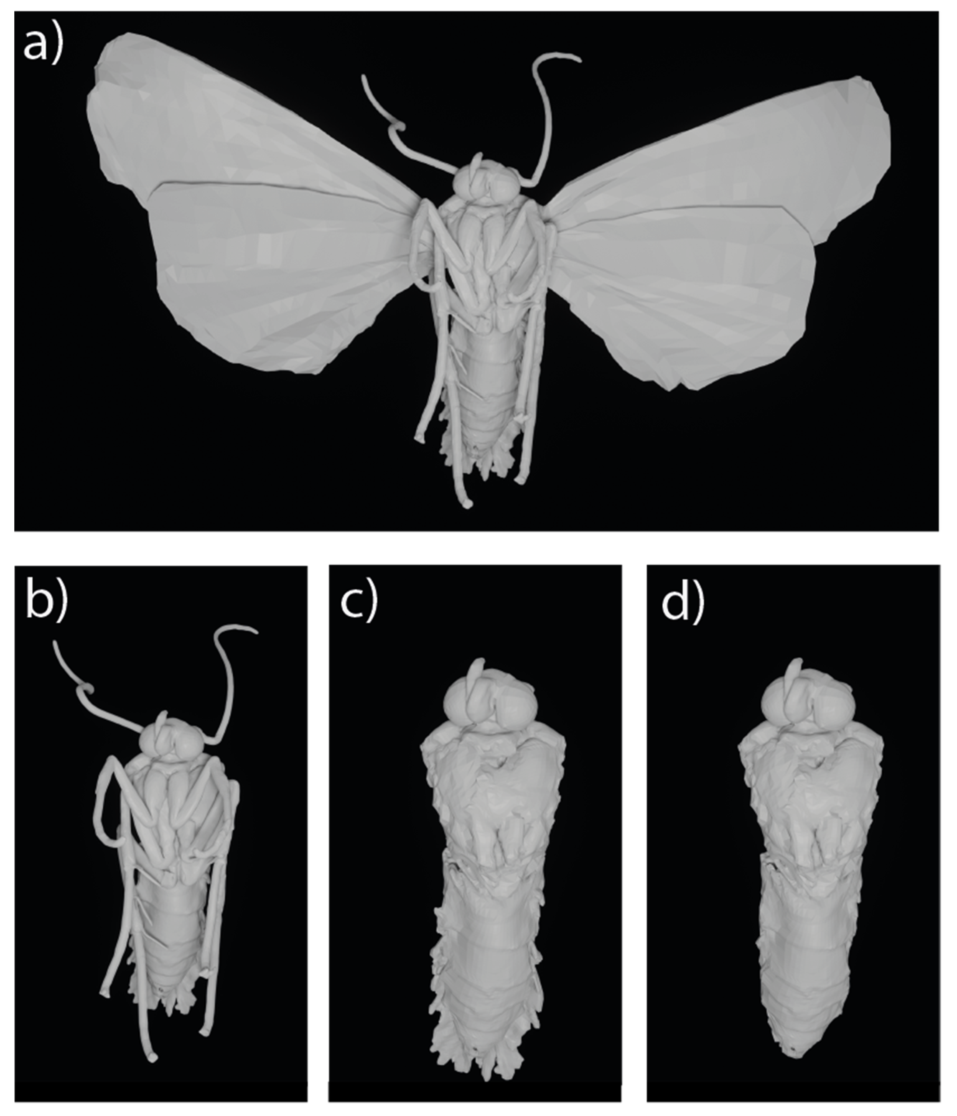
2.2. Description of the Specimen
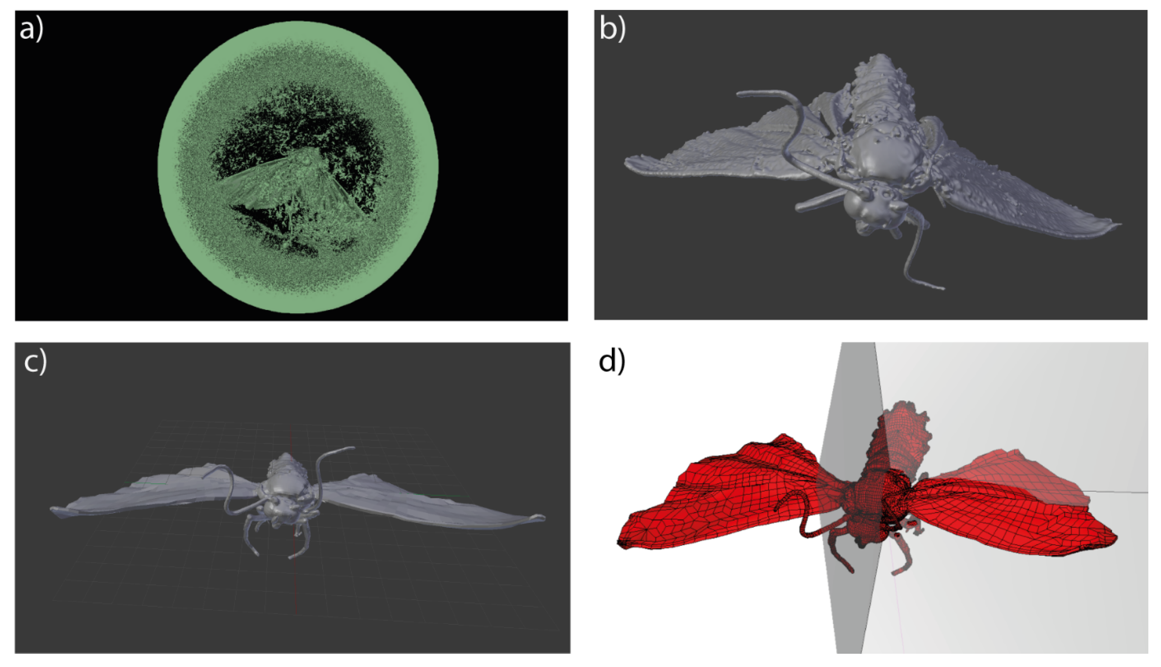
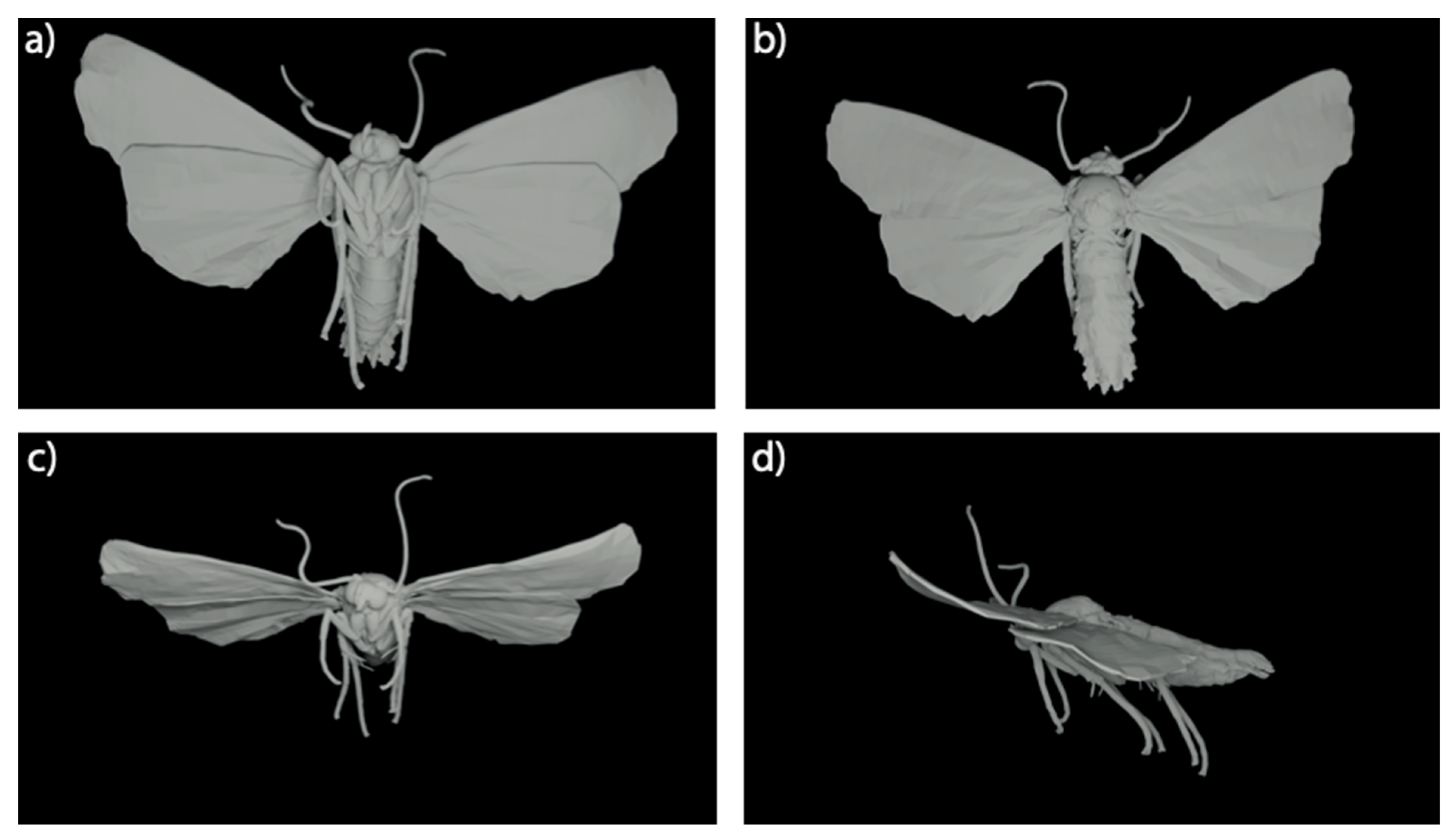
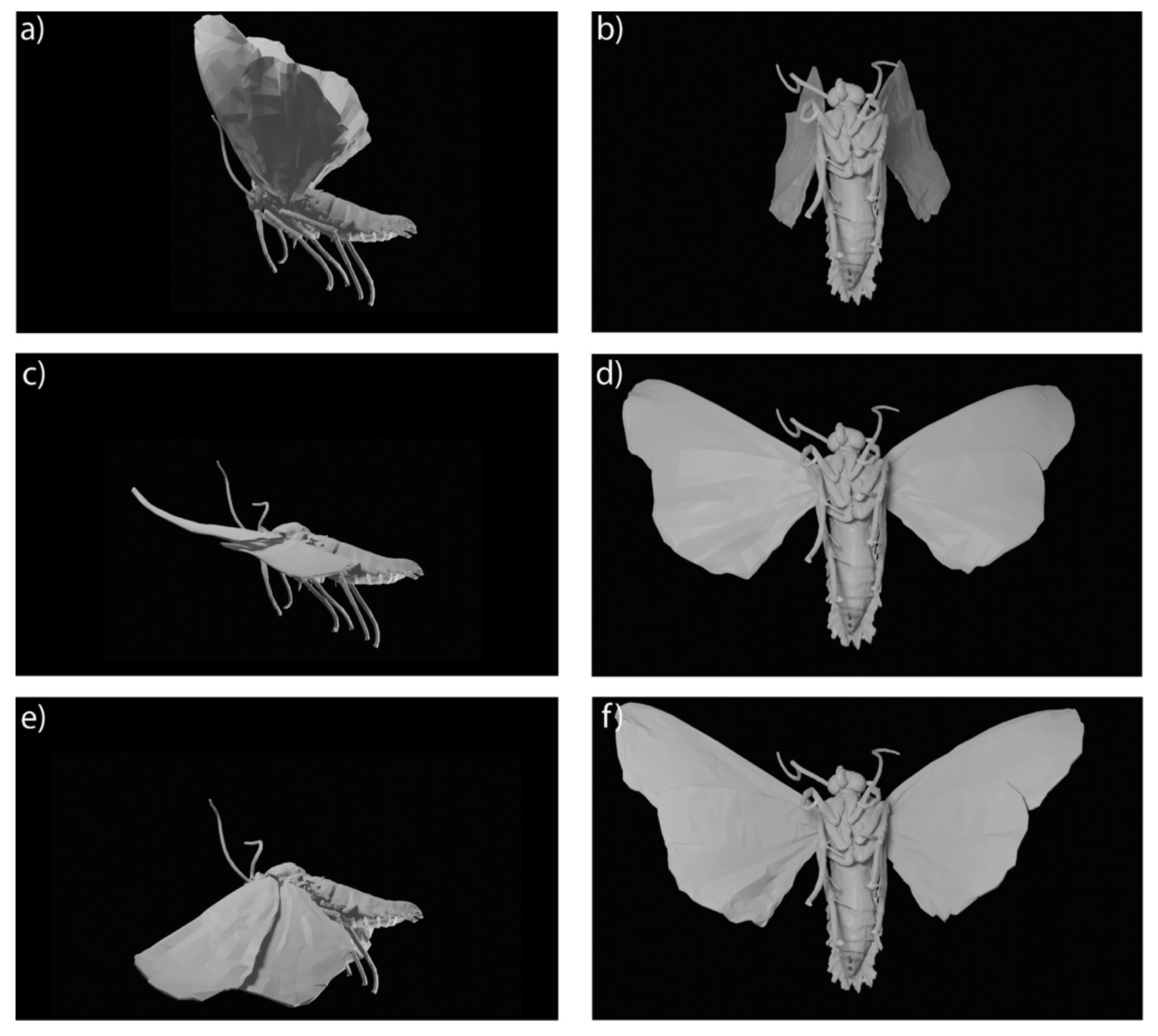
2.3. 3D Modelling
2.4. Electromagnetic Simulations
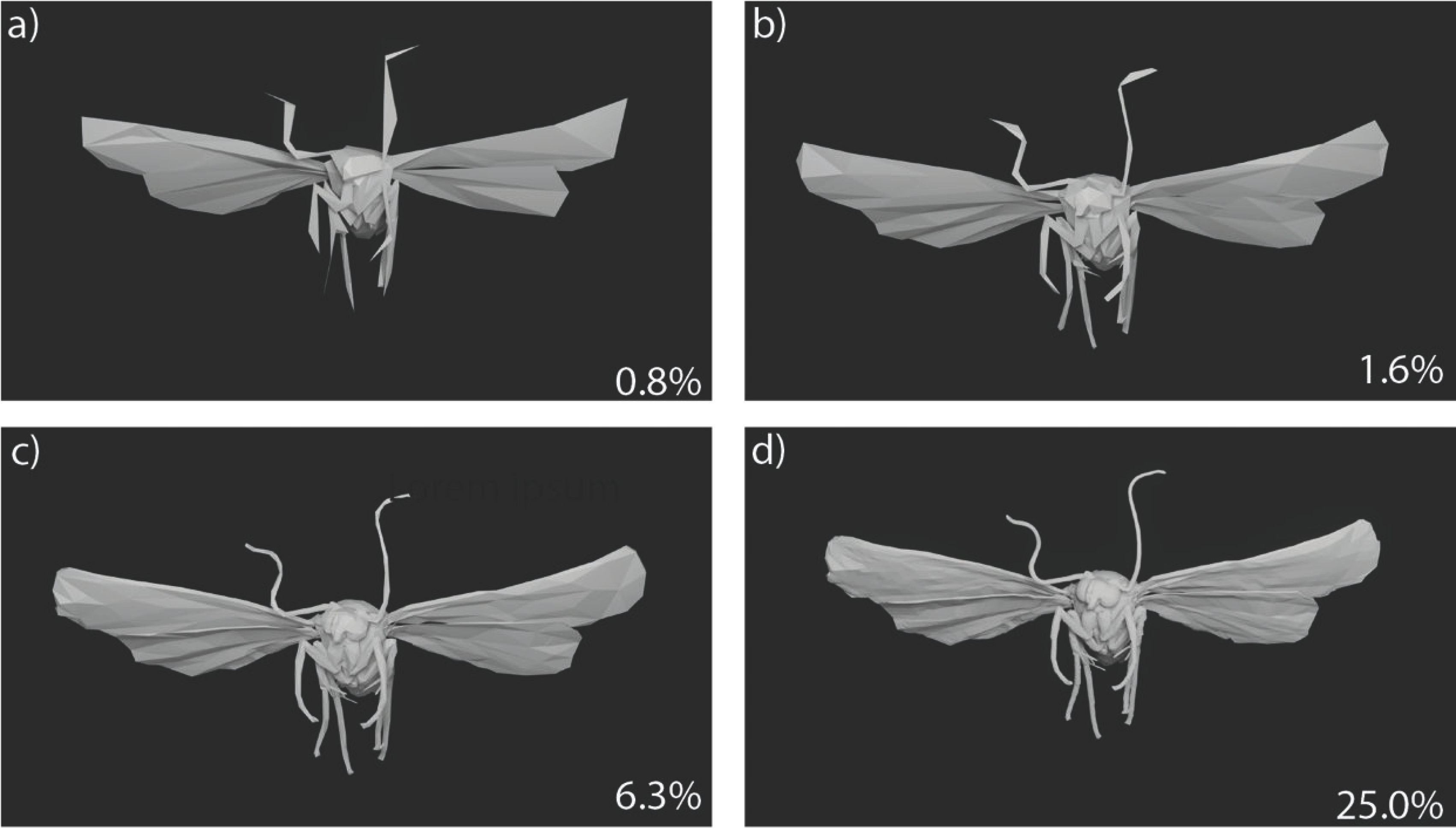
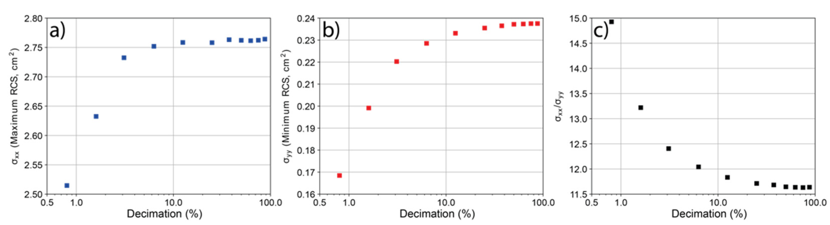
2.5. Model Resolution
2.6. Model Morphology
2.7. Model Composition
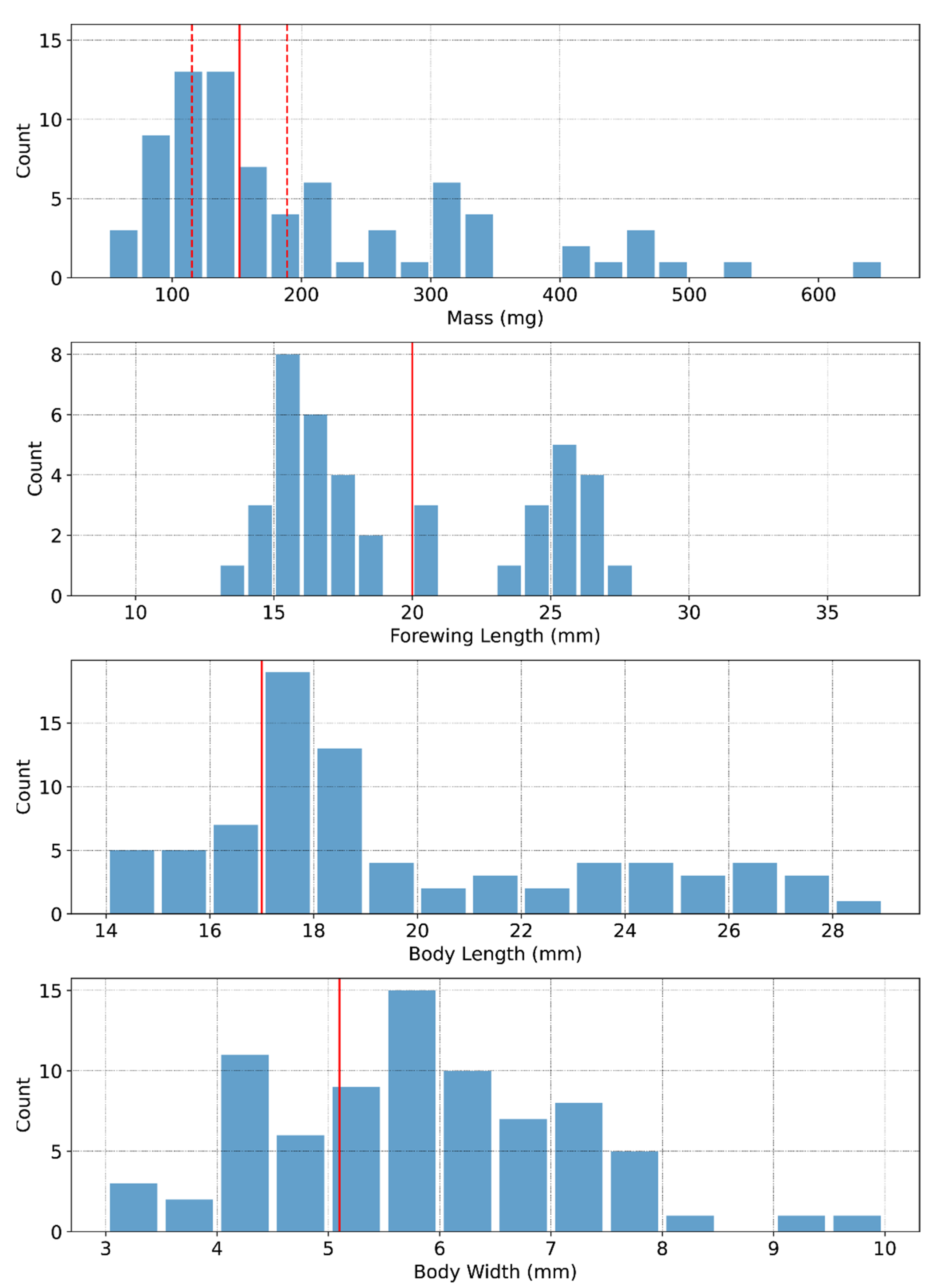
2.8. RCS Reference Dataset
3. Results
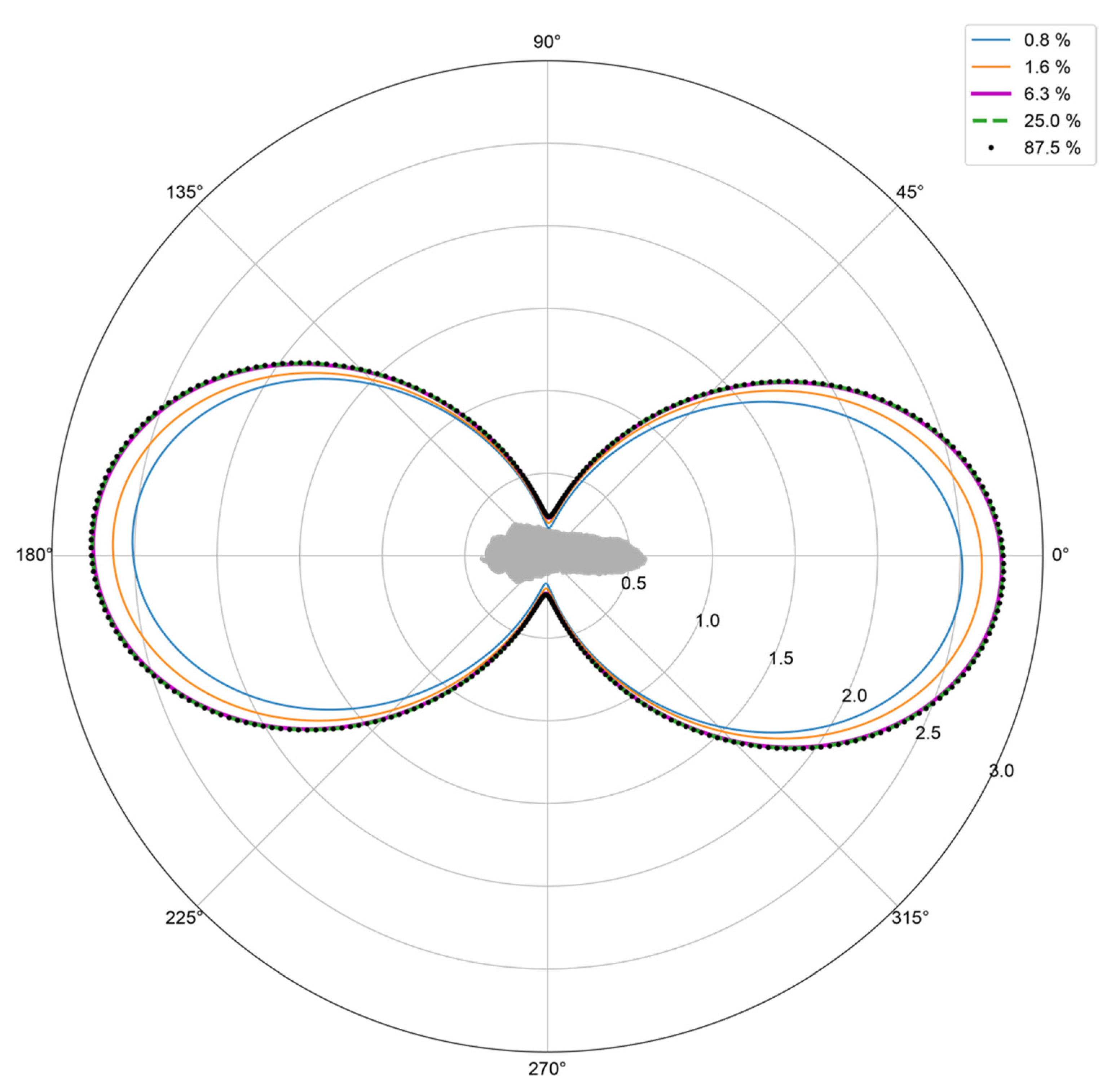
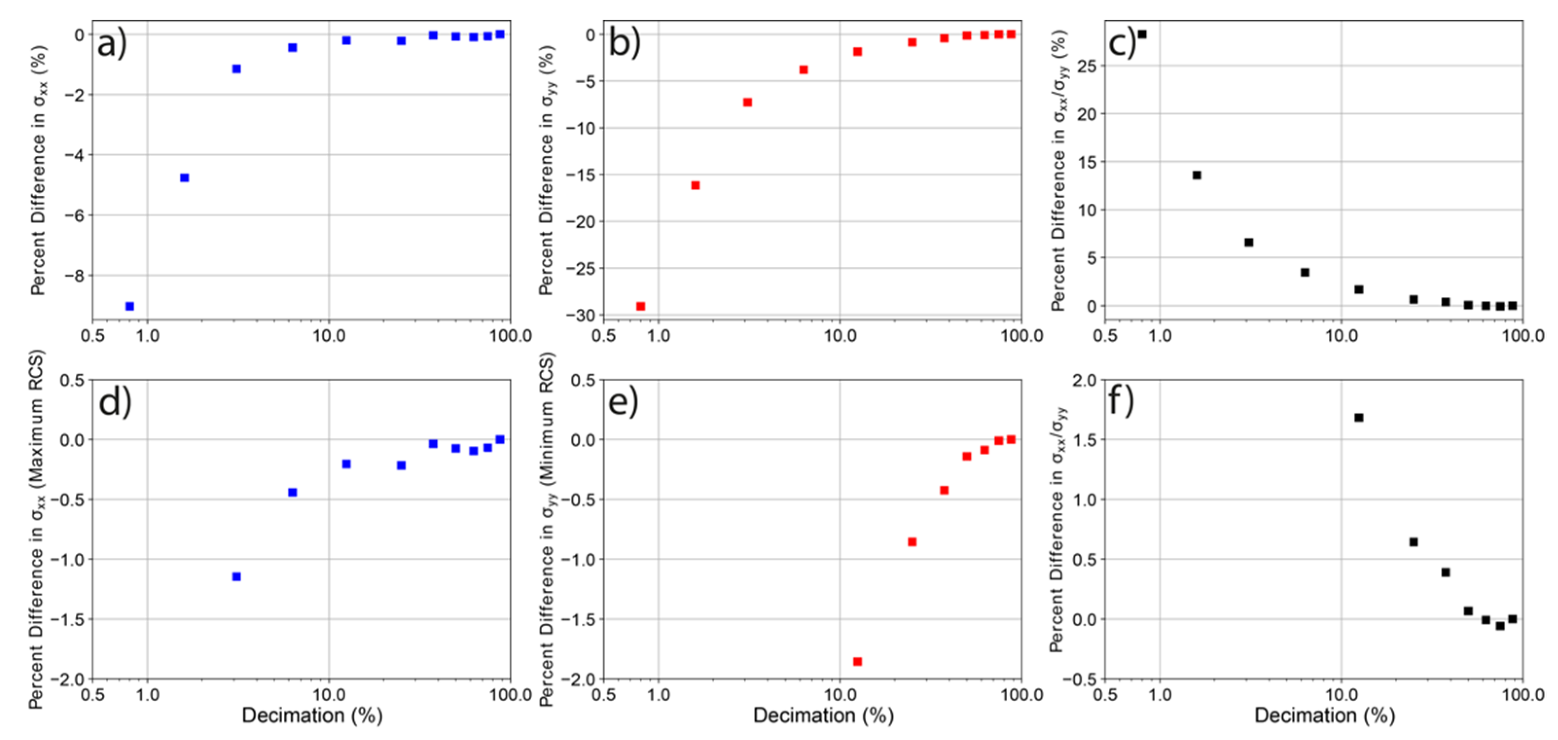
3.1. Model Resolution versus RCS
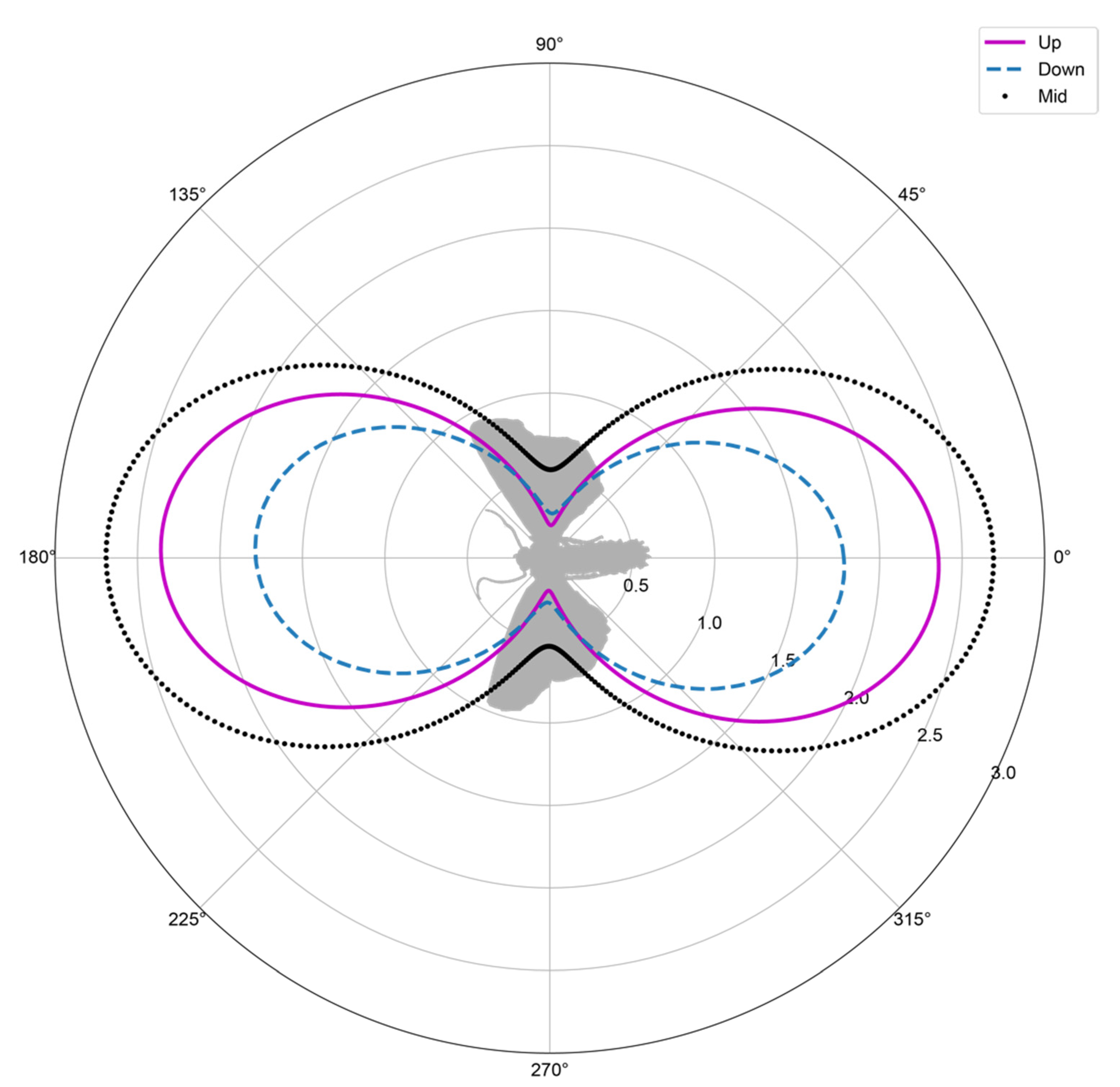
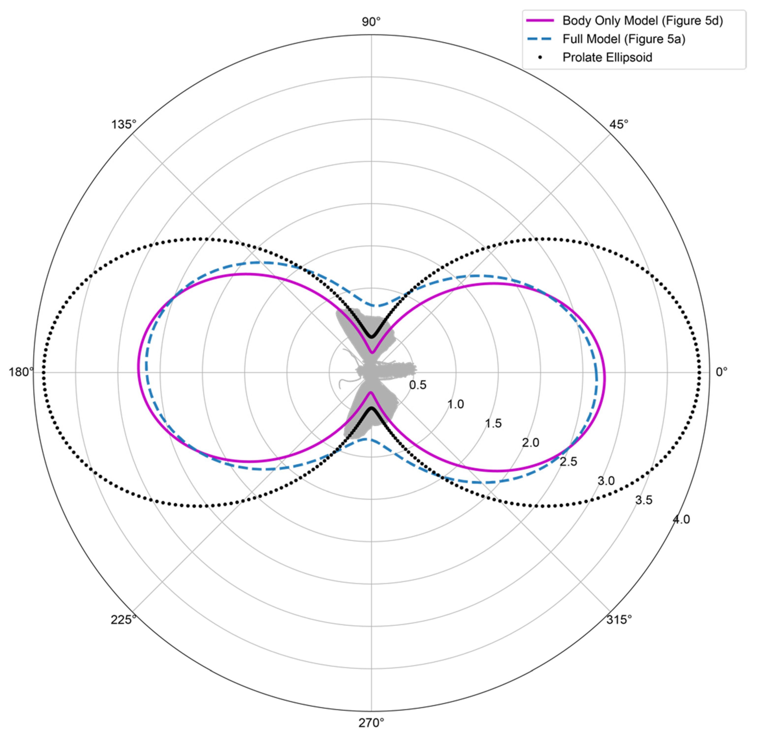
3.2. Model Morphology
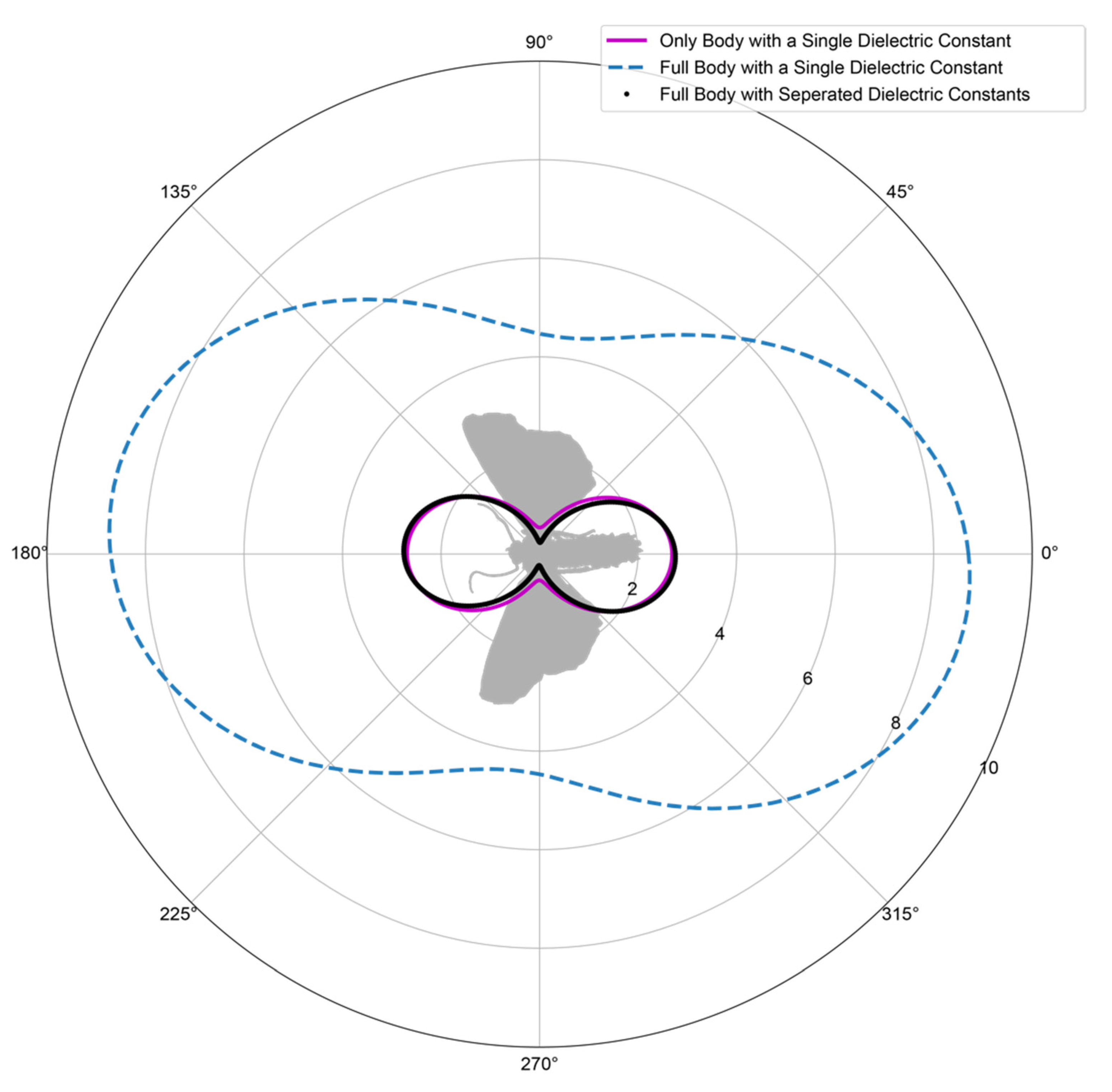
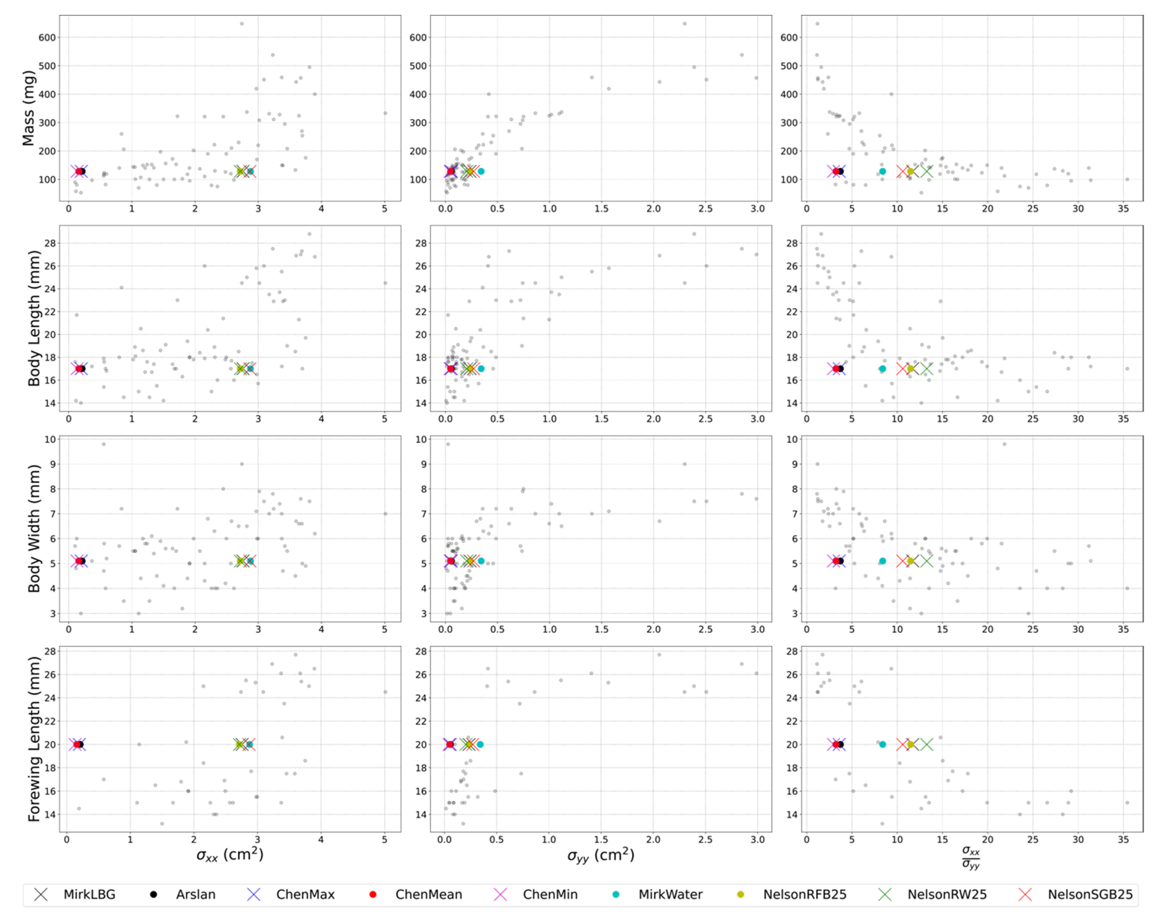
3.3. Composition
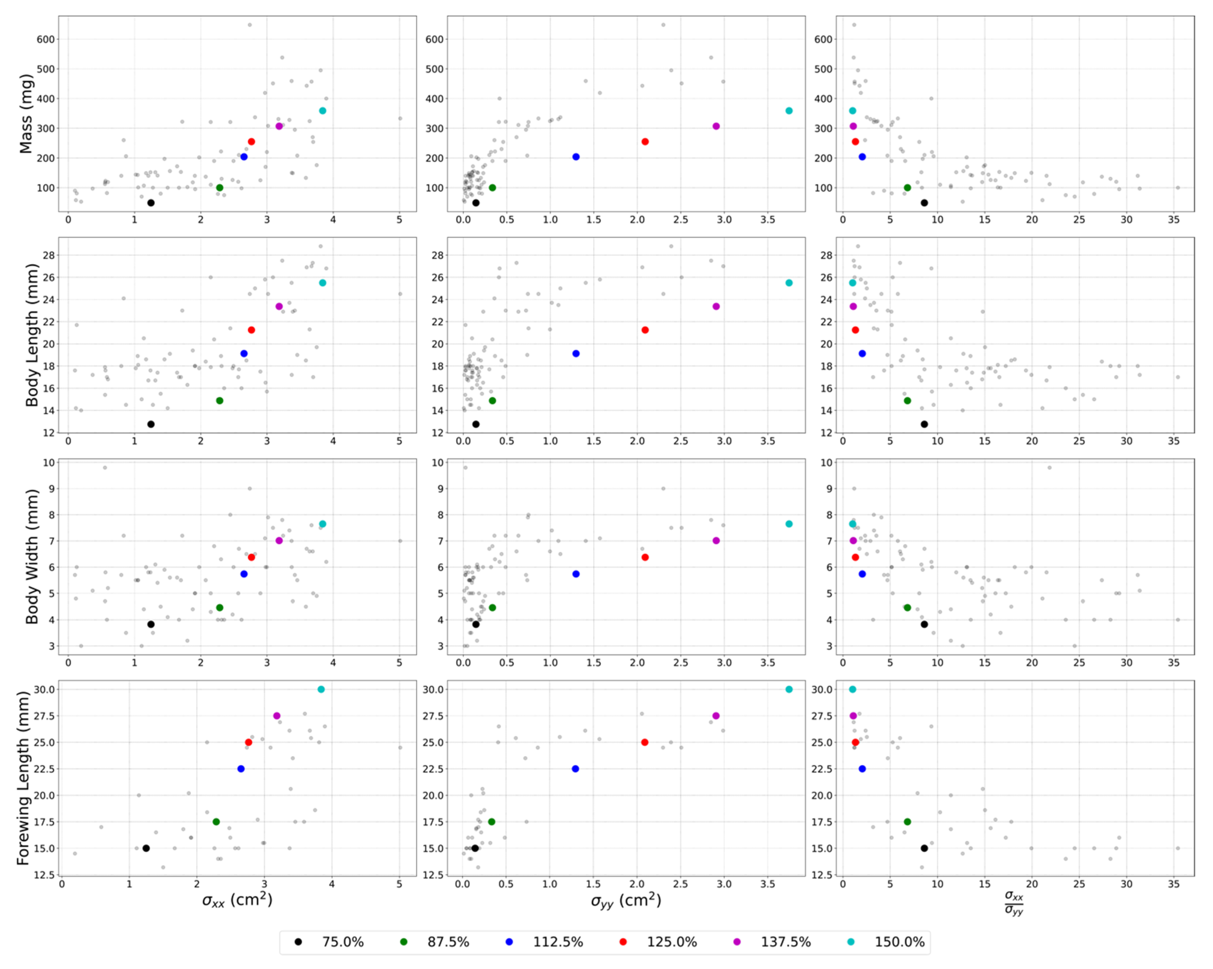
3.4. Scaling
4. Discussion
Author Contributions
Funding
Institutional Review Board Statement
Informed Consent Statement
Data Availability Statement
Acknowledgments
Conflicts of Interest
Appendix A. Molecular Identification of X. xanthographa
Appendix B. Wipl-D Configuration Utilised in All Simulations
- Di3 Files: Off,
- Integral Advanced: Enhanced 1,
- Precision: Double, and
- OM: Monostatic.
Appendix C. Specification of the Computer Resources Used in This Study
References
- Crawford, A.B. Radar Reflections in the Lower Atmosphere. In Proceedings of the IRE; Institute of Radio Engineers IRE: New York, NY, USA, 1949; Volume 37. [Google Scholar]
- Gauthreaux, S.; Belser, C.G. Displays of Bird Movements on the WSR-88D: Patterns and Quantification. Weather Forecast. 1998, 13, 453–464. [Google Scholar] [CrossRef]
- Gauthreaux, S.A.; Livingston, J.W.; Belser, C.G. Detection and discrimination of fauna in the aerosphere using Doppler weather surveillance radar. Integr. Comp. Biol. 2007, 48, 12–23. [Google Scholar] [CrossRef] [PubMed] [Green Version]
- Dokter, A.M.; Liechti, F.; Stark, H.; Delobbe, L.; Tabary, P.; Holleman, I. Bird migration flight altitudes studied by a network of operational weather radars. J. R. Soc. Interface 2011, 8, 30–43. [Google Scholar] [CrossRef] [PubMed] [Green Version]
- Chilson, P.B.; Bridge, E.; Frick, W.F.; Chapman, J.; Kelly, J. Radar aeroecology: Exploring the movements of aerial fauna through radio-wave remote sensing. Biol. Lett. 2012, 8, 698–701. [Google Scholar] [CrossRef] [PubMed]
- Chilson, P.B.; Frick, W.F.; Kelly, J.F.; Howard, K.W.; Larkin, R.P.; Diehl, R.H.; Westbrook, J.K.; Kelly, T.A.; Kunz, T.H. Partly Cloudy with a Chance of Migration: Weather, Radars, and Aeroecology. Bull. Am. Meteorol. Soc. 2012, 93, 669–686. [Google Scholar] [CrossRef]
- Drake, A.; Reynolds, D.R. Radar Entomology: Observing Insect Flight and Migration; CABI: Wallingford, UK, 2012; Available online: https://www.cabi.org/bookshop/book/9781845935566 (accessed on 3 October 2020).
- Stepanian, P.M.; Horton, K.G.; Melnikov, V.M.; Zrnić, D.S.; Gauthreaux, S.A., Jr. Dual-polarization radar products for biological applications. Ecosphere 2016, 7, e01539. [Google Scholar] [CrossRef]
- Mirkovic, D.; Stepanian, P.M.; Wainwright, C.E.; Reynolds, D.R.; Menz, M.H.M. Characterizing animal anatomy and internal composition for electromagnetic modelling in radar entomology. Remote Sens. Ecol. Conserv. 2019, 5, 169–179. [Google Scholar] [CrossRef]
- Stepanian, P.M.; Entrekin, S.A.; Wainwright, C.E.; Mirkovic, D.; Tank, J.L.; Kelly, J.F. Declines in an abundant aquatic insect, the burrowing mayfly, across major North American waterways. Proc. Natl. Acad. Sci. USA 2020, 117, 2987–2992. [Google Scholar] [CrossRef]
- Bauer, S.; Chapman, J.W.; Reynolds, D.R.; Alves, J.; Dokter, A.M.; Menz, M.; Sapir, N.; Ciach, M.; Pettersson, L.B.; Kelly, J.F.; et al. From Agricultural Benefits to Aviation Safety: Realizing the Potential of Continent-Wide Radar Networks. BioScience 2017, 67, 912–918. [Google Scholar] [CrossRef]
- Bauer, S.; Shamoun-Baranes, J.; Nilsson, C.; Farnsworth, A.; Kelly, J.F.; Reynolds, D.R.; Dokter, A.M.; Krauel, J.F.; Petterson, L.B.; Horton, K.G.; et al. The grand challenges of migration ecology that radar aeroecology can help answer. Ecography 2019, 42, 861–875. [Google Scholar] [CrossRef] [Green Version]
- Shamoun-Baranes, J.; Nilsson, C.; Bauer, S.; Chapman, J. Taking radar aeroecology into the 21st century. Ecography 2019, 42, 847–851. [Google Scholar] [CrossRef]
- Shamoun-Baranes, J.; Alves, J.; Bauer, S.; Dokter, A.M.; Hüppop, O.; Koistinen, J.; Leijnse, H.; Liechti, F.; Van Gasteren, H.; Chapman, J.W. Continental-scale radar monitoring of the aerial movements of animals. Mov. Ecol. 2014, 2, 9. [Google Scholar] [CrossRef] [Green Version]
- Melnikov, V.M.; Istok, M.J.; Westbrook, J.K. Asymmetric Radar Echo Patterns from Insects. J. Atmos. Ocean. Technol. 2015, 32, 659–674. [Google Scholar] [CrossRef]
- Mirkovic, D.; Stepanian, P.M.; Kelly, J.F.; Chilson, P.B. Electromagnetic Model Reliably Predicts Radar Scattering Characteristics of Airborne Organisms. Sci. Rep. 2016, 6, 35637. [Google Scholar] [CrossRef] [PubMed]
- Knott, E.F.; Shaeffer, J.F.; Tuley, M.T. Radar Cross Section, 2nd ed.; SciTech Publishing, Inc.: Raleigh, NC, USA, 2004. [Google Scholar]
- Knott, E.F. Radar Cross Section Measurements; Van Nostrand Reinhold: New York, NY, USA, 2012. [Google Scholar]
- Drake, V.A.; Chapman, J.W.; Lim, K.S.; Reynolds, D.R.; Riley, J.R.; Smith, A.D. Ventral-aspect radar cross sections and polarization patterns of insects at X band and their relation to size and form. Int. J. Remote Sens. 2017, 38, 5022–5044. [Google Scholar] [CrossRef]
- Bakker, F.T.; Antonelli, A.; Clarke, J.A.; Cook, J.A.; Edwards, S.V.; Ericson, P.G.; Faurby, S.; Ferrand, N.; Gelang, M.; Gillespie, R.G.; et al. The Global Museum: Natural history collections and the future of evolutionary science and public education. PeerJ 2020, 8, e8225. [Google Scholar] [CrossRef]
- Hedrick, B.P.; Heberling, J.M.; Meineke, E.K.; Turner, K.G.; Grassa, C.J.; Park, D.S.; Kennedy, J.; Clarke, J.; Cook, J.; Blackburn, D.C.; et al. Digitization and the Future of Natural History Collections. BioScience 2020, 70, 243–251. [Google Scholar] [CrossRef]
- Balke, M.; Schmidt, S.; Hausmann, A.; Toussaint, E.F.; Bergsten, J.; Buffington, M.; Häuser, C.L.; Kroupa, A.; Hagedorn, G.; Riedel, A.; et al. Biodiversity into your hands—A call for a virtual global natural history ‘metacollection’. Front. Zool. 2013, 10, 55. [Google Scholar] [CrossRef] [Green Version]
- Waring, P.; Townsend, M. Field Guide to the Moths of Great Britain and Ireland, 3rd ed.; Bloomsbury: London, UK, 2017. [Google Scholar]
- Feng, H.; Wu, X.; Wu, B.; Wu, K. Seasonal Migration of Helicoverpa armigera (Lepidoptera: Noctuidae) Over the Bohai Sea. J. Econ. Entomol. 2009, 102, 95–104. [Google Scholar] [CrossRef]
- Feng, H.Q.; Zhao, X.C.; Wu, X.F.; Wu, B.; Wu, K.M.; Cheng, D.F.; Guo, Y.Y. Autumn Migration of Mythimna Separata (Lepidoptera: Noctuidae) over the Bohai Sea in Northern China. Environ. Entomol. 2008, 37, 774–781. [Google Scholar] [CrossRef]
- Westbrook, J.K. Noctuid migration in Texas within the nocturnal aeroecological boundary layer. Integr. Comp. Biol. 2008, 48, 99–106. [Google Scholar] [CrossRef] [PubMed] [Green Version]
- Li, C.; Fu, X.; Feng, H.; Ali, A.; Li, C.; Wu, K. Seasonal Migration of Ctenoplusia agnata (Lepidoptera: Noctuidae) Over the Bohai Sea in Northern China. J. Econ. Entomol. 2014, 107, 1003–1008. [Google Scholar] [CrossRef] [PubMed]
- Fu, X.; Feng, H.; Liu, Z.; Wu, K. Trans-regional migration of the beet armyworm, Spodoptera exigua (Lepidoptera: Noctuidae), in North-East Asia. PLoS ONE 2017, 12, e0183582. [Google Scholar] [CrossRef] [PubMed] [Green Version]
- Westbrook, J.; Eyster, R. Doppler weather radar detects emigratory flights of noctuids during a major pest outbreak. Remote Sens. Appl. Soc. Environ. 2017, 8, 64–70. [Google Scholar] [CrossRef]
- Fu, X.; Zhao, X.; Xie, B.; Ali, A.; Wu, K. Seasonal Pattern of Spodoptera litura (Lepidoptera: Noctuidae) Migration across the Bohai Strait in Northern China. J. Econ. Entomol. 2015, 108, 525–538. [Google Scholar] [CrossRef] [PubMed]
- Wood, C.; Reynolds, D.; Wells, P.; Barlow, J.; Woiwod, I.; Chapman, J. Flight periodicity and the vertical distribution of high-altitude moth migration over southern Britain. Bull. Entomol. Res. 2009, 99, 525–535. [Google Scholar] [CrossRef] [Green Version]
- Wood, C.R.; Chapman, J.W.; Reynolds, D.R.; Barlow, J.F.; Smith, A.D.; Woiwod, I.P. The influence of the atmospheric boundary layer on nocturnal layers of noctuids and other moths migrating over southern Britain. Int. J. Biometeorol. 2006, 50, 193–204. [Google Scholar] [CrossRef]
- Chapman, J.W.; Lim, K.S.; Reynolds, D.R. The significance of midsummer movements of Autographa gamma: Implications for a mechanistic understanding of orientation behavior in a migrant moth. Curr. Zool. 2013, 59, 360–370. [Google Scholar] [CrossRef] [Green Version]
- Chapman, J.W.; Reynolds, D.; Mouritsen, H.; Hill, J.K.; Riley, J.R.; Sivell, D.; Smith, A.D.; Woiwod, I.P. Wind Selection and Drift Compensation Optimize Migratory Pathways in a High-Flying Moth. Curr. Biol. 2008, 18, 514–518. [Google Scholar] [CrossRef] [Green Version]
- NBN Atlas. Available online: https://species.nbnatlas.org/species/NHMSYS0021144939#overview (accessed on 3 October 2020).
- Fedorov, A.; Beichel, R.; Kalpathy-Cramer, J.; Finet, J.; Fillion-Robin, J.-C.; Pujol, S.; Bauer, C.; Jennings, D.; Fennessy, F.; Sonka, M.; et al. 3D Slicer as an image computing platform for the Quantitative Imaging Network. Magn. Reson. Imaging 2012, 30, 1323–1341. [Google Scholar] [CrossRef] [Green Version]
- Blender Online Community. Blender—A 3D Modelling and Rendering Package; Stichting Blender Foundation: Amsterdam, The Netherlands, 2018. [Google Scholar]
- Denning, J.; Lampel, J.; Williamson, J.; Moore, P.; Crawford, P.; Gearhart, C. Retopoflow: A Suite of Retopology Tools for Blender through a Unified Retopology Mode. Version 3.0, Beta 2. 2020. Available online: https://github.com/CGCookie/retopoflow (accessed on 3 October 2020).
- Wasserthal, L.T. Respiratory System. In Handbook of Zoology: Lepidoptera, Moths and Butterflies; Kristensen, N.P., Ed.; De Gruyter: Berlin, Germany, 2003; Volume 4/36-2, pp. 189–203. [Google Scholar]
- Simelane, S.M.; Abelman, S.; Duncan, F.D. Gas Exchange Models for a Flexible Insect Tracheal System. Acta Biotheor. 2016, 64, 161–196. [Google Scholar] [CrossRef] [PubMed]
- Kolundzija, B.M. Electromagnetic modeling of composite metallic and dielectric structures. IEEE Trans. Microw. Theory Tech. 1999, 47, 1021–1032. [Google Scholar] [CrossRef]
- Kolundzija, B.; Ognjanovic, J.; Sarkar, T.; Harrington, R. WIPL: A program for electromagnetic modeling of composite-wire and plate structures. IEEE Antennas Propag. Mag. 1996, 38, 75–79. [Google Scholar] [CrossRef]
- Smith, A.; Reynolds, D.; Riley, J. The use of vertical-looking radar to continuously monitor the insect fauna flying at altitude over southern England. Bull. Entomol. Res. 2000, 90, 265–277. [Google Scholar] [CrossRef] [PubMed]
- Drake, V. Signal processing for ZLC-configuration insect-monitoring radars: Yields and sample biases. In Proceedings of the International Conference on Radar IEEE, Adelaide, Australia, 9–12 September 2013; pp. 298–303. [Google Scholar] [CrossRef]
- Drake, V.A. Distinguishing target classes in observations from vertically pointing entomological radars. Int. J. Remote Sens. 2016, 37, 3811–3835. [Google Scholar] [CrossRef]
- Nelson, S.O.; Bartley, P.G., Jr.; Lawrence, K.C. RF and microwave dielectric properties of stored-grain insects and their implications for potential insect control. Trans. ASAE 1998, 41, 685–692. [Google Scholar] [CrossRef]
- Dorsett, D.A. Preparation for Flight by Hawk-Moths. J. Exp. Biol. 1962, 39, 579–588. [Google Scholar] [CrossRef]
- Heath, J.E.; Adams, P.A. Regulation of Heat Production by Large Moths. J. Exp. Biol. 1967, 47, 21–33. [Google Scholar] [CrossRef]
- Bartholomew, G.A.; Heinrich, B. A Field Study of Flight Temperatures in Moths in Relation to Body Weight and Wing Loading. J. Exp. Biol. 1973, 58, 123–135. [Google Scholar] [CrossRef]
- Chen, H.; Li, X.; Yu, W.; Wang, J.; Shi, Z.; Xiong, C.; Yang, Q. Chitin/MoS2 Nanosheet Dielectric Composite Films with Significantly Enhanced Discharge Energy Density and Efficiency. Biomacromolecules 2020, 21, 2929–2937. [Google Scholar] [CrossRef]
- Chapman, J.; Reynolds, D.; Smith, A.; Smith, E.; Woiwod, I. An aerial netting study of insects migrating at high altitude over England. Bull. Entomol. Res. 2004, 94, 123–136. [Google Scholar] [CrossRef]
- Sane, S.P. The aerodynamics of insect flight. J. Exp. Biol. 2003, 206, 4191–4208. [Google Scholar] [CrossRef] [PubMed] [Green Version]
- Aiello, B.R.; Bin Sikandar, U.; Minoguchi, H.; Bhinderwala, B.; Hamilton, C.A.; Kawahara, A.Y.; Sponberg, S. The evolution of two distinct strategies of moth flight. J. R. Soc. Interface 2021, 18, 20210632. [Google Scholar] [CrossRef] [PubMed]
- Andryieuski, A.; Kuznetsova, S.M.; Zhukovsky, S.V.; Kivshar, Y.S.; Lavrinenko, A.V. Water: Promising Opportunities for Tunable All-dielectric Electromagnetic Metamaterials. Sci. Rep. 2015, 5, 13535. [Google Scholar] [CrossRef] [Green Version]
- Kong, S.; Hu, C.; Wang, R.; Zhang, F.; Wang, L.; Long, T.; Wu, K. Insect Multifrequency Polarimetric Radar Cross Section: Experimental Results and Analysis. IEEE Trans. Geosci. Remote Sens. 2021, 59, 6573–6585. [Google Scholar] [CrossRef]
- Truett, G.; Heeger, P.; Mynatt, R.; Truett, A.; Walker, J.; Warman, M. Preparation of PCR-Quality Mouse Genomic DNA with Hot Sodium Hydroxide and Tris (HotSHOT). BioTechniques 2000, 29, 52–54. [Google Scholar] [CrossRef] [PubMed]
- Folmer, O.; Black, M.; Hoeh, W.; Lutz, R.; Vrijenhoek, R. DNA primers for amplification of mitochondrial cytochrome c oxidase subunit I from diverse metazoan invertebrates. Mol. Mar. Biol. Biotechnol. 1994, 3, 294–299. [Google Scholar]
- Hajibabaei, M.; Janzen, D.H.; Burns, J.M.; Hallwachs, W.; Hebert, P.D.N. DNA barcodes distinguish species of tropical Lepidoptera. Proc. Natl. Acad. Sci. USA 2006, 103, 968–971. [Google Scholar] [CrossRef] [Green Version]


| Material | Description | Dielectric Constant | Loss Factor | Abbrev. | Density (g/cm3) | Source | Notes |
|---|---|---|---|---|---|---|---|
| Homogenised blend of the lesser grain borer beetle | Insect paste utilised by Mirkovic et al. [9] for the lesser grain boorer, Rhyzopertha dominica. Temperature unspecified. | 34.3 | −18.6 | MirkLGB | 1.26 | [9,46] | Used to compare the simulations of this study to Mirkovic et al. [9]. Values are taken directly from Nelson et al. [46] as part of the four species examined therein. |
| Homogenised blend of the rice weevil | Insect paste of the rice weevil, Sitophilus oryzae, at 25 °C. | 30.6 | −16 | NelsonRW25 | 1.29 | [46] | |
| Homogenised blend of the red flour beetle | Insect paste of the red flour beetle, Tribolium castaneum, at 25 °C. | 34.0 | −19.4 | NelsonRFB25 | 1.29 | [46] | |
| Homogenised blend of the saw-toothed grain beetle | Insect paste of the sawtoothed grain beetle, Oryzaephilus surinamensis, at 25 °C. | 39.8 | −20.8 | NelsonSGB25 | 1.34 | [46] | |
| Chitin | Chitin film at room temperature. | 4.1 | −0.16 | ChenMean | [50] | Extrapolated to 9.4 GHz. Values are the mean of this estimation. | |
| Chitin | Chitin film at room temperature. | 4.5 | −0.18 | ChenMax | [50] | Extrapolated to 9.4 GHz. Values are the maximum of this estimation. | |
| Chitin | Chitin film at room temperature. | 3.8 | −0.14 | ChenMin | [50] | Extrapolated to 9.4 GHz. Values are the minimum of this estimation. | |
| Water | Water used in Mirkovic et al. [9]. Temperature unspecified. | 60.3 | −33.1 | MirkWater | 1.00 | [9] | Used to compare the simulations of this study to Mirkovic et al. [9]. |
Publisher’s Note: MDPI stays neutral with regard to jurisdictional claims in published maps and institutional affiliations. |
© 2022 by the authors. Licensee MDPI, Basel, Switzerland. This article is an open access article distributed under the terms and conditions of the Creative Commons Attribution (CC BY) license (https://creativecommons.org/licenses/by/4.0/).
Share and Cite
Addison, F.I.; Dally, T.; Duncan, E.J.; Rouse, J.; Evans, W.L.; Hassall, C.; Neely, R.R., III. Simulation of the Radar Cross Section of a Noctuid Moth. Remote Sens. 2022, 14, 1494. https://doi.org/10.3390/rs14061494
Addison FI, Dally T, Duncan EJ, Rouse J, Evans WL, Hassall C, Neely RR III. Simulation of the Radar Cross Section of a Noctuid Moth. Remote Sensing. 2022; 14(6):1494. https://doi.org/10.3390/rs14061494
Chicago/Turabian StyleAddison, Freya I., Thomas Dally, Elizabeth J. Duncan, James Rouse, William L. Evans, Christopher Hassall, and Ryan R. Neely, III. 2022. "Simulation of the Radar Cross Section of a Noctuid Moth" Remote Sensing 14, no. 6: 1494. https://doi.org/10.3390/rs14061494
APA StyleAddison, F. I., Dally, T., Duncan, E. J., Rouse, J., Evans, W. L., Hassall, C., & Neely, R. R., III. (2022). Simulation of the Radar Cross Section of a Noctuid Moth. Remote Sensing, 14(6), 1494. https://doi.org/10.3390/rs14061494