Automated Delineation of Microstands in Hemiboreal Mixed Forests Using Stereo GeoEye-1 Data

Abstract

A microstand is a small forest area with a homogeneous tree species, height, and density composition. High-spatial-resolution GeoEye-1 multispectral (MS) images and GeoEye-1-based canopy height models (CHMs) allow delineating microstands automatically. This paper studied the potential benefits of two microstand segmentation workflows: (1) our modification of JSEG and (2) generic region merging (GRM) of the Orfeo Toolbox, both intended for the microstand border refinement and automated stand volume estimation in hemiboreal forests. Our modification of JSEG uses a CHM as the primary data source for segmentation by refining the results using MS data. Meanwhile, the CHM and multispectral data fusion were achieved as multiband segmentation for the GRM workflow. The accuracy was evaluated using several sets of metrics (unsupervised, supervised direct assessment, and system-level assessment). Metrics were calculated for a regular segment grid to check the benefits compared with the simple image patches. The metrics showed very similar results for both workflows. The most successful combinations in the workflow parameters retrieved over 75 % of the boundaries selected by a human interpreter. However, the impact of data fusion and parameter combinations on stand volume estimation accuracy was minimal, causing variations of the RMSE within approximately 7 m${}^3$/ha.

1. Introduction

Accurate information about forests’ qualitative and quantitative conditions (forest inventory) is critical to effectively achieving forest management’s economic, environmental, and social goals.

Remote sensing data provide spatially detailed information over vast areas and can be used as a complementary information source for an automated forest inventory [1]. Especially, very-high-resolution (VHR) stereo satellite images may be beneficial by offering up-to-date information about both the spectral and structural characteristics of the forest, since the cycles of updating aerial imagery and LiDAR data throughout the given area are much less frequent. For example, aerial photography of the entire territory of Latvia is carried out every three years, while laser scanning was performed only once [2].

Various processing methods have been applied to support national forest inventories (NFIs) depending on a remote sensing data source [3]. Data processing workflows can be grouped by the employed datasets and by the spatial units in which forest inventory variable estimations are carried out. For example, the spatial unit of an automated forest inventory based on remote sensing data can be: (1) a pixel [4], (2) a single tree [5], and (3) homogeneous image patches or forest microstands [6].

The most accurate forest inventory parameter estimations can be achieved by operating at the single-tree level [7]. However, a successful individual tree identification and delineation greatly depend on the spatial resolution of the remote sensing data and forest conditions (such as the tree species composition and stand density) [8,9]. For example, dense deciduous and mixed stands with a visually flat crown shape in remote sensing data and overlapping tree crowns are frequent in hemiboreal mixed forests. As a result, the detection of a single tree is limited under such conditions even when remote sensing data of a high spatial resolution are available.

Thus, this study focused on microstands as operational units for potentially automated forest inventory data collection. In the sense of remote-sensing-based forest inventory, microstands are homogeneous forest patches [10], which are the same in terms of tree species, height, and composition without restrictions on the minimal allowed area or borders imposed by management aspects. According to the legislation or forest management needs, microstands can be combined into forest compartments.

During the general forest inventory procedure in the Baltic States, a map of forest compartments that unites the stands of similar age, forest type, and height composition is created according to the local legislation [11]. Those compartments serve as a basic spatial unit for summarizing forest inventory variables such as stand volume, stand height, etc. Compartment borders are generally associated with homogeneous forest patches, as well as with management units and historically established compartment borders.

Typically, forest inventory specialists/evaluatorsacquire primary forest inventory parameters and refine compartment borders through field campaigns and remote sensing data visual analysis (aerial images, LiDAR-based canopy height models (CHMs)). The allocation of forest compartments is highly dependent on the experience of each particular forest inventory specialist [12]. In addition, legalisation [11] in Latvia also states that the minimum allowed forest compartment area is 0.3 ha; therefore, smaller forest features are often overlooked.

After collecting in situ data, evaluatorssubmit the data of primary forest inventory indicators, such as species composition, height, and diameter, to the State Forest Register, where secondary inventory indicators are calculated from them, for example stand volume.

Microstands can also be delineated using remote sensing data by image segmentation techniques [13] and can serve as a more robust spatial unit applicable in daily practice to vast areas with complicated structures of forest stands. An example of such an approach is the forest inventory procedure used in Finland, where forest areas are automatically subdivided into irregular larger or smaller microstands according to remote sensing data [6].

Forest compartment and microstand delineation methods using remote sensing data can be classified into two groups: (1) workflows based on segmentation methods and (2) workflows based on the detection of single trees merged into microstands.

Many segmentation-based studies (first group) employ the popular Baatz and Schäpe segmentation algorithm [14] implemented in the eCognition software [15,16,17,18,19]. The algorithm includes the region-growing segmentation by minimizing the spectral and spatial heterogeneity of the segments. Several datasets, including orthophotos [20], LiDAR-based feature images [21], and optical and LiDAR data fusion [15], can be processed using this method. The region-growing approach is also employed in other studies [22,23]. While most methods work with raster images, Bruggisser et al. [24] employed the k-means clustering of the LiDAR point cloud, followed by an iterative merging step to tackle the oversegmentation.

The second approach unites smaller spatial units such as single-tree objects or grid cells into microstands based on the mutual similarity between neighbouring units. Leckie et al. [25] identified single-tree crowns using the valley-following approach, classified the tree species, and formed stands by accounting for stem density and canopy closure. Deschesne et al. [26] combined pixel-level features with the watershed-based single-tree extraction to segment semantic forest classes. Instead of single-tree crowns, Koch et al. [12] analysed grid cells to find uniform data units, while Jia et al. [27] applied cellular automation for stand delineation.

A comparison of different studies to find an optimal dataset, data processing workflow, and its parameters is burdened by the subjectivity factor in microstand borders and a lack of a set of unambiguous metrics allowing selecting the best segmentation result [28]. Wulder et al. [29] stated that an objective accuracy assessment of polygons using the ground truth cannot be achieved in forest stand delineation, because stand borders are not so clear as in the case of urban or agricultural applications. The selection of forest stands by image analysts can differ between experts [12]. The microstand delineation accuracy can be measured using two basic approaches: (1) system-level and (2) direct assessments [28]. The system-level accuracy assessment means evaluating segmentation results in a comprehensive workflow for estimating forest inventory variables. The higher accuracy of those forest inventory variables hints at a more efficient segmentation [23,26]. The direct accuracy assessment includes evaluating the quality of the segments using reference data such as stands delineated by experts (supervised assessment) [21] or segment homogeneity criteria [17] (unsupervised assessment).

The objective of this research was to investigate the application of two microstand segmentation workflows: (1) our modification of JSEG and (2) generic region merging (GRM) of the Orfeo Toolbox, both for the microstand border refinement (to provide additional input for traditional forest inventory process) and automated stand volume estimation in hemiboreal mixed forests.

The main contribution of this research is related to the performance analysis of the microstand segmentation algorithms in the case of highly heterogeneous hemiboreal forest stands.

Our contribution in this research also includes:

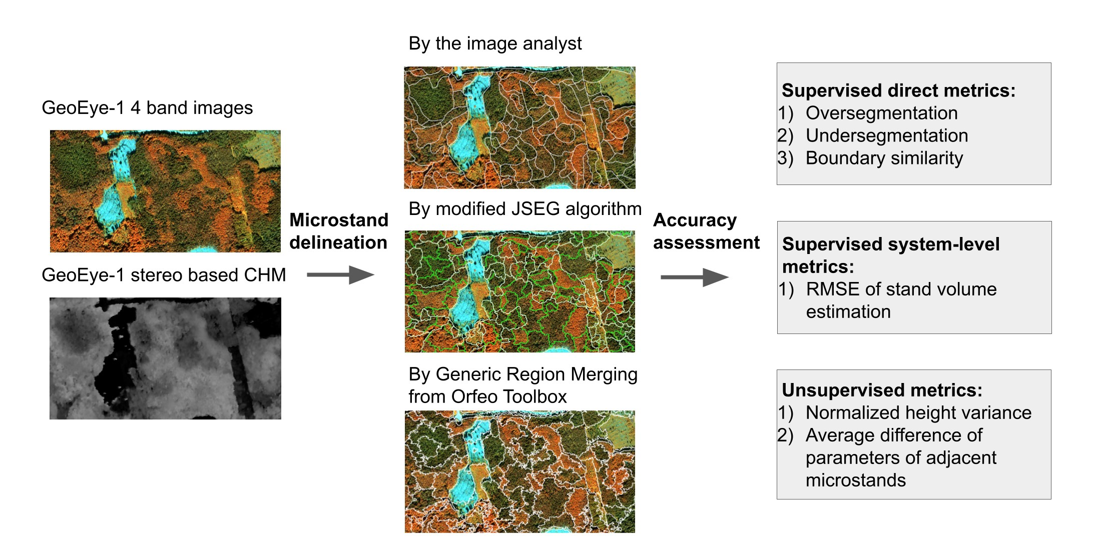
• Development of modified JSEG segmentation [30] workflow in a way providing for the CHM and multispectral data fusion;
• Application of the JSEG workflow and freeware solution provided by the Orfeo Toolbox: Generic Region Merging to four-band GeoEye-1 images and the CHM prepared using the same GeoEye-1 stereo scene. The CHM produced in this manner includes time compatibility with the spectral bands;
• Extensive accuracy assessment for hemiboreal forests in Latvia using (1) unsupervised and forest-specific metrics, (2) supervised, direct accuracy assessment using 2700 microstands delineated by an independent image analyst, and (3) system-level assessment by estimating stand volume. All metrics were also calculated for grid cells to evaluate the benefits of segmentation.

Hemiboreal forests are characterised by the dominance of coniferous trees, but with a significant presence of numerous deciduous tree species [31], resulting in high spectral and structural variability within a stand and between stands. This diversity poses challenges for both segmentation and machine learning algorithms.

The motivation for choosing JSEG [30] for this study was the ability of the algorithm to capture uniform, high-level textures, which are specifically important for the delineation of microstands. Texture created by tree crowns is one of the most important features observed by image analysts when selecting microstands by hand. The JSEG segmentation method has been proven efficient for extracting regions of similar texture without restrictions on the region size [30]. Wang et al. [32] compared the classical and improved JSEG method with the eCognition segmentation algorithm and concluded that improved JSEG could retrieve boundaries better. However, comparatively, JSEG has been considered in a small amount of studies. This could be the lack of open-source implementations and the high computational complexity.

The generic region merging of Orfeo Toolbox (OTB) was chosen for comparison because it is a freely available and easy-to-use implementation.

2. Materials and Methods

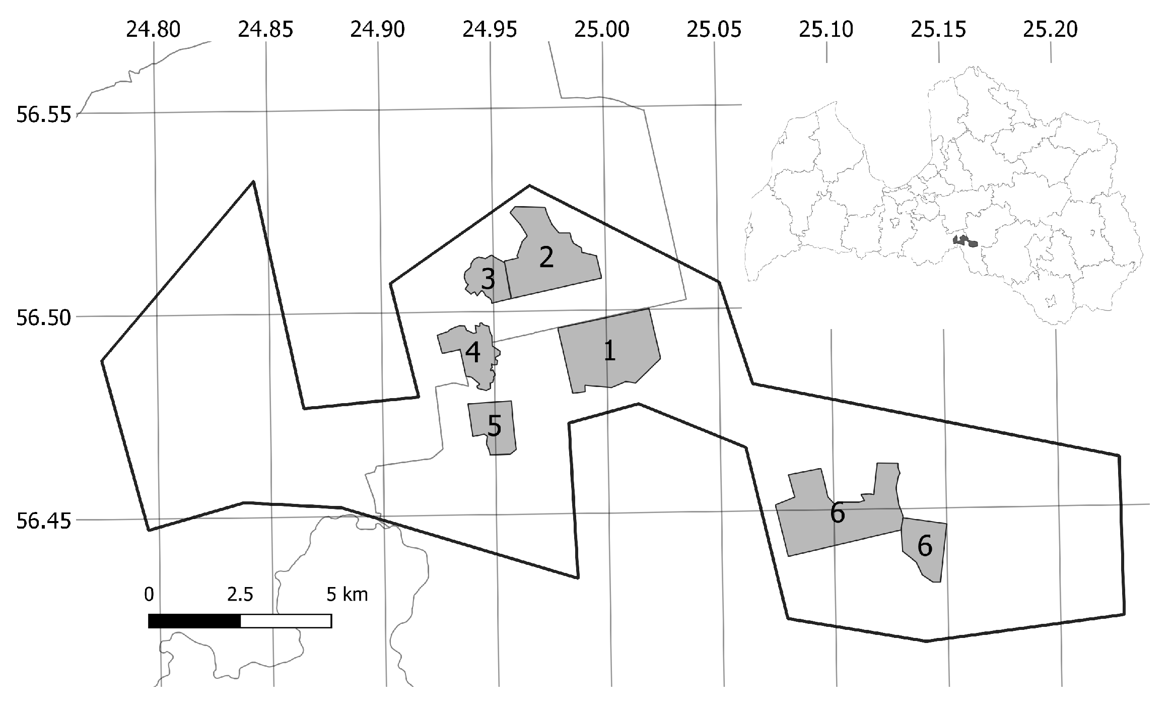
2.1. Study Site

Microstand segmentation was performed for an approximately 161 km${}^2$ large area in the central-southern part of Latvia (56.46${}^{°}$N, 25.04${}^{°}$E) near the Lithuanian border; see Figure 1. The study area includes hemiboreal mixed forest, in which the dominant tree species are Scots pine (Pinus sylvestris L.), Norway spruce (Picea abies (L.) Karst.), birch (Betula pendula Roth and Betula pubescens Ehrh.), and black alder (Alnus glutinosa (L.) Gaertn).

More than half of the area is owned by the Joint Stock Company “Latvia’s State Forests” (LVM), but the rest is occupied by forests of private owners and non-forested land cover types. The average stand age of the state-owned forests is 66 y, with a standard deviation of 34 y, according to the National Forest Inventory (NFI) database. State-owned forest stands are under heavier management activities than private owners, resulting in visibly different textures formed by tree crowns in the VHR images.

Microstand polygon reference data were acquired during this research for six sample areas (for both state and private lands within the study site) with a total area of 19.5 km${}^2$.

2.2. Remote Sensing and Reference Data

We used GeoEye-1 stereo image pairs acquired at 9:27 on 7 August 2020. Each scene includes 4-band (blue: 450–510 nm, green: 510–580 nm, red: 655–690 nm, and near-infrared: 780–920 nm) multispectral data with a spatial resolution of 2m/px and the panchromatic band (450–800 nm) with a 0.5 m/px resolution [33].

The canopy height model (CHM) was prepared on a 0.5 m/px grid employing the PCI Geomatica software, by using near-infrared stereo images from the same GeoEye-1 scene and the external digital terrain model (DTM) provided by the Latvian Geospatial Information Agency.

Microstand segmentation was performed using only GeoEye-1 MS and CHM data. For validation purposes, we also employed LiDAR-based CHM with a spatial resolution of 0.5 m/px, which allowed us to evaluate the approximate number of tree crowns within a microstand.

The reference dataset included the NFI database for state forests within a study site and 2770 microstand polygons drawn by the image analyst for 6 sample areas.

The image analyst (researcher in the field of forestry, hired for this research) visually assessed the remote sensing datasets mentioned above by analysing the CHM first and using multispectral information to split polygons found in the CHM if necessary. For every polygon, the image analyst assigned 1 of 5 land cover class codes (1—pure stand containing only 1 tree species, 2—mixed stand containing more than 1 tree species, 3—recently felled area, 4—non-forest, 5—young stand) and the confidence level of microstand border position. If the microstand border was clearly visible in the remote sensing data as in case of even-aged pure stands, then the expert recorded a confidence level of 1 (high confidence). If the borders selected might be ambiguous or hard to distinguish, then the confidence level of 0 (low confidence) was assigned. A summary of the spatial characteristics for the six sample areas is given in

Table 1. Characteristics of the sample areas derived from the reference data.

No.	Area (km${}^2$)	Number of Microstands	Percentage of the Forested Area Owned by the State	Percentage of the Area Formed by Mixed Stands	Percentage of the Area Delineated with Low Confidence
1	4.54	508	46	51.4	12.8
2	3.85	545	62	42.8	31.5
3	1.16	194	7	45.2	15.6
4	1.67	336	88	53.1	40.4
5	1.44	208	18	33.5	34.3
6	6.83	979	73	40.6	13.8

.

2.3. Methods

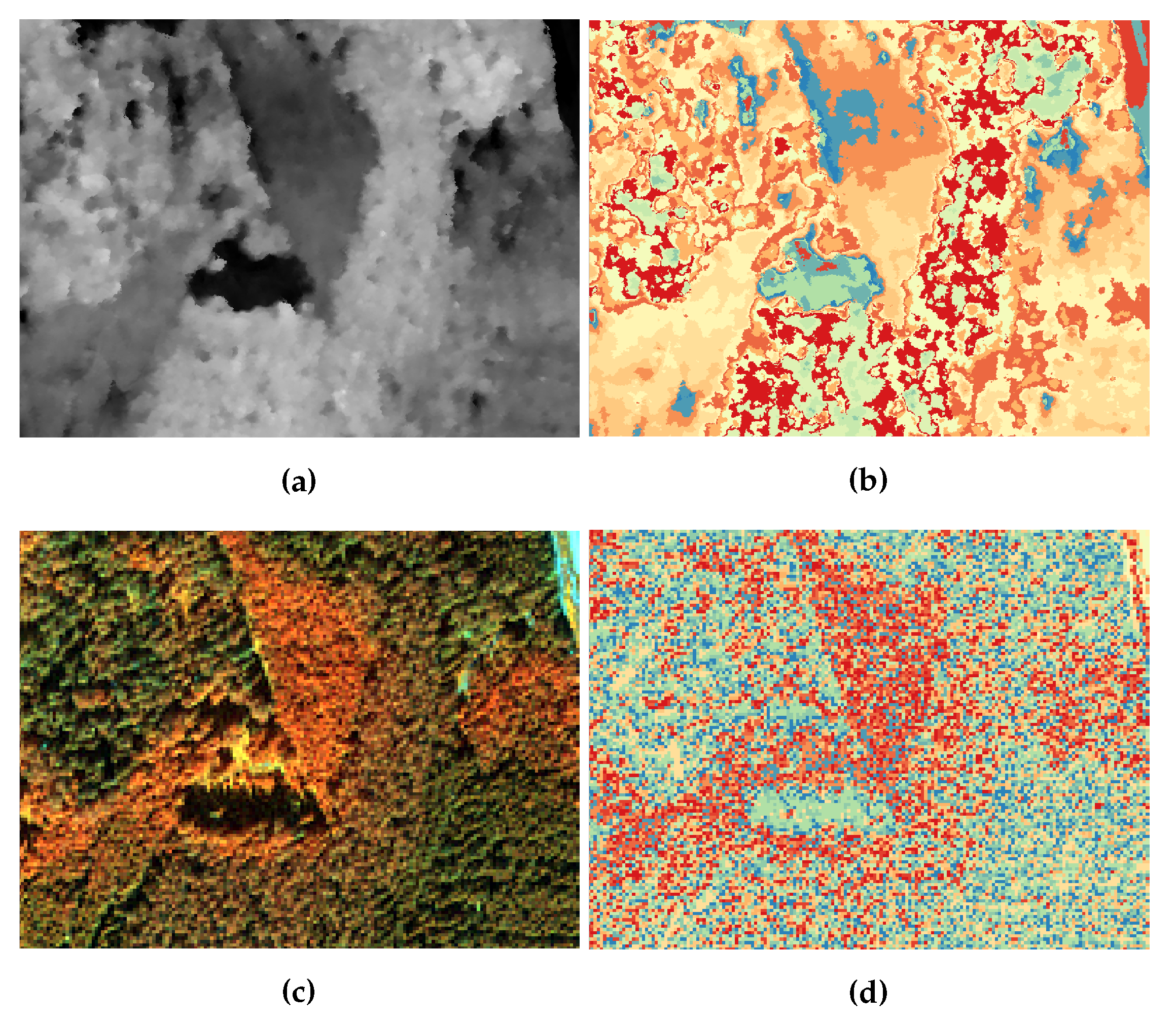
2.3.1. Modified JSEG Workflow

The JSEG describes local textures in the class-map image (see examples in Figure 2, created by k-means) using a variable J [30] calculated in a pixel neighbourhood specified by the window size. Higher J values indicate higher heterogeneity of the texture within a neighbourhood. Then, the region-growing algorithm was initialised by seed regions. Seed regions were found using a workflow based on thresholding, which selects areas with low J values, indicating potentially uniform textures. The region growing can be employed by combining J images of varying window sizes. For example, region seeds can be found using the J image of a larger window size, while the pixel-by-pixel region growing can be performed using some of the J images of smaller window sizes.

We modified the JSEG segmentation workflow described in [30], to incorporate sequential processing of the CHM and MS datasets.

The workflow for microstand delineation at a spatial resolution of 0.5 m/px includes the following steps:

• Calculate J images for clustered (number of clusters $k=16$) CHM at three scales with window sizes $w=33$ px, $w=17$ px, and $w=7$ px as $J{I}_{33}$, $J{I}_{17}$, and $J{I}_7$. The number of clusters was set by the trial-and-error method, aiming to emphasise microstands distinguishable by visual assessment. To emphasise sharp boundaries, the morphological gradient of the CHM with a $5\times 5$ square structuring element was merged with J images using the elementwise maximum operation;
• Perform the multiscale segmentation of J images. To save the calculation time, we excluded pixels with a CHM value lower than 3 m from further analysis, since we were interested only in the tree-covered areas;
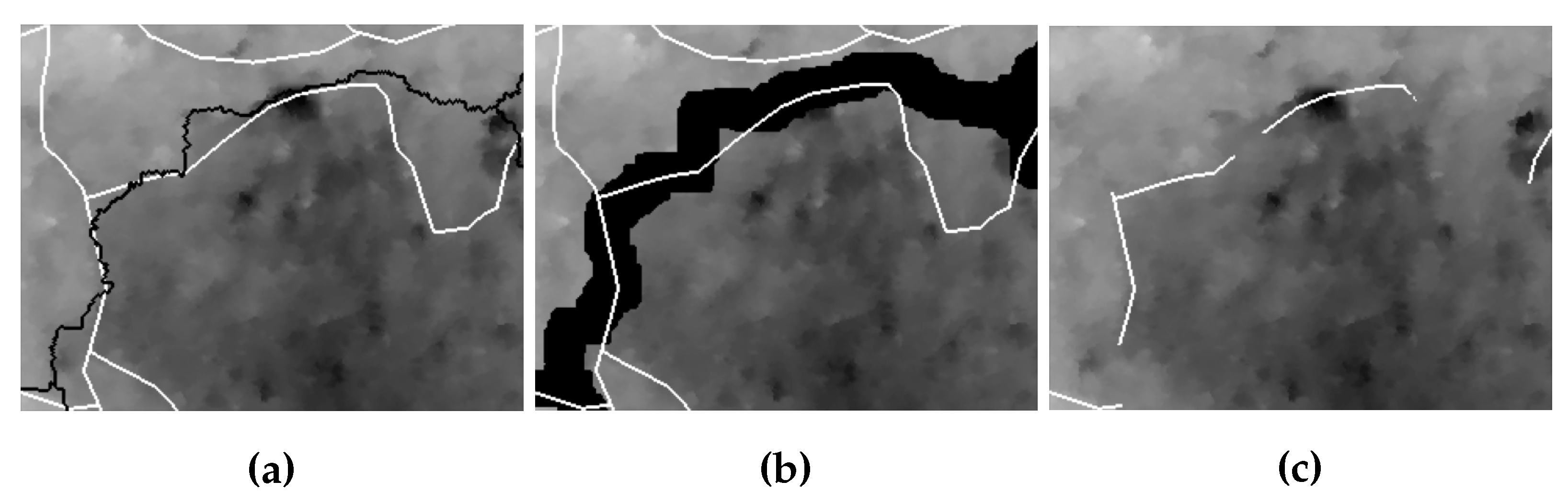
  • Scale 1: Find a seed image [30] using $J{I}_{33}$ by setting the minimum allowed seed size as 512 px. Add homogeneous chunks of $J{I}_{17}$ to the seed image, and perform region growing pixel-by-pixel using $J{I}_{17}$. The output is denoted as $R_{CHM1}$;
  • Scale 2: Find the refined seed image for $R_{CHM1}$ using $J{I}_{17}$ and 128 as the minimum allowed seed size; perform region growing by adding homogeneous chunks using $J{I}_7$; perform region growing pixel-by-pixel using $J{I}_7$. The output is denoted as $R_{CHM2}$;
• Calculate J images for the clustered ($k=16$) multispectral image (MS) at three scales with the same window sizes w = 33, 17, 7 as $J{I}_{MS33}$, $J{I}_{MS17}$, and $J{I}_{MS7}$;
• Resegment each region in $R_{CHM2}$. Statistical measures of the JSEG method were calculated for each region from $R_{CHM2}$ to be processed individually, and segmentation again was performed at multiple scales:

  (a)

  for the first scale $MS1$, find new seeds for the region using $J{I}_{MS33}$, and employ the pixel-by-pixel region growing using $J{I}_{MS17}$. The output is denoted as $R_{CHM2,MS1,JI33,JI17}$, where the first index shows the CHM segmentation scale, the second one reflects the MS scale, and the last ones indicate the J images employed;

  (b)

  For the second scale $MS2$, find new seeds for the segmented image from the previous Step (a) using $J{I}_{MS17}$ and perform the pixel-by-pixel region growing using $J{I}_{MS7}$. The output is denoted as $R_{CHM2,MS2,JI17,JI7}$;

  (c)

  If three scales are employed, find new seeds (64 as the minimum allowed seed size) for the output of Step (b) using $J{I}_{MS7}$, and apply the pixel-by-pixel region growing using $J{I}_{MS7}$. The output is denoted as $R_{CHM2,MS3,JI33,JI7,JI7}$;

• An optional step is merging regions smaller than the specified threshold with the most similar neighbour region, defining the similarity as the Euclidean distance between the trimmed mean values of the regions under consideration.

2.3.2. Generic Region Merging

The GRM algorithm of the Orfeo Toolbox (OTB) starts by considering each pixel as a separate segment and numbering it with a unique label. Adjacent segments are iteratively combined if they meet the homogeneity criterion. The OTB implementation offers several homogeneity criteria, but we employed the Baatz and Schape criterion [34]. The Baatz and Schape criterion measures spectral and spatial homogeneity before and after merging two adjacent segments. Adjacent segments are merged if the criterion value is below the threshold T specified by the user. Weight coefficients can be applied to put higher significance on spectral homogeneity $w_s$ or spatial compactness $w_c$.

We applied GRM to MS, the CHM images separately, and a fused dataset as well. Data fusion of 4 multispectral bands and the CHM was performed by simply adding the CHM as the fifth band in the image. The CHM was normalised by setting all height values larger than 50 m to 50 m and dividing the CHM by 50 to ensure values in the range $[0,1]$. Multispectral bands were normalised by dividing each band with its maximum value to keep values similarly distributed among the bands.

Figure 3 provides a small sample of the input data for GRM: GeoEye-1 false-colour image (NIR, green, blue as the red, green, blue layers), the GeoEye-1-based CHM and fused multiband image (NIR, green, the CHM were used for visualisation as the red, green, blue layers).

2.3.3. Microstand Quality Assessment

Unsupervised image segmentation is by nature an ill-defined problem with many potentially correct solutions [30]. Objects in the forests are not visually clearly separable, and the reference data also depend on the image analyst’s subjective opinions. Therefore, the reference dataset as well do not represent the sole and full-fledged solution [12]. Thus, finding the best segmentation algorithm or parameter combination according to numerical metrics is also challenging. Räsänen et al. [28] studied different direct supervised and system-level metrics for forest habitat mapping and concluded that different segmentation results were considered the best when different metrics were used.

We calculated 3 sets of metrics to capture different aspects of the segmentation results in hemiboreal forests: (1) unsupervised metrics characterizing internal homogeneity and intersegment heterogeneity, (2) direct, supervised overlap metrics with microstands delineated by the image analyst, and (3) the system-level RMSE for stand volume estimation using different segmentations as a basic spatial unit; see

Table 2. Accuracy metrics employed in this study. The last column shows if a higher or lower value indicates better segmentation: ↑—a higher metric value indicates higher quality, ↓—a lower metric value indicates higher quality.

Abbreviation	Metric	Group	Higher Accuracy
$wVarNor{m}_{CHM}$	Normalised height variance	Direct, unsupervised	↓
$S_{CHM}$	Average difference in mean height between adjacent microstands	Direct, unsupervised	↑
$S_{MS}$	Average Euclidean distance between the mean spectral vectors of adjacent microstands	Direct, unsupervised	↑
$S_{LMH}$	Average difference in mean heights of local maximums between adjacent microstands	Direct, unsupervised	↑
$OS$	Oversegmentation	Direct, supervised	↓
$US$	Undersegmentation	Direct, supervised	↓
D	Summary score	Direct, supervised	↓
$C_B$	Boundary similarity	Direct, supervised	↑
$RMSE$	Root-mean-squared error for stand volume estimation	System-level, supervised	↓

.

All metrics were calculated for the microstand segments and between forest microstand segments only if adjacent segments were analysed, not including segments belonging to other land cover types. Forest segments were selected by setting a height threshold to the CHM. A segment was considered a forest microstand only if its average GeoEye-1 CHM value was greater than or equal to 3 m. According to local legislation, a stand with an average height of at least 5 m is considered a forest. This threshold was reduced to consider the spacing between the trees and the lower parts of the tree crowns, which were included in the calculation of the average value.

Metric $wVarNor{m}_{CHM}$ characterises the height variance of the pixels belonging to the same microstand [21]. The upper bound of $wVarNor{m}_{CHM}$ is equal to 1 when the variance of the segment is equal to the variance of the whole segmented image, while the lower bound is 0 when all pixel values within a segment are the same. Lower values indicate higher internal homogeneity of the segments. This metric is unsuitable if gaps between trees are clearly visible in the CHM. Height values of those gaps would affect the height variance values, but those gaps are not undesirable in a microstand, if the stand density is low, but forms a regular macrotexture. We calculated $wVarNor{m}_{CHM}$ for GeoEye-1-based CHM, where individual tree crowns are not clearly visible.

Metric $S_f$ shows the average difference in feature f values between adjacent microstands (microstands with a common border):

$$S_f=\frac{{\sum }_{i=1}^n{\sum }_{j=1}^n{w}_{ij}\left(\right||f_i-f_j\left|\right|)}{\sum w_{ij}},$$

(1)

where n is the number of microstands;

$f_i$, $f_j$ is the average value of the feature f for microstand i and microstand j;

$w_{ij}=1$ if microstand numbers i and j have a common border and $i\ne j$, otherwise $w_{ij}=0$.

We employed several features: $S_{CHM}$, $S_{MS}$, and $S_{LMH}$. $S_{CHM}$ shows the average difference of the GeoEye-1-based mean CHM values of adjacent microstand pairs in metres, while $S_{MS}$ shows the average Euclidean distance between the mean spectral vectors of adjacent microstands. $S_{LMH}$ was calculated using the LiDAR-based CHM where individual tree crowns can be separated by simple local maximum filtering with a filter size of 3.5 m. $S_{LMH}$ shows the difference in the average local maximum height for adjacent microstands. Higher $S_f$ values indicate better segmentation results for all metrics because the neighbouring microstands are less similar in the context of forest-related features.

Supervised, direct polygon overlap metrics included $OS$, $US$, D, and $C_B$.

Oversegmentation ($OS$), undersegmentation ($US$), and summary score (D) explained in [21,35] were used as area-based metrics to characterise the overlap between microstand polygons delineated by the image analyst and the segmentation workflow. Thus, the values close to zero indicate higher accuracy, but those close to one indicate low accuracy.

We also calculated the boundary similarity metric $C_B$ similar to outline proportions within the buffer zones presented by Neubert and Herold [36]. Lucieer et al. [37] suggested calculating the average distance between a segment boundary pixel and the reference boundary ($D\left(b\right)$) to characterise the quality and dissimilarity of the borders. However, a visual comparison showed that there were cases where the border found by the workflow actually was more accurate than the border selected by the image analyst. In those cases, the average distance can give the impression of errors. A more accurate interpretation would be considering these offsets as natural differences between the border generalisation by a human interpreter and a pixel-by-pixel analysis of the computer method. Therefore, we used the metric $C_B$, which allows one to evaluate the percentage of the reference border located close to the segmentation borders (see Figure 4). It can be defined as follows:

$$C_B=\sum \left(B_{r}AND{B}_{m,dilated}\right)/\sum \left(B_r\right),$$

(2)

where $B_r$ is the rasterised reference boundary, one pixel thick at the same spatial resolution as the remote sensing dataset;

$B_m$ is the one-pixel-thick boundary created by the segmentation workflow. A binary dilation with a square structuring element of size $T\times T$ was employed to create a buffer zone around the boundary denoted by $B_{m,dilated}$.

The threshold T sets the spatial distance in which we still consider $B_r$ and segmentation border $B_m$ as well matched. In our study, we set $T=10$ m according to the visual assessment.

Finally, the system-level assessment was performed by applying the random forest regressor [38] for stand volume estimation at the microstand level using the NFI data as the ground truth. If the microstand overlaps with the forest compartment by more than 50%, then the stand volume of the dominant tree species within the forest compartment is assigned to the microstand; otherwise, the microstand is not used for further processing. Each of the microstands was described by the following remote sensing data features: mean values of 4 GeoEye-1 spectral bands, the GeoEye-1 CHM mean value and standard deviation, the number of local maximums in the LGIA CHM (maximum filter size 7 m), and the average height value of local maximums in the LGIA CHM. As a result, each microstand was characterised by 8 features.

The described microstands with assigned reference stand volume values were split into training and test datasets using 70% for fitting the random forest and 30% for testing. Once random forest predictions for the test set were made, the RMSE was calculated as a quality metric. A lower RMSE indicates lower prediction errors. As microstands were employed as the basic spatial units, a lower RMSE for the segmentation case would indicate a better segmentation result for stand volume estimation purposes.

2.3.4. Adjusting Workflow Parameters

Parameters for the JSEG-based workflow were set based on a visual assessment to produce segments as similar as possible to the segments delineated by the image analyst.

Parameters for the GRM-based workflow were adjusted using computational parameter tests. In the parameter tests, all meaningful combinations of the most important GRM parameters T, $w_s$, and $w_c$ were tested. The two best segmentation results for each dataset were produced using two different optimisation criteria:

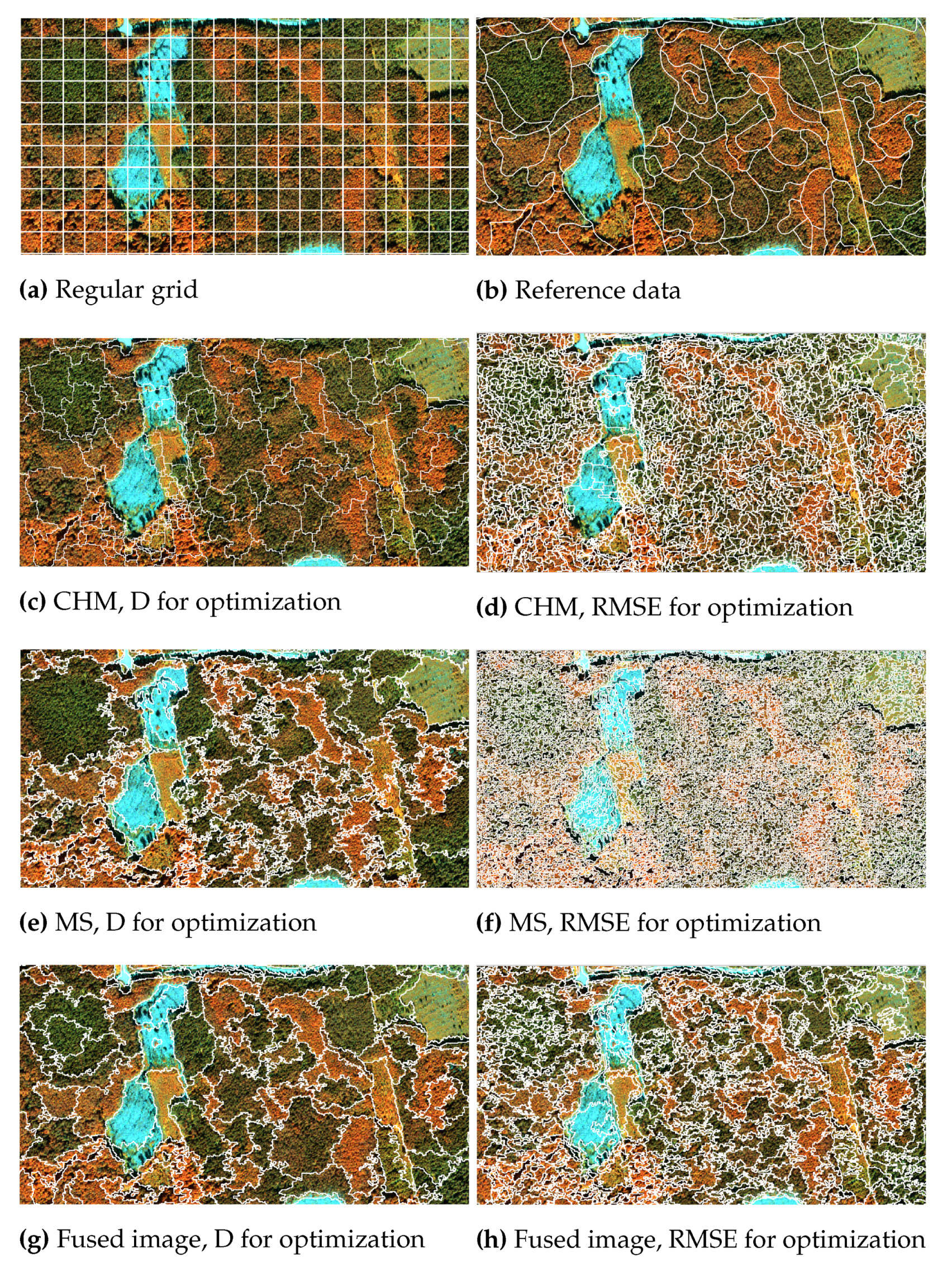
• D: lowest D score showing the best match with segments delineated by the image analyst;
• $RMSE$: lowest $RMSE$ when segments are employed as the basic spatial units for stand volume estimation.

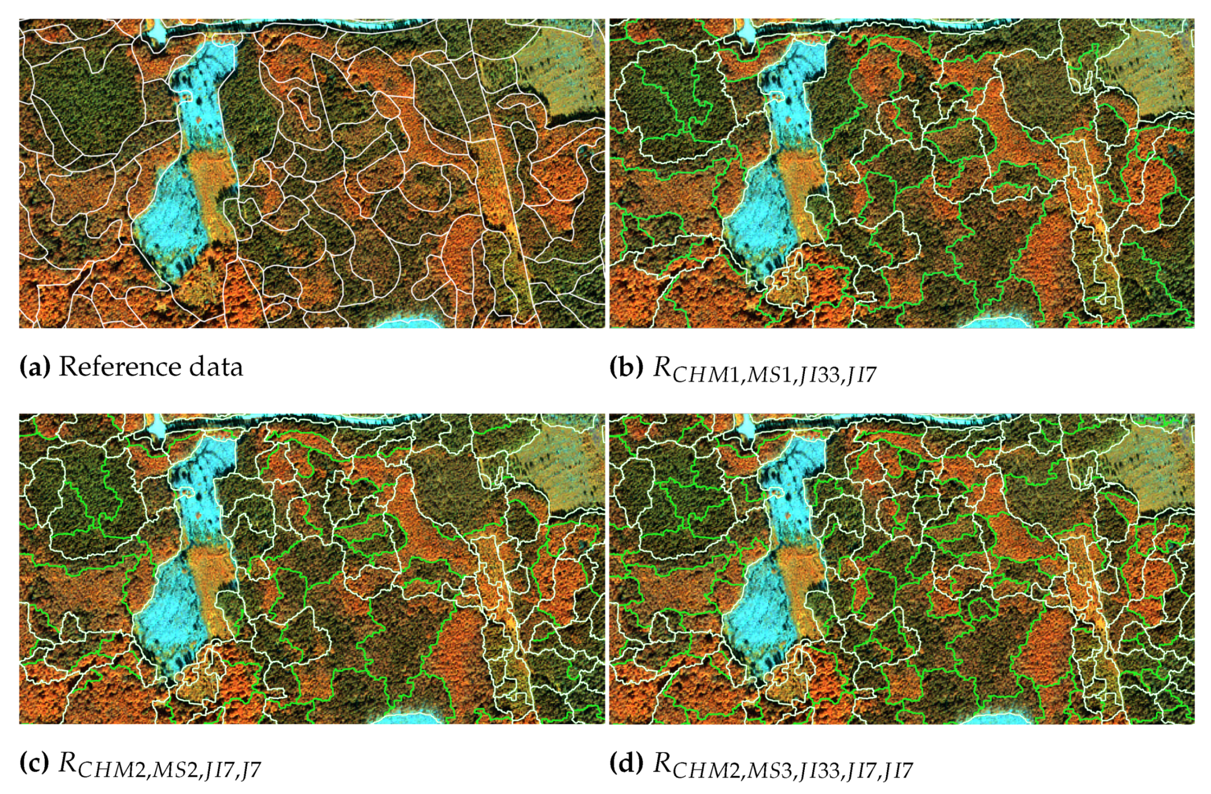
Due to a large amount of VHR data in our study site, we applied data parallelism to the segmentation workflows by splitting the dataset into 1 km × 1 km tiles according to the local map page division nomenclature and by processing each tile in a separate process. Of course, data splitting results in visible tile boundaries, also in the segmentation results, which could be avoided by adding postprocessing to the workflows. However, in our study, tile borders were not additionally processed.

3. Results

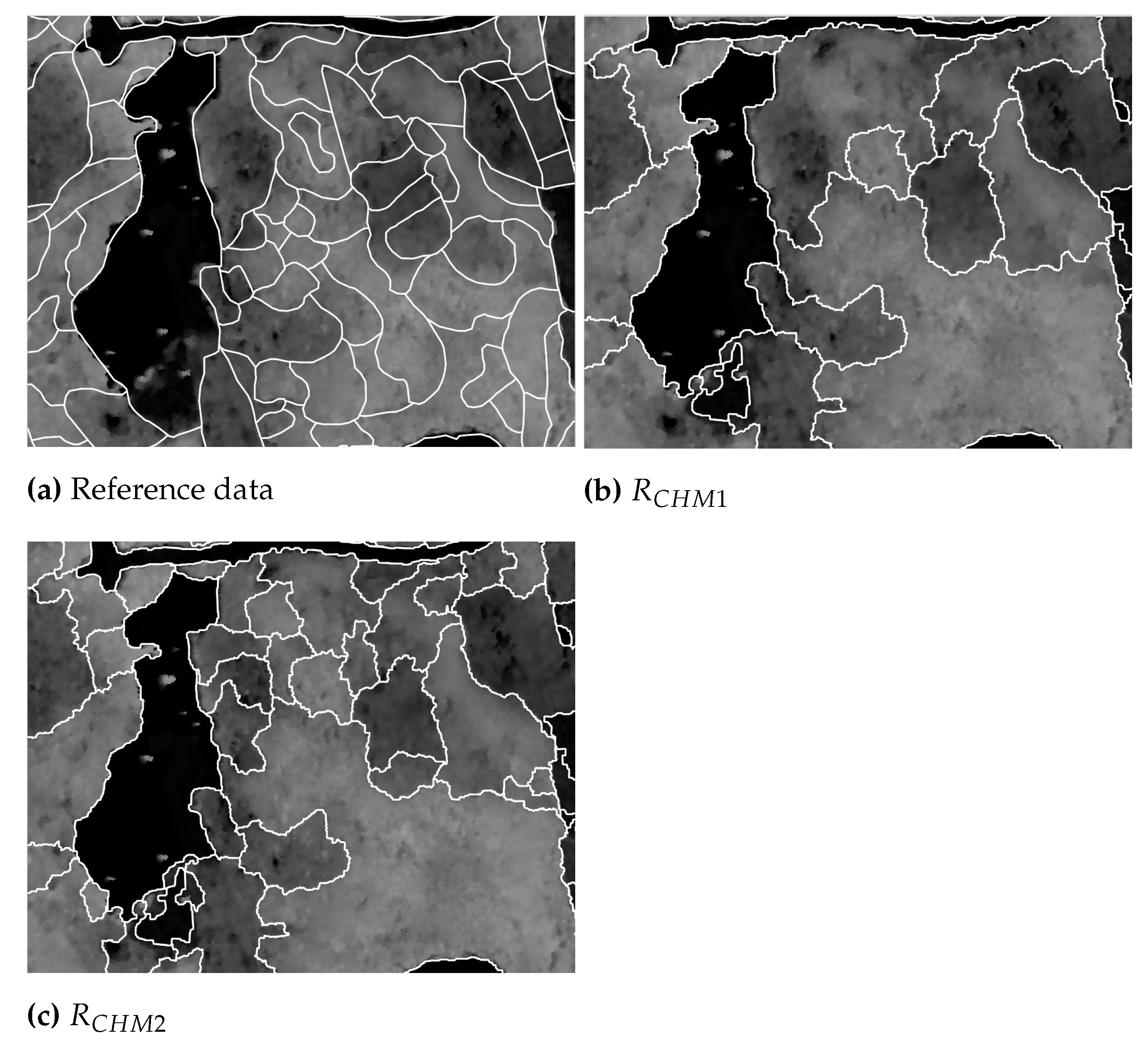
3.1. Examples of the Segmentation Results

Figure 5 shows an example of the first stage of JSEG segmentation using only the CHM as the input. It can be seen that the JSEG segmentation can efficiently capture smooth borders between microstands of different heights, and $R_{CHM2}$ seems to be a visually better match to the reference data.

Figure 6 shows examples of the JSEG results when the multispectral data segmentation was added to the CHM segmentation. Green borders in the image confirm how the complementary nature of height information in the CHM and spectral information in the satellite images allowed one to include significant aspects of microstands. Similar height classes were extracted from the CHM, but the coniferous and deciduous tree species and the tree crown closure as a macrotexture were extracted from the multispectral images.

Figure 7 shows an example of the GRM tests with different dataset combinations (CHM, MS, and fused images) and optimisation criteria (D and RMSE; see Section 2.3.4) for the adjustment of the algorithm parameters, as well as a sample of the image analyst’s segmentation and the regular grid. When optimisation concerning D was applied, we could observe meaningful segments, however different from the delineation results of the human analyst. Meanwhile, optimisation concerning the RMSE resulted in a strong oversegmentation.

Visual comparison of GRM and JSEG showed that the usage of J images for segmentation resulted in smoother region boundaries; in contrast, the GRM results required boundary regularisation in postprocessing or should be applied using even lower-spatial-resolution images.

3.2. Unsupervised Metrics

Table 3. Unsupervised metrics. Arrows ↓ and ↑ indicate whether a lower or higher value is considered as better. The best value for each metric is emphasised with bold font.

Case	${\mathit{vWarNorm}}_{\mathit{CHM}}\downarrow$	${\mathit{S}}_{\mathit{CHM}}\uparrow$	${\mathit{S}}_{\mathit{MS}}\uparrow$	${\mathit{S}}_{\mathit{LMH}}\uparrow$
Regular grid $48\times 48$ m	0.35	3.9	9.32	2.83
Reference polygons	0.24	5.68	934	4.2
GRM CHM, D	0.09	7.47	569	4.34
GRM CHM, RMSE	0.01	4.86	31	3.09
JSEG CHM	0.12	8.2	103	4.4
GRM MS, D	0.35	4.3	638	3.8
GRM MS, RMSE	0.3	2.63	23.7	2.4
JSEG MS	0.25	4.2	223	4.1
GRM fused, D	0.14	6.53	822	4.27
GRM fused, RMSE	0.1	4.92	173	3.18
JSEG fused	0.09	7.1	106	4.9

summarises the unsupervised metric values for the JSEG and GRM workflows, as well as for regular grid cells and the segmentation by the image analyst. The abbreviations CHM, MS, and fused (both the CHM and MS) explain the dataset used for segmentation, but the D and RMSE reflect the optimisation criteria used to the adjust workflows’ parameters.

The internal heterogeneity of the segments $vWarNor{m}_{CHM}$ with respect to the CHM was naturally higher for the regular grid and for those experiments performed using multispectral information only. When the CHM was included in the segmentation process, both segmentation algorithms achieved higher internal segment homogeneity than the image analyst.

Differences between stand-specific segment characteristics $S_f$ were higher for tests optimised by the D criterion, but significantly lower for tests where the optimisation using the RMSE of stand volume estimation was performed. The GRM and JSEG algorithms for the fused dataset showed the best performance. GRM in all cases captured multispectral differences between stands better, while JSEG segmentation resulted in higher height differences between adjacent microstands.

3.3. Supervised and System-Level Metrics

The supervised direct and system-level metrics are summarised in

Table 4. Supervised metrics. Arrows ↓ and ↑ indicate whether a lower or higher value is considered better. The best value for each metric is emphasised with bold font.

Case	$\mathit{OS}\downarrow$	$\mathit{US}\downarrow$	$\mathit{D}\downarrow$	${\mathit{C}}_{\mathit{B}}\uparrow$	$\mathit{RMSE}\downarrow$	$\mathit{avgA}$	$\mathit{stdA}$
Regular grid $48\times 48$ m	0.63	0.45	0.55	0.5	74.8	1369	0
Reference polygons	-	-	-	-	67.9	1352	362
GRM CHM, D	0.38	0.5	0.45	0.67	82	890	425
GRM CHM, RMSE	0.89	0.15	0.63	0.99	78.8	66	12
JSEG CHM	0.63	0.43	0.54	0.69	80.1	586	572
GRM MS, D	0.51	0.54	0.53	0.76	80.6	833	326
GRM MS, RMSE	0.94	0.11	0.67	0.99	78.9	38	8
JSEG MS	0.61	0.45	0.75	0.75	82	620	535
GRM fused, D	0.38	0.52	0.46	0.74	82	1104	416
GRM fused, RMSE	0.71	0.3	0.55	0.94	78.8	271	55
JSEG fused	0.71	0.43	0.54	0.79	76.0	651	114

. In addition, the average segment area $avgA$ and standard deviation of the segment area $stdA$ are shown as well.

The lowest RMSE = 67.9 m${}^3$/ha was achieved by using the image analyst’s selection. However, in this case, the regression task was performed only for six sample areas containing a smaller number of segments. Other tests were performed in the whole study site with a large number of segments. For example, the GRM fused test included 10,422 segments for training random forest regression and 4467 segments for testing. In comparison, only 1890 segments were available for training and 810 for testing in the case of the image analyst’s selection.

Table 4 shows that the stand volume estimation error was minimally affected by the segmentation results. The RMSE varied within a range of 6 m${}^3$/ha showing RMSE = 76.0 m${}^3$/ha for JSEG applied to the fused dataset and RMSE = 78.8 m${}^3$/ha for GRM applied to the fused dataset as well. However, this small difference does not show a practical gain of data fusion already in the segmentation stage, since an even smaller error RMSE = 74.8 m${}^3$/ha was achieved by performing no segmentation at all and using regular grid patches as a basic spatial unit for stand volume estimation.

Comparing the overlap metrics between the results of the segmentation algorithms and the image analyst, one can observe that the summary score D was quite high for all outputs, indicating that the areas of the microstands found by the workflows were noticeably different from those found by the image analyst, however similar in size. Optimisation tests with respect to the RMSE showed clear trends of oversegmentation. The mutually similar OS and US scores for outputs with the multispectral information added characterised only different segmentation results without clear trends in oversegmentation or undersegmentation.

Meanwhile, the coincidence of the boundaries $C_B$ was high, indicating that significant transitions were found even in the presence of different polygon shapes. However, the $C_B$ metric was also affected by oversegmentation, which led to a higher border matching score. Considering only the JSEG results and GRM results with D as the optimisation criteria, 76–79% of the borders found by the image analyst were also found using automatic segmentation methods.

We found no correlations between the border matching score and forest inventory parameters such as tree species, stand volume, and stand density. Still,

Table 5. $C_B$ values for the CHM segmentation using the JSEG workflow at two scales.

Site No.	Average ${\mathit{C}}_{\mathit{B}}$ for ${\mathit{R}}_{\mathbf{CHM}1}$	Std of ${\mathit{C}}_{\mathit{B}}$ for ${\mathit{R}}_{\mathbf{CHM}1}$	Average ${\mathit{C}}_{\mathit{B}}$ for ${\mathit{R}}_{\mathbf{CHM}2}$	Std of ${\mathit{C}}_{\mathit{B}}$ for ${\mathit{R}}_{\mathbf{CHM}2}$	Confidence Level of the Image Analyst
1	0.49	0.04	0.56	0.03	0.73
2	0.41	0.08	0.51	0.06	0.70
3	0.35	0.05	0.44	0.01	0.67
4	0.34	0.1	0.43	0.08	0.67
5	0.41	0.05	0.49	0.03	0.7
6	0.45	0.07	0.52	0.07	0.72

shows a mild correlation between $C_B$ and the level of confidence of the image analyst in different sample areas. Metric $C_B$ was slightly lower for sample areas where the image analyst reported lower confidence levels indicating complex forest structures. A visual assessment of those study sites showed that Areas 1 and 6 were subject to intensive management with frequent, clearly visible rectangular compartments divided by rides, roads, and ditches, but Areas 3 and 4 were very inhomogeneous. The higher confidence level for Area 3 might be explained by subjectivity factors. It was the first study site to be processed by the image analyst, and further work process and communication with remote sensing specialists might have changed this evaluation.

4. Discussion

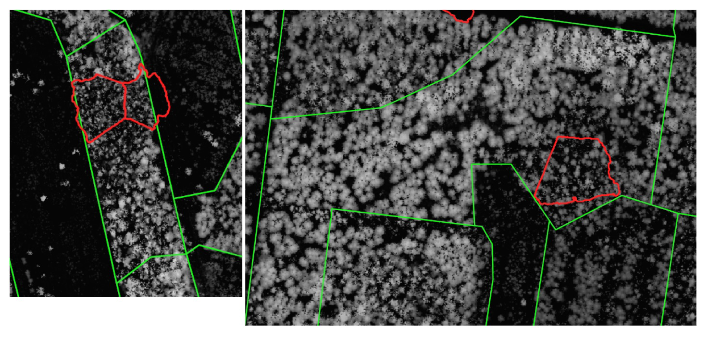
4.1. Applicability for Microstand Border Refinement

A visual assessment of the workflow segments confirmed that meaningful and relevant microstands were separated by both workflows. However, the segments were visually different from those selected by the image analyst. This was already expected because microstand segmentation is ill-defined with many correct solutions.

Considering oversegmentation $OS$, undersegmentation $US$, and the summary score D, those values for our study were higher than presented by Sanchez-Lopez et al. [21], but these differences could also be caused by differences in the spatial resolution of the datasets used in our study and the study of [21].

Since microstands in many cases cannot be unambiguously defined even by a human interpreter and fieldwork, the $C_B$ measure is an efficient metric to measure the ability of the workflow to find significant borders even in the presence of oversegmentation. However, since a buffer zone is created around the algorithm border, $C_B$ can show higher values only due to oversegmentation. Therefore, the width of the buffer zone has to be taken into consideration when analysing the values of $C_B$. A larger buffer zone can cause a risk of unreasonably increasing $C_B$, while a too-small buffer zone does not include the possible delineation inaccuracies of the image analyst.

In general, the unsupervised metrics showed better values for the JSEG and GRM workflows than for the selection of the image analyst. This could be explained by border generalisation when microstands are selected by hand, while the data processing workflows without additional modules for generalisation draw borders at the pixel scale. Finer borders might result in higher internal segment homogeneity and higher average differences between adjacent segments. The study by [17] evaluated an internal homogeneity metric, normalised variance (the normalisation methodology was different than in our study), on a 1 m${}^2$ grid and obtained higher values. However, this could be explained by both the different normalisation methodology and higher heterogeneity of LiDAR-based metrics.

Many authors acknowledge that segmentation accuracy metrics describe only certain aspects of segments [28,35,39], but there are no metrics that can unambiguously determine the best segmentation result. Varo-Martínez et al. [17] specified that metric sets should be established for certain tasks, for example precision silviculture requires very precise stand delineation regarding intra-region variance.

4.2. Applicability to the Stand Volume Estimation Task

Our study showed that segments produced by different algorithms, datasets, and algorithm parameters have a small impact on the stand volume estimation accuracy, suggesting that other factors are setting limits to reduced the RMSE instead of segment delineation. The same conclusion about different datasets, including LiDAR and hyperspectral data, were also made by Dechesne et al. [26]. Moreover, even using regular grid patches as a basic spatial unit resulted in a lower error of the random forest regressor.

The RMSE values in our tests were similar (74.8 m${}^3$/ha ⩽ RMSE ⩽ 80.6 m${}^3$/ha, $nRMSE\approx 13\%$ using 600 m${}^3$/ha as the maximal stand volume) to those acquired in other studies reviewed by Surovỳ and Kuželka [40].

The lack of significant fluctuations in the RMSE between different tests and better results using regular grid patches raise a question about potential error sources. The classification accuracy also had a small variation in the study of Räsänen et al. [28], providing evidence of the robustness of object-based methodology, meaning that good classification accuracy can be obtained even if the segmentation is not the best possible.

However, in our study, the RMSE limits might be determined by the reference data compatibility with microstands or grid patches as the spatial units (see Figure 8) and erroneous entries in the NFI database. The stand volume value for a forest compartment is obtained by the summation of the values for microstands within this compartment. Since the forest compartment boundaries are also affected by management factors and historical reasons, compartments are more heterogeneous than microstands. Therefore, in the case of mixed compartments, even stand volume values for dominant tree species are not valid reference data for much more homogeneous microstands, introducing errors both in training and testing. The solution could be to increase the study area to a much larger region and use only pure NFI compartments (with one dominant tree species of a similar age) to capture the correct ground truth accounting for natural variations in tree species and age. Since the RMSE was used just as one metric to evaluate the segmentation quality, the workflow for stand volume estimation was also simplified, and more studies about the error sources in the stand volume estimation would be required.

The higher accuracy obtained using regular grid patches could be caused by the reduced variance of the feature values when the spatial unit is without any size variations. The optimisation procedure for GRM tended to achieve lower RMSEs when oversegmentation was applied with a higher emphasis on spectral homogeneity. Thus, the unsupervised metrics already allowed us to conclude that oversegmentation is not an undesirable phenomenon, if the segments are further planned to be used as basic units for forest inventory parameter estimation tasks. Still, differences between tests showed variation in a range of no more than 7 m${}^3$.

5. Conclusions

Microstands can serve as robust spatial processing units for an automated remote-sensing-based forest inventory and for increasing the accuracy of microstand borders used in the traditional forest inventory. GeoEye-1 stereo data give a great opportunity to acquire both spectral and height information, which is up-to-date and coincident in time.

Metrics characterizing overlap between the workflow segments and segments produced by the image analyst showed that 76–79% of significant borders were also found by the segmentation methods; however, the segment geometry itself was different.

In future studies, we would recommend changing the accuracy assessment procedure by offering workflow-produced segments for review to several independent image analysts instead of requiring the image analysts to delineate microstands themselves. Then, those workflow segments could be analysed visually and assessed as useful ones in daily forest inventory or invalid segments specifying why a segment cannot be used for practical microstand border refinement. Since we found no correlations between forest inventory parameters and the confidence level assigned by the image analyst, the reason for the low confidence would give valuable information about the further development of the workflows. This might also give more appropriate insight into the practical applicability of segmentation for border refinement because the visual interpretation of the segmentation results confirmed meaningful microstand propositions.

Stand volume estimation tests showed no benefits of using segments instead of just regular grid patches as a basic spatial unit. The best RMSE = 74.8 m ${}^3$/ha was achieved by using regular grid patches. This could be explained by the actual incompatibility between the stand volume format in the NFI and required for using microstands as a basic spatial unit.

The GRM workflow efficiently captures borders in multispectral data, but the JSEG workflow is more efficient on tree crown macrotexture delineation.

Both segmentation approaches would be useful for preparing ready-to-use microstand maps, but the accuracy assessment procedure should be switched to one including direct visual analysis of workflow segments. For stand volume estimations using the microstand as a basic spatial unit, tests should be repeated using a much larger study site and only forest compartments with a homogeneous structure.

References

1. Dechesne, C.; Mallet, C.; Le Bris, A.; Gouet-Brunet, V. Remote sensing technologies for enhancing forest inventories: A review. Can. J. Remote Sens. 2016, 42, 619–641. [Google Scholar]
2. Latvian Geospatial Information Agency, Ortofotokartes. Available online: https://www.lgia.gov.lv/lv/ortofotokartes-0 (accessed on 5 January 2022). (In Latvian)
3. Barrett, F.; McRoberts, R.E.; Tomppo, E.; Cienciala, E.; Waser, L.T. A questionnaire-based review of the operational use of remotely sensed data by national forest inventories. Remote Sens. Environ. 2016, 174, 279–289. [Google Scholar] [CrossRef]
4. Schumacher, J.; Rattay, M.; Kirchhöfer, M.; Adler, P.; Kändler, G. Combination of multi-temporal sentinel 2 images and aerial image based canopy height models for timber volume modelling. Forests 2019, 10, 746. [Google Scholar] [CrossRef] [Green Version]
5. Kankare, V.; Holopainen, M.; Vastaranta, M.; Liang, X.; Yu, X.; Kaartinen, H.; Hyyppä, J. Outlook for the Single-Tree-Level Forest Inventory in Nordic Countries; Springer: New York, NY, USA, 2017. [Google Scholar]
6. Pascual, A.; Pukkala, T.; de Miguel, S.; Pesonen, A.; Packalen, P. Influence of size and shape of forest inventory units on the layout of harvest blocks in numerical forest planning. Eur. J. For. Res. 2019, 138, 111–123. [Google Scholar] [CrossRef] [Green Version]
7. Bergseng, E.; Ørka, H.O.; Næsset, E.; Gobakken, T. Assessing forest inventory information obtained from different inventory approaches and remote sensing data sources. Ann. For. Sci. 2015, 72, 33–45. [Google Scholar] [CrossRef] [Green Version]
8. Ke, Y.; Quackenbush, L.J. A review of methods for automatic individual tree-crown detection and delineation from passive remote sensing. Int. J. Remote Sens. 2011, 32, 4725–4747. [Google Scholar] [CrossRef]
9. Tianyang, D.; Jian, Z.; Sibin, G.; Ying, S.; Jing, F. Single-tree detection in high-resolution remote-sensing images based on a cascade neural network. ISPRS Int. J. Geo-Inf. 2018, 7, 367. [Google Scholar] [CrossRef] [Green Version]
10. Tianyang, D.; Jian, Z.; Sibin, G.; Ying, S.; Jing, F. Local pivotal method sampling design combined with micro stands utilizing airborne laser scanning data in a long term forest management planning setting. Silva Fenn 2015, 50, 1414. [Google Scholar]
11. Legal Acts of the Republic of Latvia, Law on Forests. Available online: https://likumi.lv/ta/en/en/id/2825 (accessed on 5 January 2022).
12. Koch, B.; Straub, C.; Dees, M.; Wang, Y.; Weinacker, H. Airborne laser data for stand delineation and information extraction. Int. J. Remote Sens. 2009, 30, 935–963. [Google Scholar] [CrossRef]
13. von Gadow, K.; Pukkala, T. Designing Green Landscapes; Springer Science & Business Media: New York, NY, USA, 2008; Volume 15. [Google Scholar]
14. Baatz, M.; Schape, A. Multi Resolution Segmentation: An Optimum Approach for High Quality Multi Scale Image Segmentation; Wichmann-Verlag: Heidelberg, Germany, 2000; pp. 12–23. [Google Scholar]
15. Ozkan, U.Y.; Demirel, T.; Ozdemir, I.; Saglam, S.; Mert, A. Examining lidar-worldview-3 data synergy to generate a detailed stand map in a mixed forest in the north-west of Turkey. Adv. Space Res. 2020, 65, 2608–2621. [Google Scholar] [CrossRef]
16. Rajbhandari, S.; Aryal, J.; Osborn, J.; Lucieer, A.; Musk, R. Leveraging machine learning to extend Ontology-driven Geographic Object-Based Image Analysis (O-GEOBIA): A case study in forest-type mapping. Remote Sens. 2019, 11, 503. [Google Scholar] [CrossRef] [Green Version]
17. Varo-Martínez, M.Á.; Navarro-Cerrillo, R.M.; Hernández-Clemente, R.; Duque-Lazo, J. Semi-automated stand delineation in mediterranean pinus sylvestris plantations through segmentation of lidar data: The influence of pulse density. Int. J. Appl. Earth Obs. Geoinf. 2017, 56, 54–64. [Google Scholar] [CrossRef] [Green Version]
18. Leppänen, V.J.; Tokola, T.; Maltamo, M.; Mehtätalo, L.; Pusa, T.; Mustonen, J. Automatic delineation of forest stands from lidar data. GEOBIA 2008, 1, 5–8. [Google Scholar]
19. Radoux, J.; Defourny, P. A quantitative assessment of boundaries in automated forest stand delineation using very high resolution imagery. Remote Sens. Environ. 2007, 110, 468–475. [Google Scholar] [CrossRef]
20. Hernando, A.; Tiede, D.; Albrecht, F.; Lang, S. Spatial and thematic assessment of object-based forest stand delineation using an ofa-matrix. Int. J. Appl. Earth Obs. Geoinf. 2012, 19, 214–225. [Google Scholar] [CrossRef] [Green Version]
21. Sanchez-Lopez, N.; Boschetti, L.; Hudak, A.T. Semi-automated delineation of stands in an even-age dominated forest: A lidar-geobia two-stage evaluation strategy. Remote Sens. 2018, 10, 1622. [Google Scholar] [CrossRef] [Green Version]
22. Zhao, P.; Gao, L.; Gao, T. Extracting forest parameters based on stand automatic segmentation algorithm. Sci. Rep. 2020, 10, 1571. [Google Scholar] [CrossRef] [Green Version]
23. Wu, Z.; Heikkinen, V.; Hauta-Kasari, M.; Parkkinen, J.; Tokola, T. Als data based forest stand delineation with a coarse-to-fine segmentation approach. In Proceedings of the 2014 7th International Congress on Image and Signal Processing, Dalian, China, 14–16 October 2014; pp. 547–552. [Google Scholar]
24. Bruggisser, M.; Hollaus, M.; Wang, D.; Pfeifer, N. Adaptive framework for the delineation of homogeneous forest areas based on lidar points. Remote Sens. 2019, 11, 189. [Google Scholar] [CrossRef] [Green Version]
25. Leckie, D. Stand delineation and composition estimation using semi-automated individual tree crown analysis. Remote Sens. Environ. 2003, 85, 355–369. [Google Scholar] [CrossRef]
26. Dechesne, C.; Mallet, C.; Le Bris, A.; Gouet-Brunet, V. Forest stand extraction: Which optimal remote sensing data source(s)? In Proceedings of the IGARSS 2018—2018 IEEE International Geoscience and Remote Sensing Symposium, Valencia, Spain, 22–27 July 2018; pp. 7279–7282. [Google Scholar]
27. Jia, W.; Sun, Y.; Pukkala, T.; Jin, X. Improved cellular automaton for stand delineation. Forests 2020, 11, 37. [Google Scholar] [CrossRef] [Green Version]
28. Räsänen, A.; Rusanen, A.; Kuitunen, M.; Lensu, A. What makes segmentation good? A case study in boreal forest habitat mapping. Int. J. Remote Sens. 2013, 34, 8603–8627. [Google Scholar] [CrossRef]
29. Wulder, M.A.; White, J.C.; Hay, G.J.; Castilla, G. Towards automated segmentation of forest inventory polygons on high spatial resolution satellite imagery. For. Chron. 2008, 84, 221–230. [Google Scholar] [CrossRef]
30. Deng, Y.; Manjunath, B. Unsupervised segmentation of color-texture regions in images and video. IEEE Trans. Pattern Anal. Mach. Intell. 2001, 23, 800–810. [Google Scholar] [CrossRef] [Green Version]
31. Petrokas, R.; Baliuckas, V.; Manton, M. Successional categorization of european hemi-boreal forest tree species. Plants 2020, 9, 1381. [Google Scholar] [CrossRef] [PubMed]
32. Wang, C.; Shi, A.-Y.; Wang, X.; Wu, F.M.; Huang, F.C.; Xu, L.Z. A novel multi-scale segmentation algorithm for high resolution remote sensing images based on wavelet transform and improved jseg algorithm. Optik 2014, 125, 5588–5595. [Google Scholar] [CrossRef]
33. European Space Imaging, “Geoeye-1”. Available online: https://www.euspaceimaging.com/geoeye-1/ (accessed on 5 January 2022).
34. Happ, P.; Ferreira, R.S.; Bentes, C.; Costa, G.A.O.P.; Feitosa, R.Q. Multiresolution segmentation: A parallel approach for high resolution image segmentation in multicore architectures. Int. Arch. Photogramm. Remote Sens. Spatial Inf. Sci. 2010, 38, C7. [Google Scholar]
35. Clinton, N.; Holt, A.; Scarborough, J.; Yan, L.I.; Gong, P. Accuracy assessment measures for object-based image segmentation goodness. Photogramm. Eng. Remote Sens. 2010, 76, 289–299. [Google Scholar] [CrossRef]
36. Neubert, M.; Herold, H. Assessment of remote sensing image segmentation quality. Development 2008, 10, 2007. [Google Scholar]
37. Lucieer, A.; Stein, A. Existential uncertainty of spatial objects segmented from satellite sensor imagery. IEEE Trans. Geosci. Remote Sens. 2002, 40, 2518–2521. [Google Scholar] [CrossRef] [Green Version]
38. Scikit-Learn Developers, “Scikit-Learn User Guide: Random Forest Regressor”. Available online: https://scikit-learn.org/stable/modules/generated/sklearn.ensemble.RandomForestRegressor.html (accessed on 5 January 2022).
39. Hay, G.J.; Castilla, G. Geographic object-based image analysis (geobia): A new name for a new discipline. In Object-Based Image Analysis; Springer: New York, NY, USA, 2008; pp. 75–89. [Google Scholar]
40. Surovỳ, P.; Kuželka, K. Acquisition of forest attributes for decision support at the forest enterprise level using remote-sensing techniques—A review. Forests 2019, 10, 273. [Google Scholar] [CrossRef] [Green Version]
Figure 1. Study site and six sample plots that were employed for additional reference data acquisition. Centre coordinates 56.46 ° N, 25.04 ° E.
Remotesensing 14 01471 g001
Figure 2. Examples of class-map images. (a) GeoEye-1-based CHM, (b) class-map image of (a) if 16 clusters are sought by k-means, (c) GeoEye-1-based false colour image (NIR, green, blue), and (d) class-map image of (c) if 16 clusters are sought by k-means.
Remotesensing 14 01471 g002
Figure 3. Example of GeoEye-1 dataset combinations: (a) false-colour MS image (NIR, green, blue as the image layers), (b) the CHM derived from the GeoEye-1 scene, and (c) fused multiband input for GRM (NIR, green, CHM as the image layers).
Remotesensing 14 01471 g003
Figure 4. Example showing the interpretation of C B . The length of B r in the extent is 1775 px; the length of B m = 1185 px; the matched border length is 658 px, C B = 37 % . (a) The CHM as the background layer; reference border B r marked with white line, segmentation border B m with black. (b) Segmentation border B m , d i l a t e d (in black) dilated with a square structuring element. (c) B r A N D B m , d i l a t e d : fragments of the microstand border selected by the image analyst that are located close to the microstand border marked by the data processing workflow.
Remotesensing 14 01471 g004
Figure 5. Example of the CHM segmentation using the JSEG workflow without adding the multispectral information (56.51 ° N, 24.96 ° E: 56.51 ° N, 24.97 ° E). (a) Reference data delineated by the image analyst, (b) R C H M 1 (see Section 2.3.1) segmentation results, and (c) R C H M 2 (see Section 2.3.1) segmentation results.
Remotesensing 14 01471 g005
Figure 6. Example of segmentation results using the JSEG workflow with multispectral information added (56.51 ° N, 24.96 ° E: 56.51 ° N, 24.97 ° E; the notation is described in Section 2.3.1). The white line denotes the CHM segmentation results, and the green one denotes the lines added during multispectral data processing. Background layer: GeoEye-1 satellite image (NIR, G, and B bands).
Remotesensing 14 01471 g006
Figure 7. Examples of different segmentation results using GRM (56.51 ° N, 24.96 ° E: 56.51 ° N, 24.97 ° E): (a) regular grid 48 × 48 m, (b) microstands delineated by the image analyst, (c) GRM results using only the GeoEye-1 CHM and D as the optimisation criteria, (d) GRM results using only the GeoEye-1 CHM and the R M S E as the optimisation criteria, (e) GRM results using only the 4 GeoEye-1 bands and D as the optimisation criteria, (f) GRM results using only the 4 GeoEye-1 bands and the R M S E as the optimisation criteria, (g) GRM results using combined GeoEye-1 bands, the CHM, and D as the optimisation criteria, and (h) GRM results using the combined GeoEye-1 bands, the CHM, and the R M S E as the optimisation criteria.
Remotesensing 14 01471 g007
Figure 8. Forest compartment borders are marked with a green line, while structurally different microstands within a compartment with red. Background layer: LiDAR-based CHM.
Remotesensing 14 01471 g008