Abstract
This work addressed the problem of miscalibration or decalibration of mobile stereo/bi-monocular camera setups. We especially focused on the context of autonomous vehicles. In real-world conditions, any optical system is subject to various mechanical stresses, caused by vibration, rough handling, collisions, or even thermal expansion. Such mechanical stresses change the stereo pair geometry, and as a consequence, the pre-calculated epipolar geometry or any geometric-based approach is no longer valid. The standard method, which consists of estimating the calibration online, fails in such harsh conditions. The proposed method was based on a robust linearly constrained state estimation technique able to mitigate the model mismatch without estimating the model parameters. Therefore, our solution was able to mitigate the errors with negligible use of additional computing resources. We propose to use a linearly constrained extended Kalman filter for a stereo-based visual odometry or simultaneous localization and mapping approach. Simulations confirmed that the method kept the system (and objects of the map) localized in real-time even with huge miscalibration errors and parameter variations. The results confirmed that the method was robust to a miscalibration of all the extrinsic calibration parameters even when the standard online calibration procedure failed.
1. Introduction
Stereo or bi-monocular systems are widely used in autonomous robots, for both localization and navigation. Indeed, such visual systems can provide a dense or sparse 3D reconstruction of the area in front of the cameras and may include very useful depth information for obstacle detection and avoidance. When using a stereo camera system, an accurate calibration is required in order to obtain 3D measurements from the visual data. In the context of stereo vision, such a calibration is performed with a known target observed simultaneously by the two cameras. Such observations make possible the estimation of both left and right intrinsic camera calibrations, but also of the relative camera pose, namely the extrinsic calibration of the stereo pair. At the end of such a calibration process, the intrinsic parameters of each camera are estimated (focal length, principal points, and distortion), and the physical relationship between the two cameras is given as a rototranslation matrix with six degrees of freedom.
Intrinsic parameters are linked to the camera–lens system and can be proofed against accidental decalibration in sensitive systems such as for exploration rovers. This is not true for extrinsic parameters. Indeed, due to movement, vibration, or temperature changes during operation, the rigid transform between the cameras can change. In this case, the stereo system properties are no longer valid, and then, it starts to perform poorly. At this step, a recalibration is often needed. If the stereo system is the main sensor for visual odometry or simultaneous localization and mapping (SLAM), such decalibration is extremely detrimental as it may make the system fail. In practice, under miscalibration/decalibration, we observe:
- A loss of depth estimation coverage: feature matching accuracy is impacted by the wrong calibration, making the 3D environment reconstruction sparse with potential obstacles’ misdetection;
- A loss of accuracy almost impossible to detect during the actual mission. This implies the wrong depth estimation, and so the wrong localization and 3D reconstruction.
In this article, we propose to investigate a new robust state estimation technique using linear constraints (LCs), which is able to mitigate model mismatch without estimating the model parameters. Therefore, our solution is able to mitigate the errors coming from a decalibrated stereo system with negligible use of additional computing resources. We propose to use a linearly constrained extended Kalman filter (EKF) for stereo-based visual odometry or SLAM approaches. To the best of our knowledge, this is the first method applied to visual navigation that mitigates a calibration error without having to estimate the desired parameters. The classical way to deal with such error is the online estimation of the calibration parameters [1,2]. As a result, we did not require an evolution model for all the uncertain parameters and could manage different errors randomly occurring during the mission, even in conditions where the standard online calibration failed. This solution is well suited for planetary exploration rovers as mechanical stress occurs at launch and landing, and a strong temperature gradient occurs, making the extrinsic calibration change (and of course, in such a case, a standard recalibration is not possible).
This article is organized as follows: Section 2 presents the related works on mismatched calibration correction, but also mismatch mitigation. Section 3 introduces the linear constraint extended Kalman Filter and its adaptation to visual navigation. Finally, experiments on simulations are provided and discussed in Section 4 showing the efficiency of the approach.
2. Related Works
Multi-view geometry is a well-known problem. In 1981, Reference [3] formalized the well-known eight-point algorithm for reconstructing a scene in 3D by using point matches in images. Ten years later, References [4,5] extended this work and presented some improvements for the pose reconstruction problem. Stereo vision is a special case of multi-view geometry where the two cameras are perfectly aligned to facilitate data association. As a consequence, much work has been performed on stereo approaches.
A significant number of camera system calibration (including stereo) solutions exist. For instance, a baseline method was proposed in [6,7], where detected features on the image were matched with a known 3D pattern, in order to obtain a system of linear equations to be solved in order to extract the camera calibration parameters. Note that nonlinear lens distortion parameters can also be estimated. The estimation of the rotation parameters of a stereo system given the observed points, which are calculated via boundary representations of input images, was proposed in [8]. In [9], the authors used a huge scale bar fiducial marker to process the calibration. Note that fiducial-marker-based (checkerboard) approaches to calibrate multiple cameras are impractical in various fields such as self-driving vehicles, multi-robot fleets, or exploration rovers, where the system has to be calibrated for many vehicles and they can be subject to mechanical stresses during their life time. For that reason, alternative approaches focus on online calibration.
Considering online calibration, the authors in [10,11,12] proposed to calibrate the stereo system while moving, using standard bundle adjustment techniques combined with epipolar constraints, and where the calibration was continuously estimated using an iterated EKF. Similarly, References [13,14] proposed an extension with convolutional neural network image segmentation to improve feature tracking while removing dynamic objects. Other approaches make use of known objects in the environment, such as [15], which estimated the height, roll, and pitch of a stereo system used for driver assistance systems by detecting lanes (supposed as planar and parallel) on a straight road segment, or [16], which also used known features on the road to achieve on-the-fly calibration of a stereo system. Other methods such as [17,18] make use of landmarks to directly estimate stereo parameters from image content. In practice, as stereo imaging systems are entering widespread use, methods that are easy to operate and that provide high-quality stereo calibration are fundamental. The majority of works focus currently on using SLAM-based approaches [19,20,21] to estimate the pose, map, and calibration.
Notice that all SLAM-based methods rely on a complete SLAM process to estimate the calibration on-the-fly, and the calibration is often assumed to be constant during the experiment as if an initial calibration bias was to be estimated. This SLAM approach can be time consuming and is not applicable in specific applications such as planetary exploration rovers or in relocalization tasks for multi-vehicle fleets. Moreover, we can observe that standard on-line approaches diverge in the case of very strong noise or vibrations, making the system unreliable. This is the reason why new robust calibration techniques are needed, being the main objective of this contribution.
In this article, the goal was to mitigate the impact of miscalibration on the navigation system performance, as calibration parameters may not be continuously estimated accurately. With respect to the state-of-the-art, we propose a completely different and new approach in which we did not estimate the calibration errors, but we mitigated the impact of such errors on the navigation solution. The main contribution of this work was the adaptation of the theoretically defined constraints into a realistic visual navigation task. We proved that using constraints was, at least, as effective as estimating the calibration parameters on-the-fly (and even more efficient under some conditions of operation). Moreover, in practice, the initialization and definition of the noise parameters and covariance matrices in a Kalman filtering approach are very difficult and are no longer required with our solution. To the best of our knowledge, there is no alternative method to mitigate the effect of miscalibration during visual navigation apart from estimating on-the-fly all the calibration parameters with a SLAM approach.
This paper provides a complete study for the proposed solution performing more than 1400 (100 MC*14 tests) simulations in a Monte Carlo framework to validate the solution. We performed the analysis with different types of noises and different noise amplitudes for the miscalibration (relative rotation and position) and compared each time the result with the classical EKF and EKFfull solutions. We also proved that the IMU was not mandatory in the approach and also that the initialization of the covariance had an impact on classical approaches, but not on our solution. The experiments showed the robustness of the approach with reference to the state-of-the-art when using a similar EKF-SLAM framework.
3. Mitigation of Stereo Calibration Errors
The design and use of state estimation techniques are fundamental in a plethora of applications, such as robotics, tracking, guidance, and navigation systems [22,23]. For linear dynamic systems, the KF is the best linear minimum mean-squared error (MSE) estimator. The most widespread solution for nonlinear systems is to resort to system linearizations, leading to the EKF [24]. In both cases, the main assumption is a perfect system knowledge: (1) known process and measurement functions and their parameters; (2) known inputs; (3) known noise statistics (i.e., first- and second-order moments for both the KF and EKF). However, these are rather strong assumptions in real-life applications, where the noise statistics’ parameters and/or inputs may be uncertain and the system parameters may be misspecified. This is the case for miscalibrated stereo cameras where the system parameters (in our case, the calibration) are imperfect or may change during the experiment.
The performance degradation of minimum MSE estimators under model mismatch has been widely reported in the literature [25,26,27,28], and this is the reason why there exists a need to develop robust filtering techniques able to cope with mismatched systems. In the sequel, we detail how to exploit and use linearly constrained filtering for vision-based navigation.
3.1. Background on Linearly Constrained EKF
In a previous work [29], we proposed the theory behind a linearly constrained EKF (LCEKF) for systems affected by additive noise and system inputs and discussed its use for model mismatch mitigation, considering a simple toy example. In this previous work, we mainly focused on dynamic model errors. In this contribution, we propose to extend and apply this theoretical development to a real, much more complex application such as visual navigation, in order to prove the efficiency of such a mitigation technique. Moreover, we extended the use of constraint to the observation function and mapping step of a classical SLAM approach.
Consider a nonlinear discrete state-space model (NLDSSM) with additive process and measurement noises,
where is a known system model process function and is a known system model measurement function, which depends on an additional parameter vector . In the case of NLDSSMs, including a dynamic stochastic representation of both state and measurements, state estimation refers to the estimation of (state at discrete time k) based on measurements up to discrete time l, typically denoted as . The term estimator includes filters (), predictors (), and smoothers (). A standard approach to derive a filter of is to assume that the NLDSSM (1) and (2) can be linearized at the vicinity of a so-called nominal trajectory [24], yielding the EKF,
where , (with the expectation), and the Kalman gain at time k. This Kalman recursion represents our true model. However, in most cases, is also an unknown parameter vector. We considered the situation where is estimated via an initial calibration process yielding . In these cases, the practitioner has only access to an assumed model, also known as a mismatched model, leading to a mismatched Kalman recursion,
Since the EKF of is based on the measurements and our knowledge of the model and their parameters, any mismatch between the true model (4) and the assumed one (7) leads to a suboptimal filter, and possibly to a filter with bad performance, as the discrepancy between the two models increases. Indeed, at time , since the Kalman recursion is implemented according to the mismatched model (6)–(8), whereas the measurement satisfies the true observation model (2), the estimation error introduced by the Kalman recursion with respect to the true state value is given by,
If the calibration is accurate enough, the following first-order Taylor expansion holds:
and the estimation error (9) can be recast as:
with:
Then, one can notice that if , then (11) reduces to the estimation error of the modified NLDSSM,
Thus, any attempt to enforce amounts to a “regularization” of the true measurement in order to compel the regularized measurement to match the assumed measurement model. However, since can not obviously be satisfied for any , a weaker regularization condition is used in practice, that is , which leads to an unbiased filter: . However, in most cases, is probably not computable either; hence, it is approximated by:
which leads to the simplified, but implementable, LCs,
in order to obtain .
Note that the vector just needs to be in the null space of the matrix . However, since is unknown, a conservative approach is to consider that it may span the whole vector space it belongs to, which leads to (16). If we had some additional information on the span of , we could reduce the number of linear constraints by incorporating this knowledge in (16).
To summarize, in order to mitigate the error coming from a miscalibrated measurement function, we added LCs to the gain matrix to derive a new Kalman gain that verifies (16). As a result, the LCEKF minimizes the MSE associated with the true state by matching the true measurement with the mismatched model. In practice, the standard Kalman gain is modified as follows:
with and the standard innovations’ covariance. The only additional calculation needed here is the calculation of and a matrix multiplication ( is already calculated in the standard EKF). Finally, the EKF update step is modified as follows,
The EKF update step modifications are: the constraint gain instead of and the additional term in (where is the covariance matrix of the system at time k given all information until time k). Note that the used matrix values are already calculated in the standard EKF, so very little additional processing cost is needed.
3.2. Stereo-Based Visual Navigation
The goal was to use the previously described LCEKF in the context of stereo visual navigation. In our case, the observation model represents the reprojection of a 3D point in both cameras’ images. The stereo vision principle is shown in Figure 1.
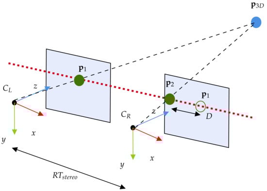
Figure 1.
Stereo vision observation model. A 3D point is reprojected in both cameras. The extrinsic calibration of the stereo pair is defined by the rototranslation .
Let us consider a state vector used for a standard EKF SLAM/odometry approach containing the left camera position and orientation , the velocity , and the list of landmarks represented as a 3D point clouds,
Lets note the vehicle state with:
where a landmark is given in the world frame w (note that the method is not restricted to such a state vector: another representation can be used in a similar way). Given the translation and rotation that define the pose of the left camera in the world frame (),
and:
the intrinsic calibration matrix of the camera (in our case, we supposed without lost of generality that , but one could use two different values for a bi-monocular approach). The 3D point can be reprojected in the left camera frame by using the standard camera projection matrix,
In a similar way, we can obtain the reprojection of the landmark in the right camera, by using its pose in the world frame: and . Thus, we have,
Then, one can note that,
and that the displacement from one camera to the other one is given by the extrinsic calibration step such as,
with and ( for stereo), so we have in our case:
Finally, for each observed 3D point of the environment by both cameras of the stereo pair, we obtain the 4D observation vector given by the true observation model,
where and are strongly dependent on the calibration value of the stereo pair used in .
Note that, in the case where the stereo baseline middle point is taken as the body frame reference, both left and right 2D detection are impacted by the calibration parameters, but the exact same estimation technique can be used.
We defined in the case of a stereo camera approach the observation function and the measurement model parameters that impact this model. The main idea is to use the LCEKF described in Section 3.1 in order to mitigate the errors coming from this mismatched observation model .
3.3. LCEKF Customization for Stereo-Based Visual Navigation
In order to be able to apply the LCEKF approach, the prerequisite is to process the Jacobian of the observation function with respect to parameters , that is to calculate the Jacobians of (23) and (24). However, a direct application of the algorithm proposed in [29] failed. Indeed, when considering SLAM approaches, the constraint on the update step is not sufficient. Each time a new object is seen, a new landmark has to be initialized and set into the map, making the state vector of a dynamic size. This step makes use of a classical two-view triangulation function, which is also dependent on the mismatched parameters . A new 3D point is initialized from two 2D observations and in such a way that,
The landmark 3D world coordinates are processed through as follows. Let and be the homogeneous coordinates of the left and right 2D detection. Let and be the coordinates of the reprojection of the landmark 3D point into the left and right camera image planes,
We need to minimize the reprojection error , , which is equivalent to having and collinear, so the cross-product should be:
By rewriting (32) with a matrix function of as , we can easily process the landmark coordinates by using the mismatched model (indeed, is a function of ). Note that its covariance can also be easily processed at this step.
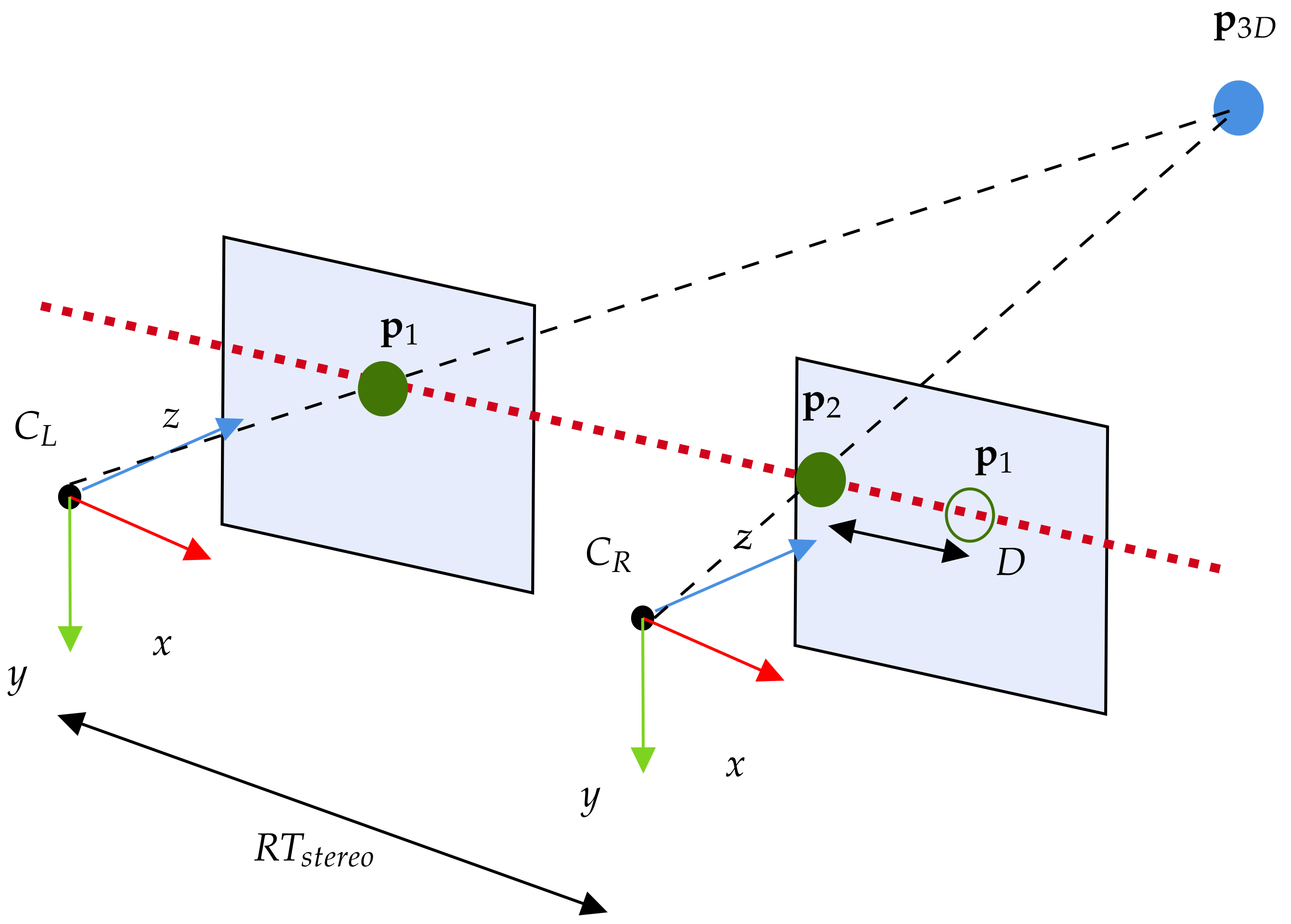
Classical SLAM approaches would append the map with this new landmark such as presented in Figure 2a. Nevertheless, in the LCEKF SLAM framework, a new landmark cannot be directly included in the map with its covariance as it would be calculated with mismatched parameters. We observed that proceeding that way made the LCEKF diverge. We had to take into account the errors of the calibration parameters at the mapping step in the following way. First, we initialized a new landmark in the map state vector with its calculated pose associated with a huge covariance (see Figure 2b).
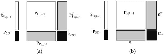
Figure 2.
(a) represents the classical map state appended upon landmark initialization. The appended parts correspond to the landmark’s mean and covariance (black) and the cross-variances between the landmark and the rest of the map (gray). (b) represents the appended solution used followed by an update under constraints.
Then, we classically extended the state vector and the state covariance matrix with this new landmark. The final step would be to perform an update of this new landmark by using the observations and in order to correct its pose and covariance. We can see that such an update makes use of the same observation function (28) as for a classical update step so the constraint can be applied in the same way for the mapping and the update step. We had to calculate the Jacobian of with reference to the state vector including the new landmark and proceed with the constraint as explained before. Nevertheless, by performing such an update at this step, we would only have four observations (two for and two for ), but we require six degrees of freedom to constrain the six parameters of .
Therefore, we postponed the update step of the landmark pose and covariance and processed it simultaneously with the classical LCEKF update step. The advantages were: first, we obtained more degrees of freedom to apply the constraints as we should have more than one landmark observed; second, we did not require processing the Jacobians of twice. Finally, in the case that we had to initialize more than one new landmark at the same time, we also ensured had enough degrees of freedom to fully apply the constraints.
4. Experiments
In order to evaluate our proposed LCEKF-based robust visual navigation, we made a comparison with:
- A standard EKF-based navigation that supposes the given calibration parameters to be good (denoted EKF);
- A standard EKF-based navigation that contains the 6 parameters of in its state vector such that the recalibration is performed on-line (denoted EKFfull).
In order to obtain a fair comparison, we conducted the experiment in a simulated environment where the 2D detection matching was perfectly known, to get rid of outliers that could impact the solution. Indeed, it is well known that in Kalman filtering approaches, the data association problem can quickly cause filter divergence. We chose to validate our approach in a perfectly known detection/matching context in order to only focus on the impact of miscalibration in such a perfect case.
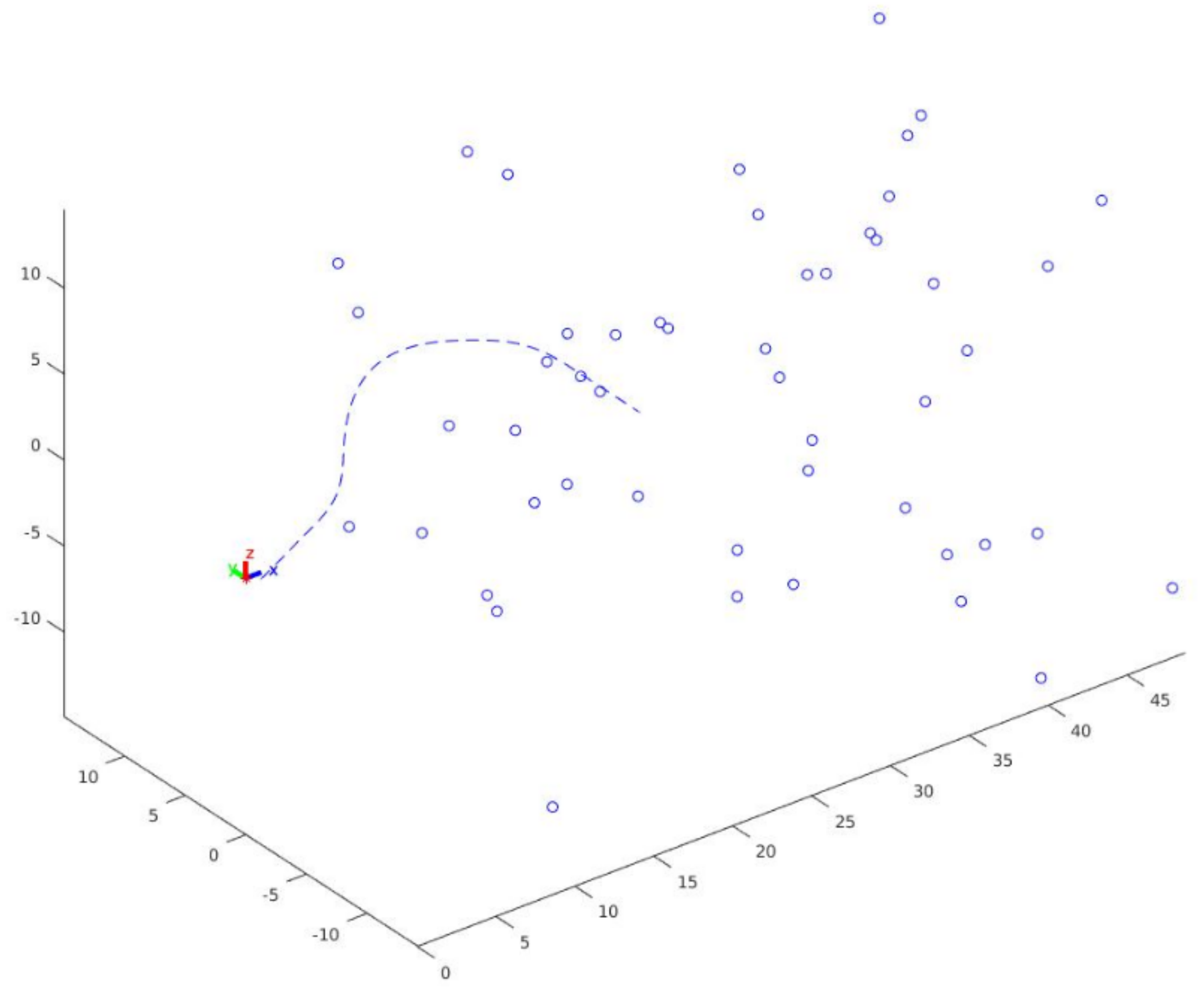
Considering the 3D simulated trajectory, as the main objective of this work was to apply the theory to a simplified case and to prove the feasibility of our method, the simulated world was simply composed of randomly generated 3D points around the trajectory. An example of the studied case is provided in Figure 3.
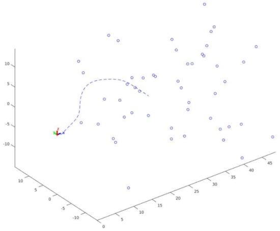
Figure 3.
Simulated trajectory. This example represents one of the studied 6D trajectories generated along a spline with its associated random 3D point cloud.
Moreover, we performed 100 Monte Carlo runs, where for each trial, the three approaches ran with the same noise realization. Furthermore, different noise amplitudes were tested to see the limits of each solution.
We tested the three solutions (EKF, LCEKF, and EKFfull) in a full EKF-SLAM approach in which the map was unknown and built iteratively. This represents the case of an exploration rover where the environment is unknown and needs to be mapped. Such an analysis is conducted in Section 4.3.
4.1. State/Measurement Models
For the prediction step of our Kalman filtering approaches, we tested two evolution models: a constant velocity model and one based on the IMU. Both models showed that the LCEKF was equivalent to or better than the EKFfull. We present both the classical visual-IMU approach and the visual-only approach with a constant velocity assumption.
The simulated inertial measurement unit (IMU) provided acceleration and angular velocity . Such data were expressed first in the camera frame (the body B to navigation N frame conversion was at this step needed and made use of bias and gravity). To use the IMU, we augmented the state vector with the bias estimate of the accelerometer and gyrometer . We integrated the data in a very standard way with constant bias,
Considering the observation/measurement model, we used the one defined in Section 3.2. The prediction was performed at a frame rate of 100 Hz, while the observations came at 20 Hz. The maximal simulated field of view of the camera was fixed to a maximum of 100 m, and images were simulated at a VGA resolution of 640 × 480 with the intrinsic calibration matrix :
4.2. Noises and Miscalibration/Decalibration Types
In order to evaluate the performance and limits of each method, we propose to add some noise to the calibration parameters . We explored five cases for :
- (i)
- Reference case: ;
- (ii)
- Constant noise: . This represents the use of the wrong initial calibration, but with no stress during the experiment;
- (iii)
- Sinusoidal noise: . This case represents for example the day/night thermal constraint encountered for planetary exploration rovers;
- (iv)
- Discontinuous noise: . This case represents a chock or accident encountered while navigating ( can be a combination of Heaviside functions);
- (v)
- Periodic noise: ; This case simulated a strong vibration of the system for a non-perfectly rigid stereo system ( is a periodic square wave).
For all the experiments, noise was added to the inputs of the system according to the covariances defined hereafter:
- For the IMU: ; ;
- For the 2D detections: .
with
the time between two prediction and the covariance of the measurement. The calibration parameters are defined with a perfect stereo configuration and a baseline of 2 m:
Different calibration errors were tested. We arbitrarily chose to present results with a decalibration involving a error on the baseline. In the results below, was processed with:
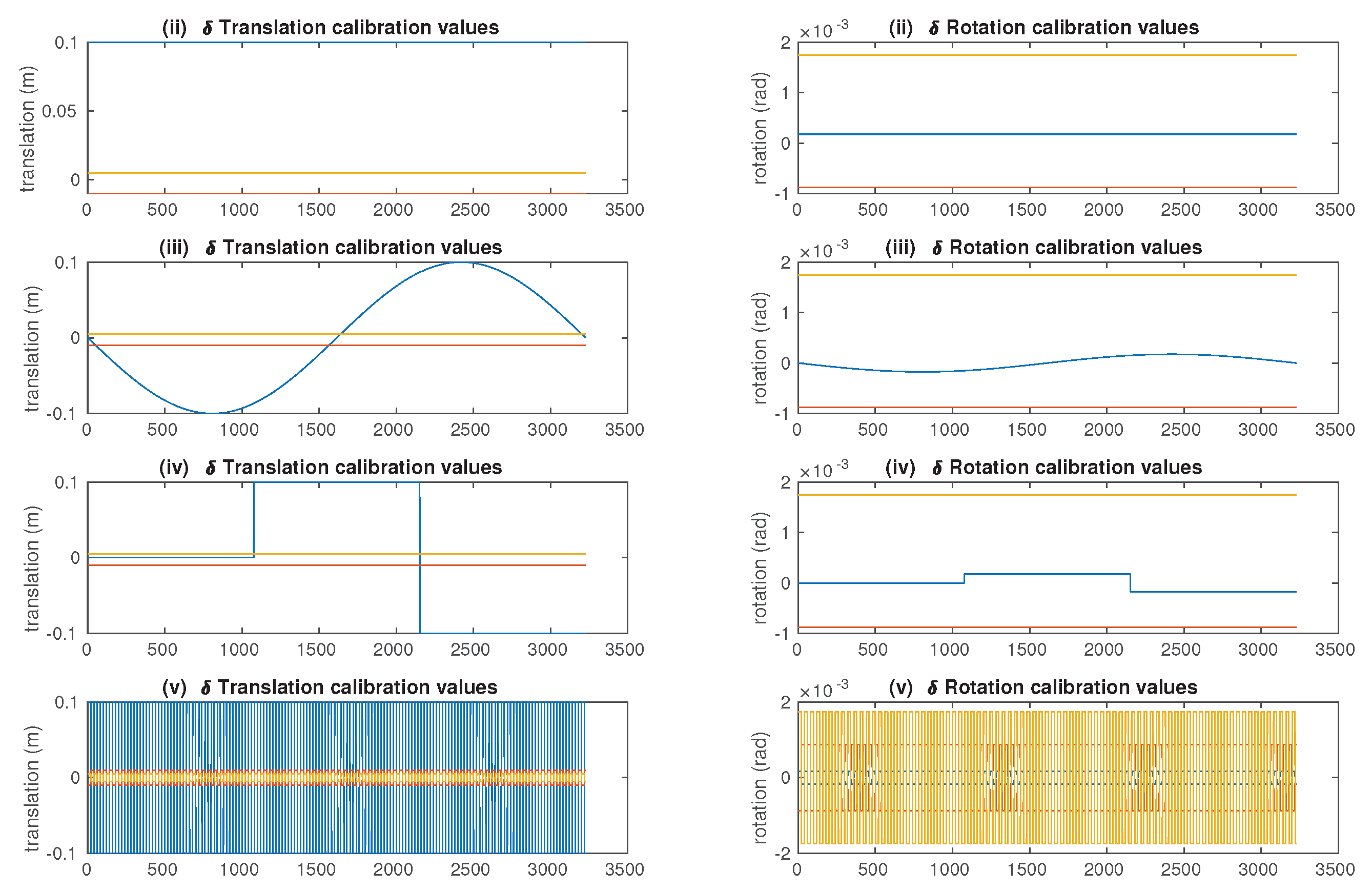
The ground truth calibration error values during each experiment are presented in Figure 4.
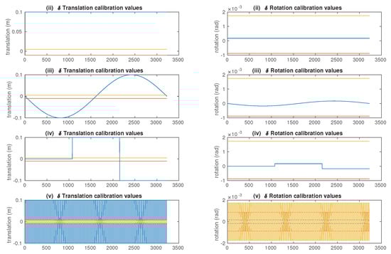
Figure 4.
Ground truth error calibration value for the different experiments. Major effects of decalibration noise are applied on the translation (the baseline) and on the rotation (rotation around the baseline axis). Blue, red, and yellow are respectively the values for , , and and , , and .
4.3. SLAM Experiment with IMU
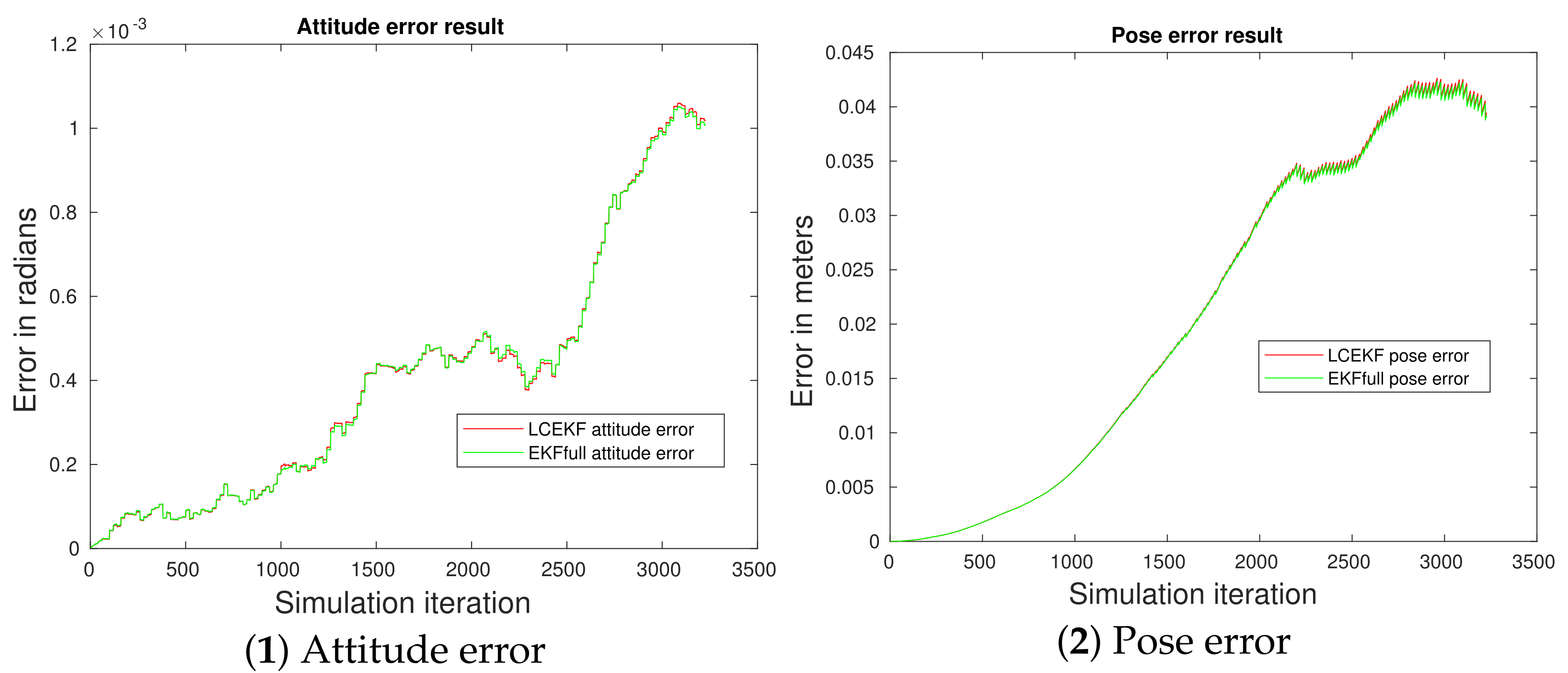
4.3.1. Reference Case Comparison (i)
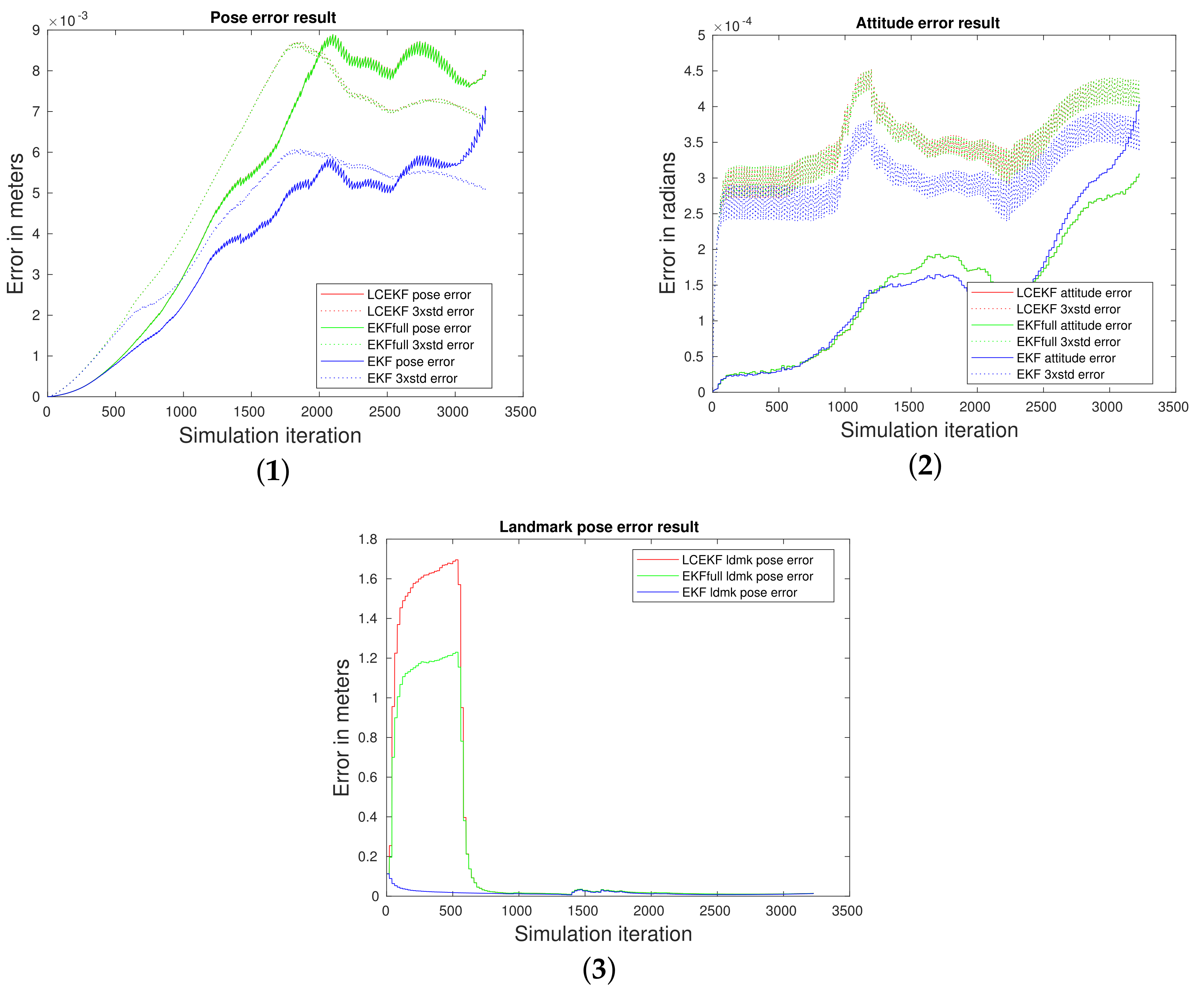
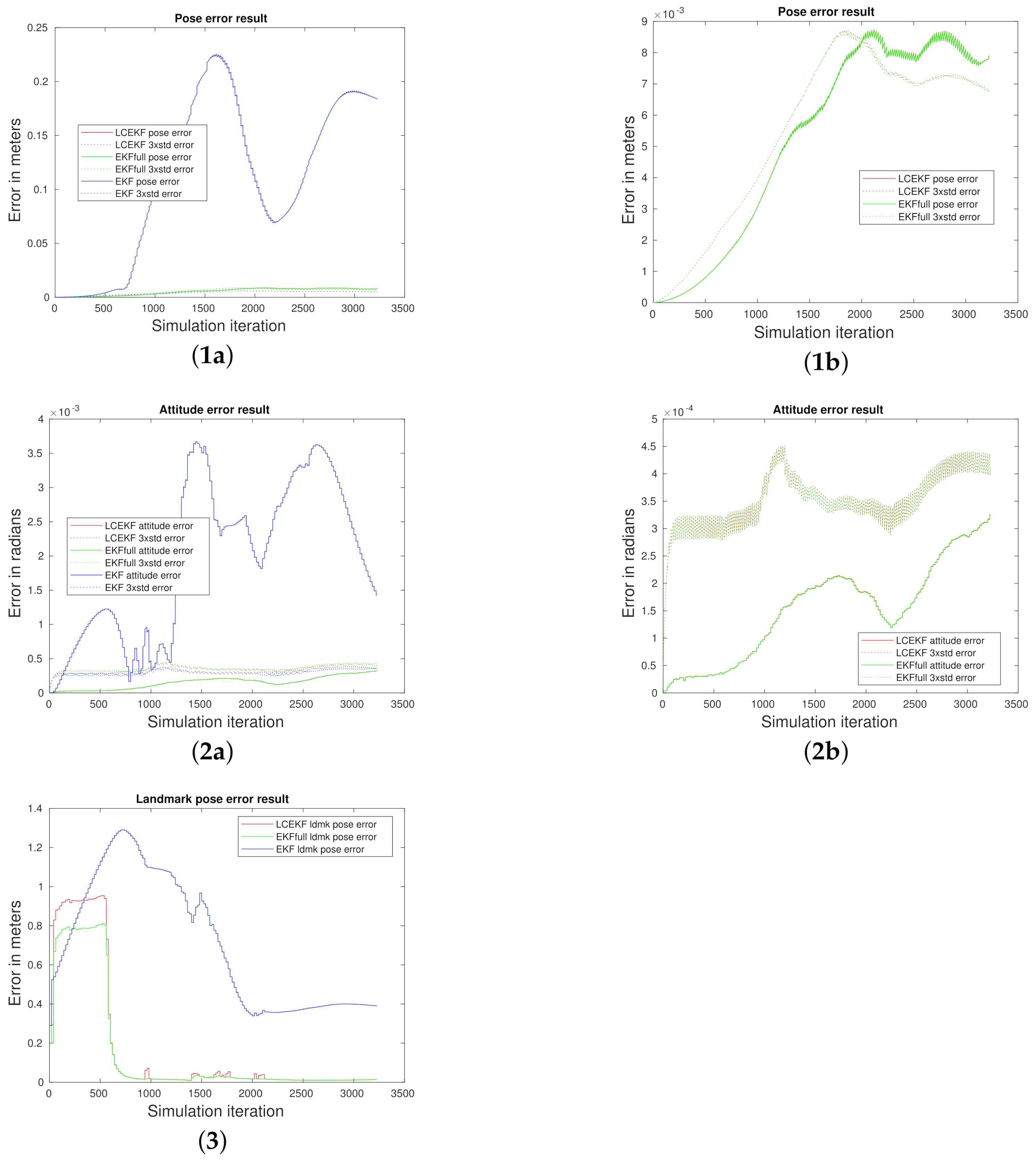
The objective of this experiment was to test the efficiency of the EKF in a nominal case, as well as to explore the impact of constraints for the LCEKF and additional parameters to estimate for the EKFfull. Localization (including rotation and position) and mapping (landmarks poses) errors are presented in Figure 5. It can be clearly seen that both the LCEKF and EKFfull provided the same localization results. Considering the mapping, the EKFfull showed better initialization of the landmarks, but the same convergence. As expected, the EKF with perfect knowledge of the calibration outperformed the two extended approaches as the EKFfull compensates observation errors and noise by changing the calibration parameters, and the LCEKF consumes degrees of freedom by fixing constraints on the Kalman gain.
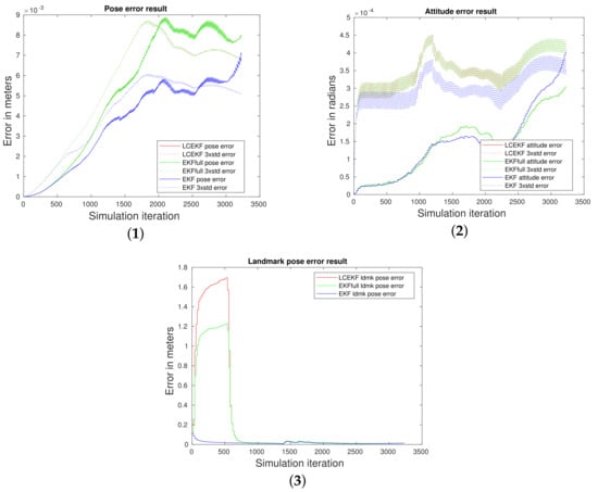
Figure 5.
SLAM without noise (Case i): methods’ comparison. (1) and (2) represent respectively the MSE of the pose and attitude estimation over 100 executions. Full lines are the mean of the estimation, and dotted line represent the 3 sigma values. (3) represents the MSE of the landmark convergence during the simulation.
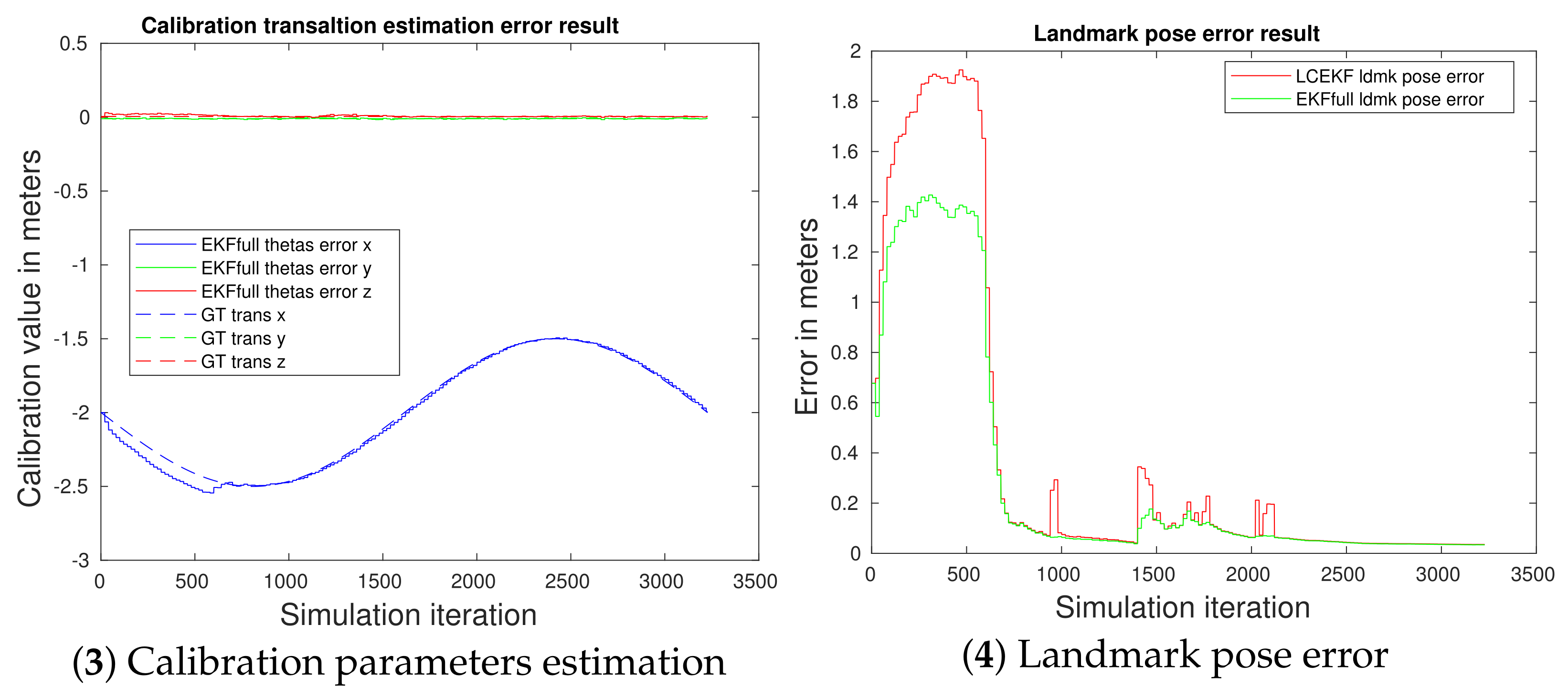
4.3.2. Noisy Cases (ii), (iii), and (iv)
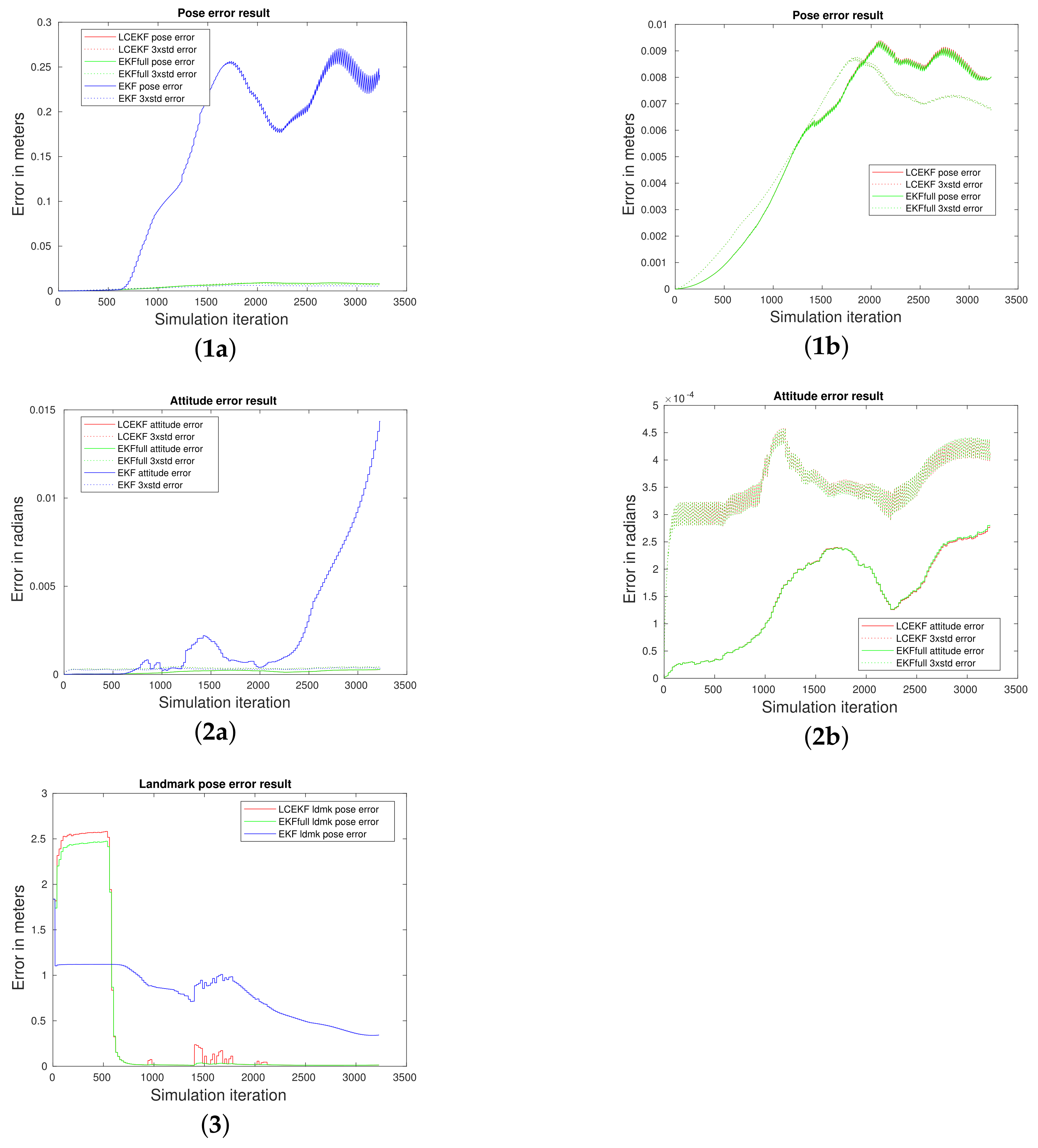
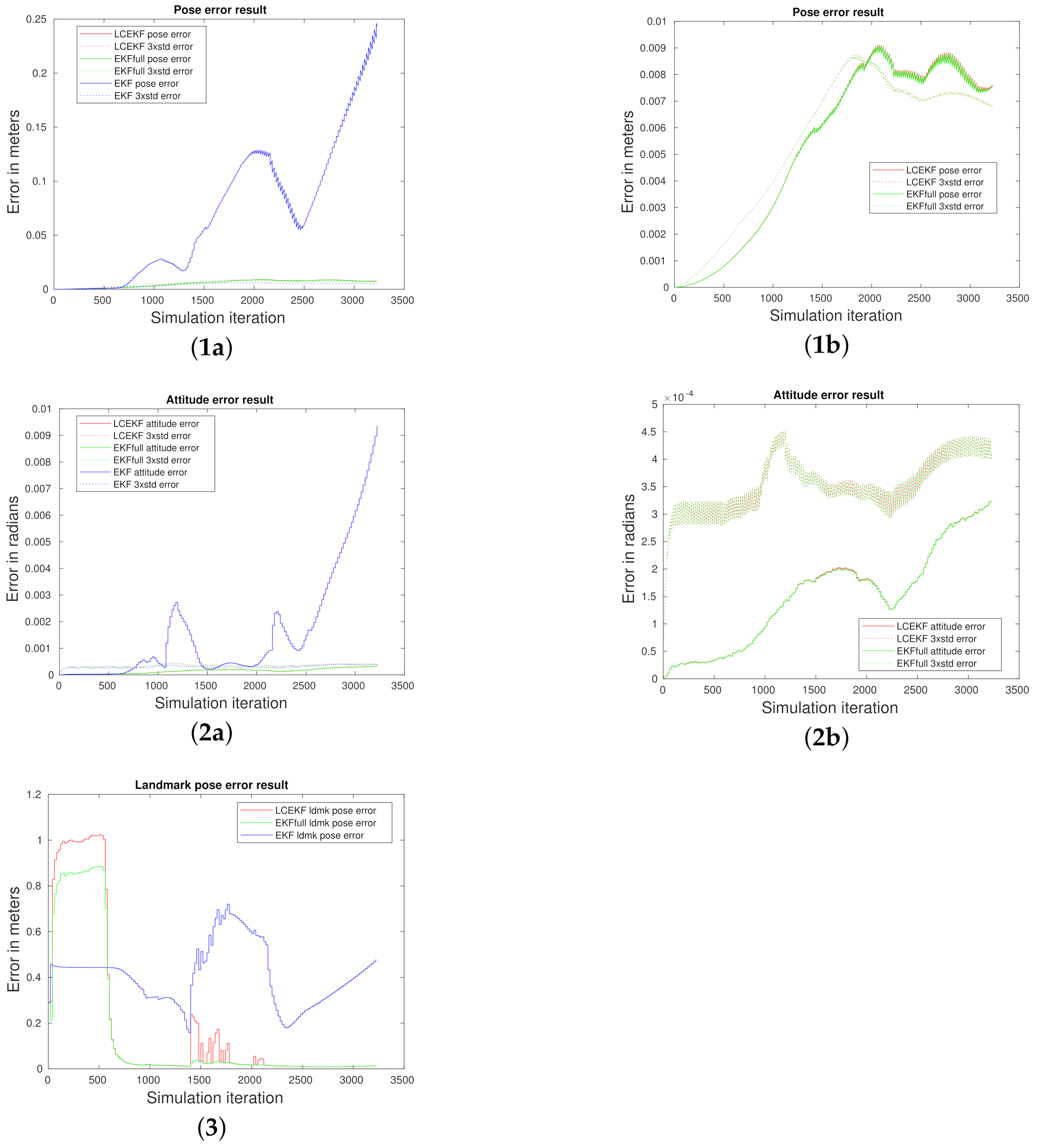
The results are provided in Figure 6 for the constant noise Case (ii), in Figure 7 for sinusoidal noise (iii), and in Figure 8 for discontinuous noise (iv). For all these tests with a mismatched model, it is clear that the standard EKF diverged and did not provide any good results. An interesting thing to note is that both the LCEKF and EKFfull provided the same results, while the first one did not estimate the calibration on-the-fly (both the red curves and green curves are overlapping). Moreover, whatever the noise applied on the calibration, the results were quite equivalent. The main difference can be observed on the mapping results. We can see that the landmark convergence was good for both techniques, but the initialization was a little bit better for the EKFfull. This can be easily explained by the fact that the LCEKF initialization makes use of constraints on the mismatched model and not of the closest estimation of the true model. Nevertheless, the convergence after multiple observations was as good as the one of the EKFfull.
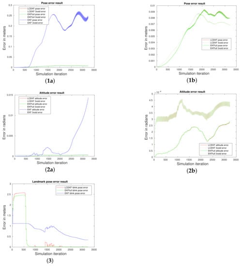
Figure 6.
SLAM with constant noise (Case ii): methods’ comparison. Figures (1a) and (2a) represent the MSE of the pose and attitude estimation over 100 executions for the three methods. As the EKF results hide the two other, the same results without the EKF are presented in Figures (1b) and (2b). Full lines are the mean of the estimation, and dotted lines represent the 3 sigma value. Figure (3) represents the MSE of the landmark convergence during the simulation.
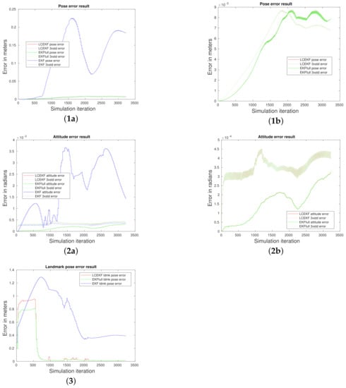
Figure 7.
SLAM with sinusoidal noise (Case iii): methods’ comparison. Figures (1a) and (2a) represent the MSE of the pose and attitude estimation over 100 executions for the three methods. As the EKF results hide the two other, the same results without the EKF are presented in Figures (1b) and (2b). Full lines are the mean of the estimation, and dot lines represent the 3 sigma value. Figure (3) represents the MSE of the landmark convergence during the simulation.
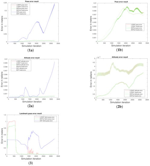
Figure 8.
SLAM with discontinuous noise (Case iv): methods’ comparison. Figures (1a) and (2a) represent the MSE of the pose and attitude estimation over 100 executions for the three methods. As the EKF results hide the two other, the same results without the EKF are presented in figures (1b) and (2b). Full lines are the mean of the estimation, and dotted lines represent the 3 sigma value. Figure (3) represents the MSE of the landmark convergence during the simulation.
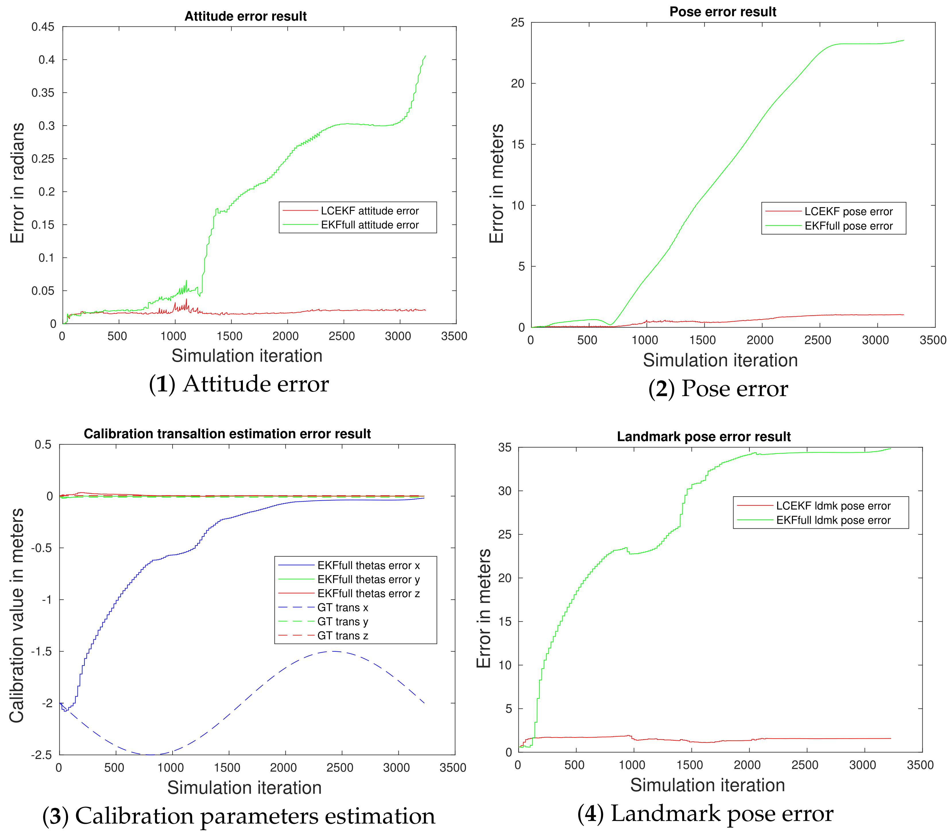
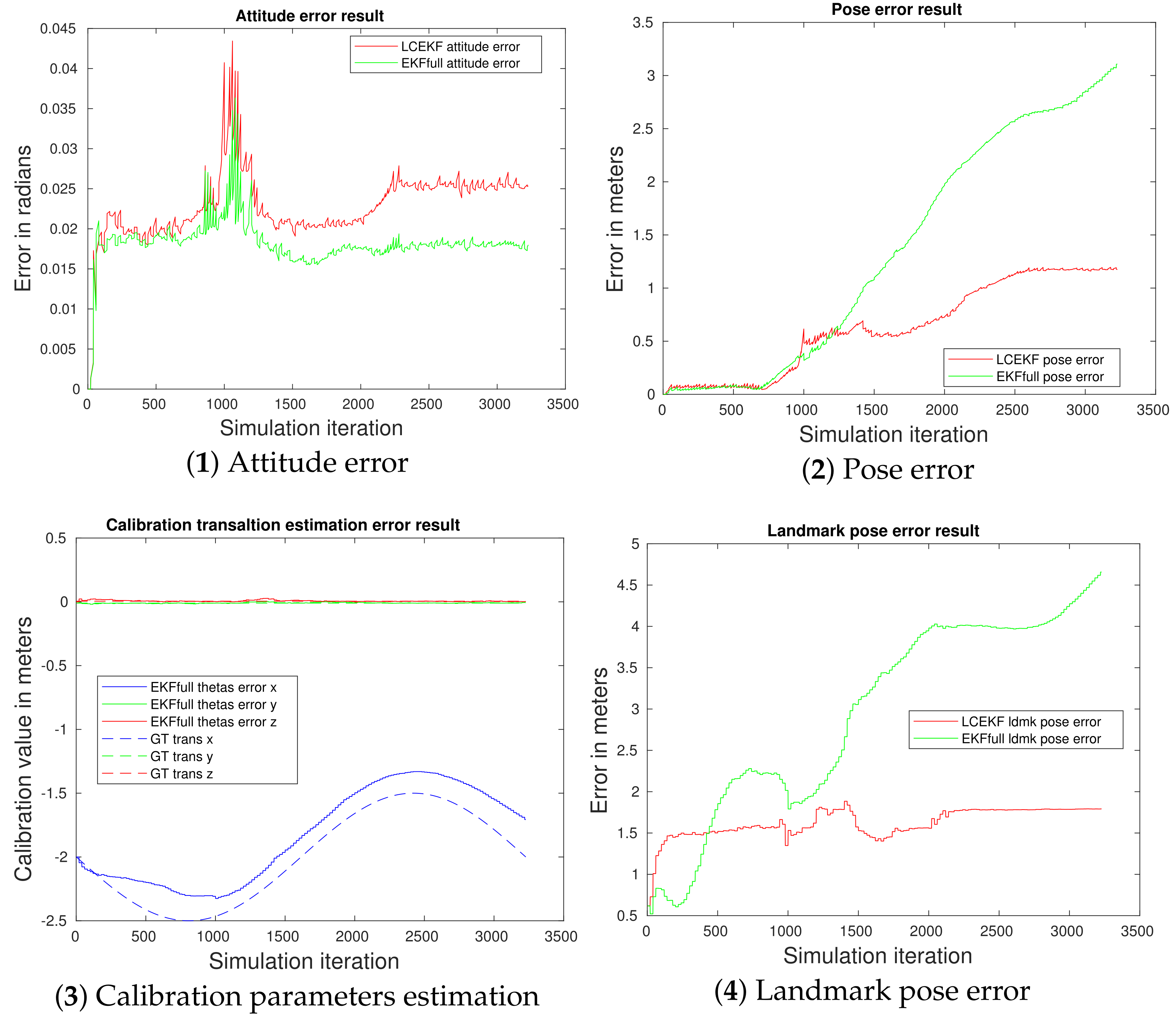
4.3.3. Periodic Noise Case (v)
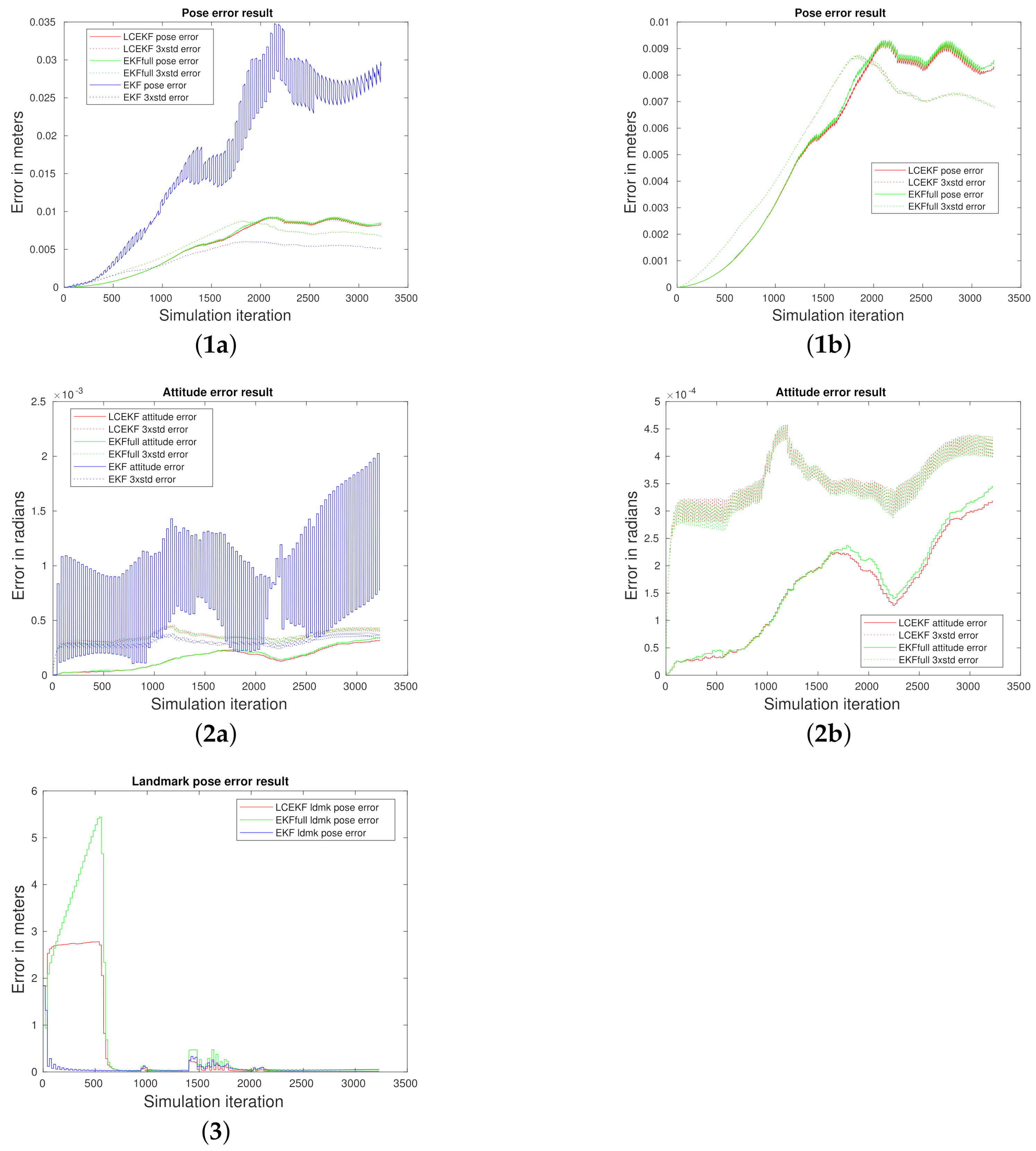
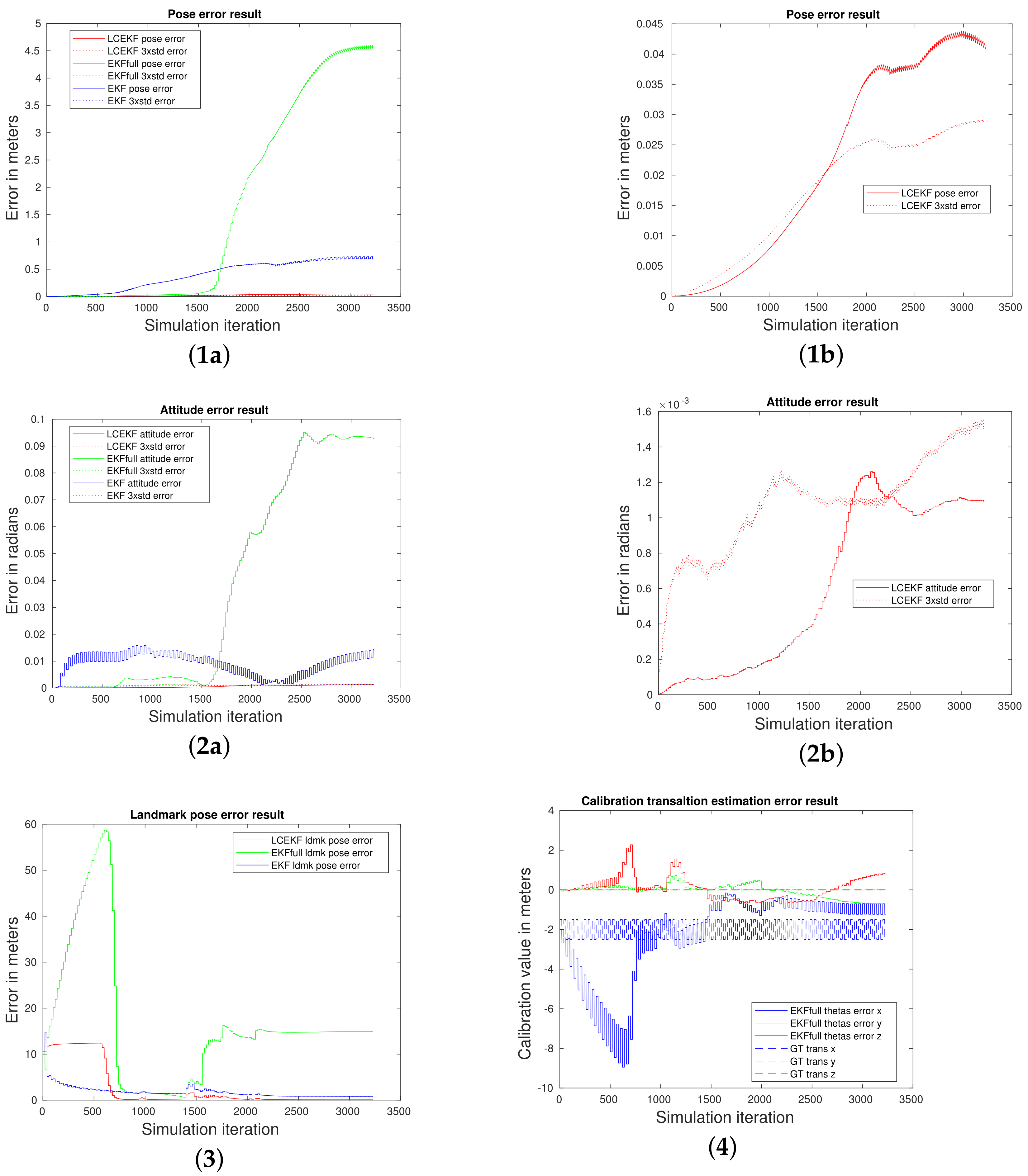
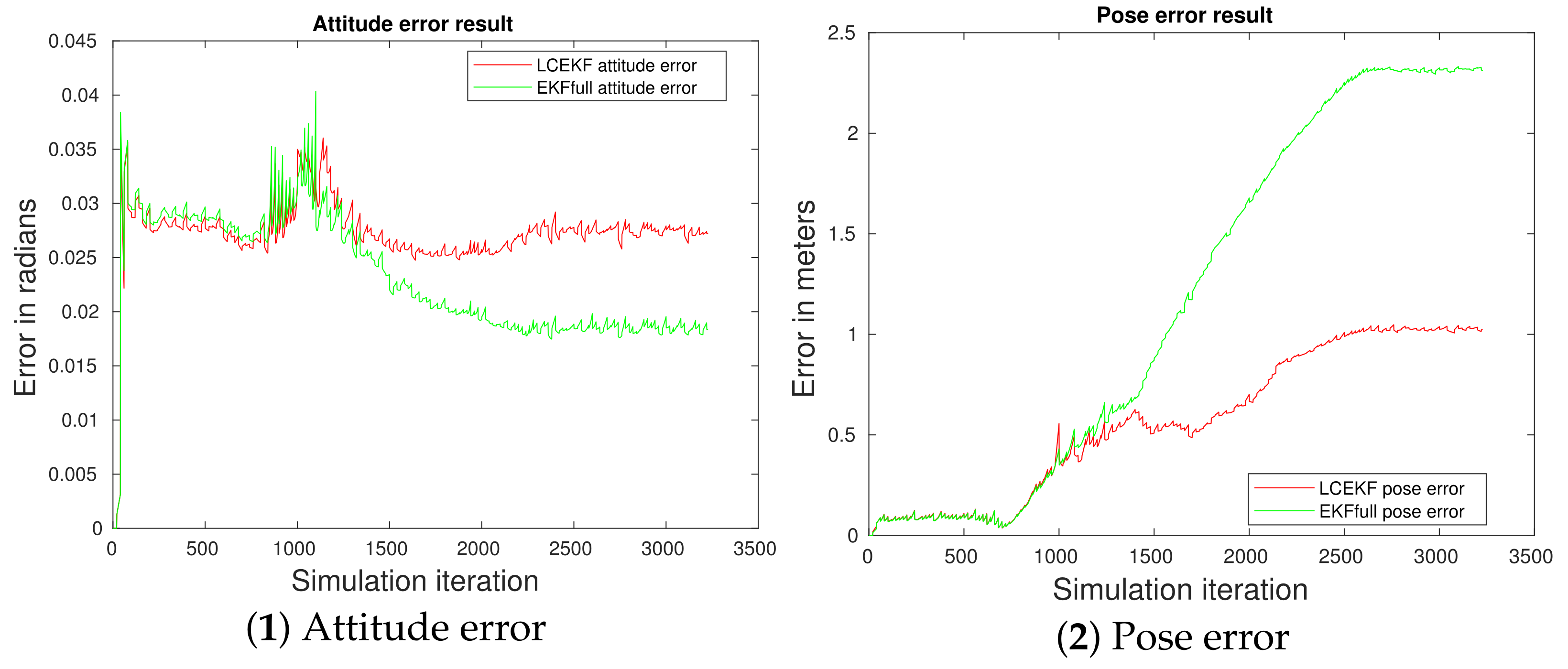
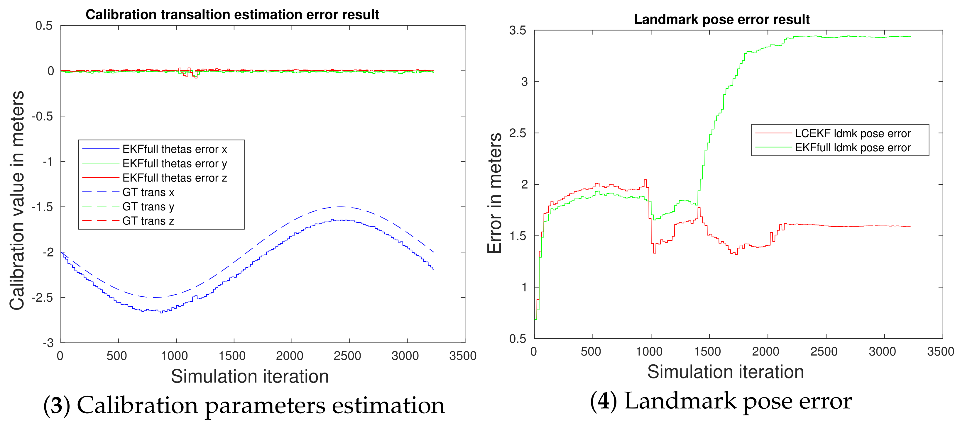
This last case is interesting as we can see a difference between both the LCEKF and EKFfull. Localization and mapping results are provided in Figure 9. As the vibration was fast and strong, the estimation of calibration parameters was no longer always fast enough to fit the true model. In such a case, the LCEKF showed quite better performances. If the noise was very strong as in Figure 10 (0.5 m on the baseline), the EKFfull diverged as it worked with a changing, but still miscalibrated system. In this experiment:
As the noise was centered and periodic, it could be observed that the EKF performed better than the EKFfull. The divergence could be observed when the estimation of the calibration was too slow. In such extreme cases, the LCEKF clearly outperformed both the EKF and the EKFfull showing the efficiency of the proposed approach, even in the presence of very big disturbances.
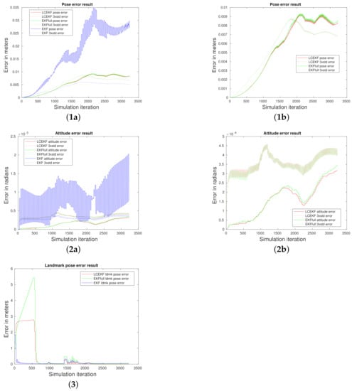
Figure 9.
SLAM with periodic noise (Case v): methods’ comparison. Figures (1a) and (2a) represent the MSE of the pose and attitude estimation over 100 executions for the three methods. As the EKF results hide the two other, the same results without the EKF are presented in Figures (1b) and (2b). Full lines are the mean of the estimation, and dotted line represent the 3 sigma value. Figure (3) represents the MSE of the landmark convergence during the simulation.
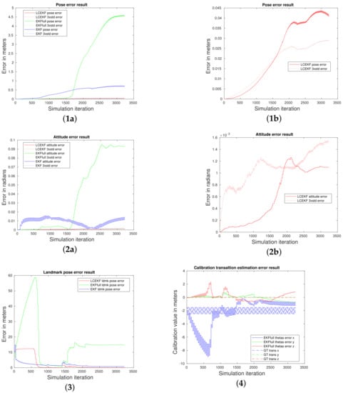
Figure 10.
SLAM with high amplitude periodic noise (Case v): methods’ comparison. Figures (1a) and (2a) represent the MSE of the pose and attitude estimation over 100 executions for the three methods. The LCEKF results without the EKF and EKFfull are presented in Figures (1b) and (2b). Full lines are the mean of the estimation, and dotted lines represent the 3 sigma value. Figure (3) represents the MSE of the landmark convergence during the simulation. Figure (4) shows the EKFfull calibration parameters’ estimation.
4.4. SLAM Experiment Comparison with and without the IMU
In order to prove that the stereo miscalibration compensation was not dependent on the IMU measurements, a comparison with and without the IMU is provided in this section. In both cases, the LCEKF was able to restrain the drift, but also to maintain the scale. Indeed, in classical EKF or bundle-adjustment (BA)-based SLAM, the scale is mainly obtained thanks to the baseline (and IMU). In our case, due to the constraints, the scale was first initialized by the supposed known baseline, but the Kalman gain was then modified with the linear constraints in order to fit the observations. As a result, the scale did not drift.
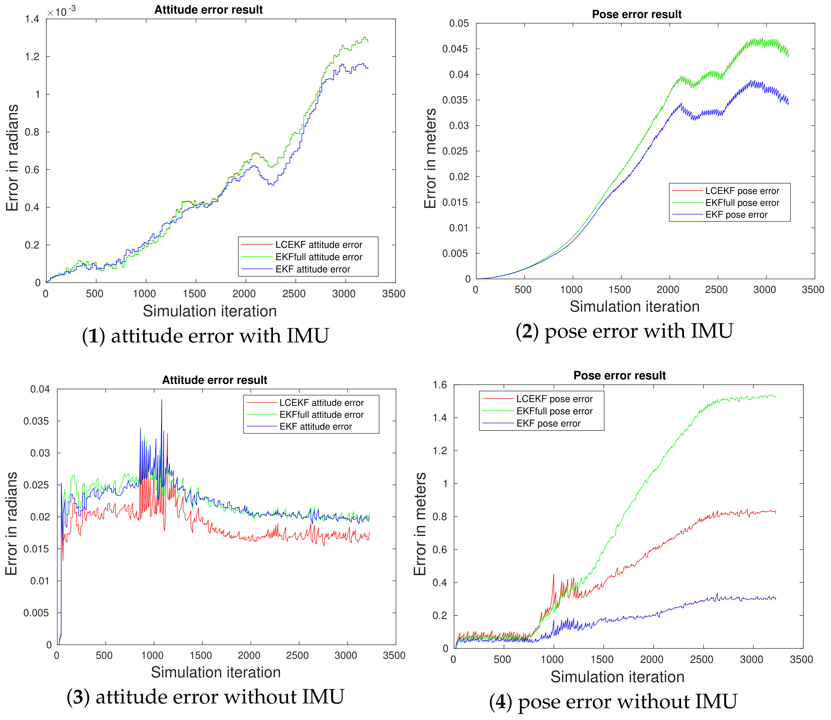
The results for the different noises (i) to (v) with and without the IMU are provided in Figure 11, Figure 12, Figure 13 and Figure 14. As can be seen from the experiments, the LCEKF was for each case more robust than the EKFfull. While removing the IMU, the scale factor of the environment could only be obtained from the stereovision process. If the calibration is not well known, this scale factor will be wrong. In the case of LCEKF, as the observations were constraints, the scale factor was forced to fit the constraints over the observation function. As a result, even if the IMU made the estimation more accurate, it was not mandatory to correct this bias coming from miscalibration.

Figure 11.
SLAM with no noise (Case i): methods’ comparison. Figures (1) and (2) represent the MSE of the pose and attitude estimation over 10 executions for the three methods while using the IMU for prediction. All the methods performed in the same way. Figures (3) and (4) represent the MSE of the pose and attitude estimation over 10 executions for the three methods while using a constant velocity model for prediction (no proprioceptive sensor). It can be seen that without the use of the IMU, both the LCEKF and EKFfull had a positioning error that increased over time (classical observed drift). Nevertheless, the LCEKF is more robust.
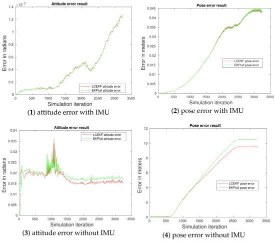
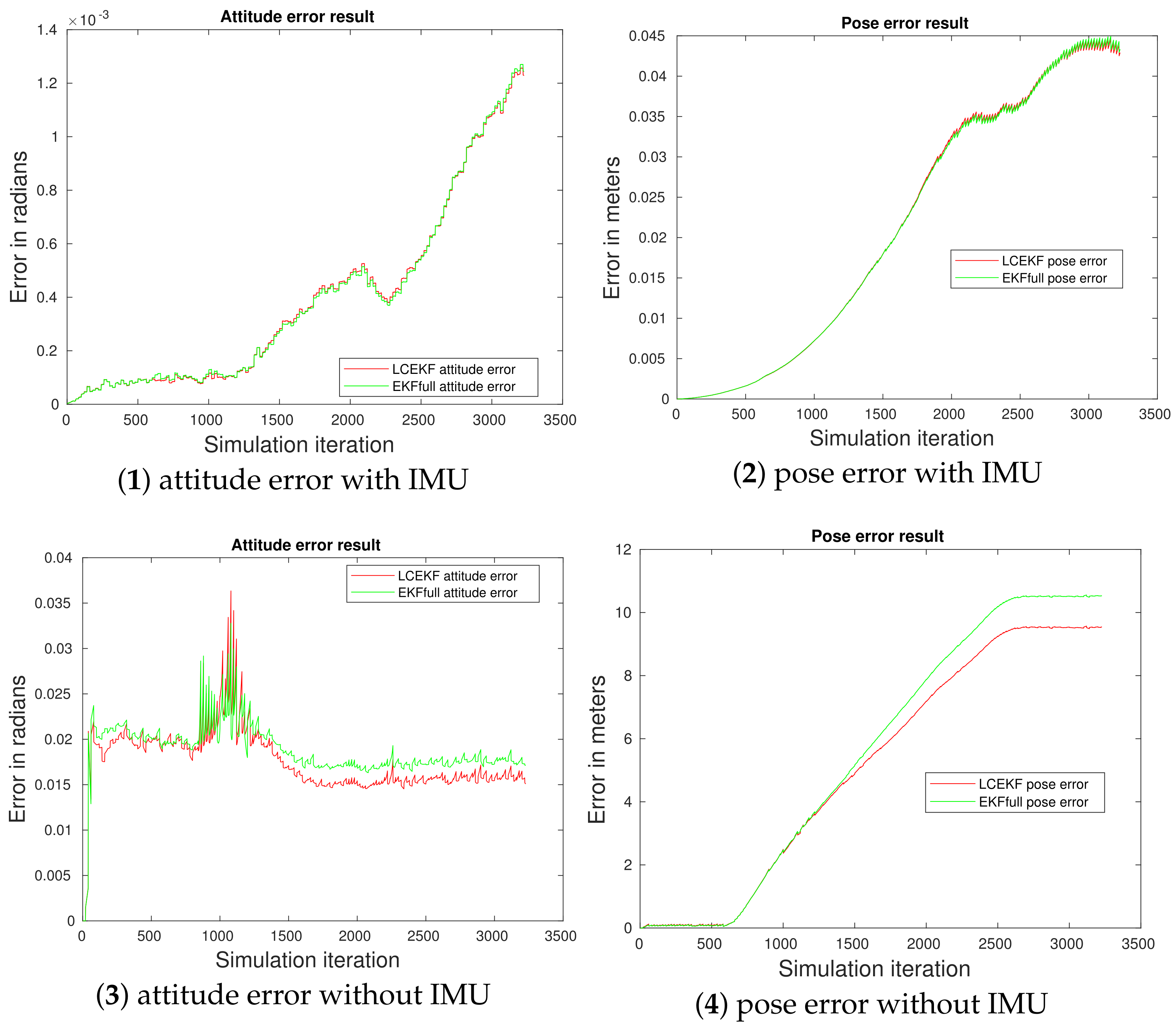
Figure 12.
SLAM with constant noise (Case ii): methods’ comparison. Figures (1) and (2) represent the MSE of the pose and attitude estimation over 10 executions for the three methods while using the IMU for prediction. All the methods performed in the same way. Figures (3) and (4) represent the MSE of the pose and attitude estimation over 10 executions for the three methods while using a constant velocity model for prediction (no proprioceptive sensor). It can be seen that without the use of the IMU, both the LCEKF and EKFfull had a positioning error that increased over time (classical observed drift). Nevertheless, the LCEKF is more robust.
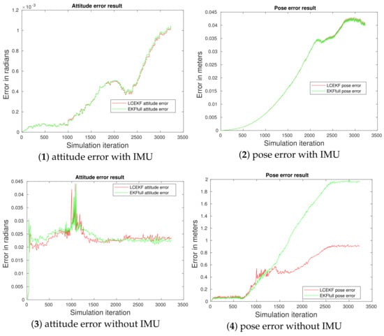
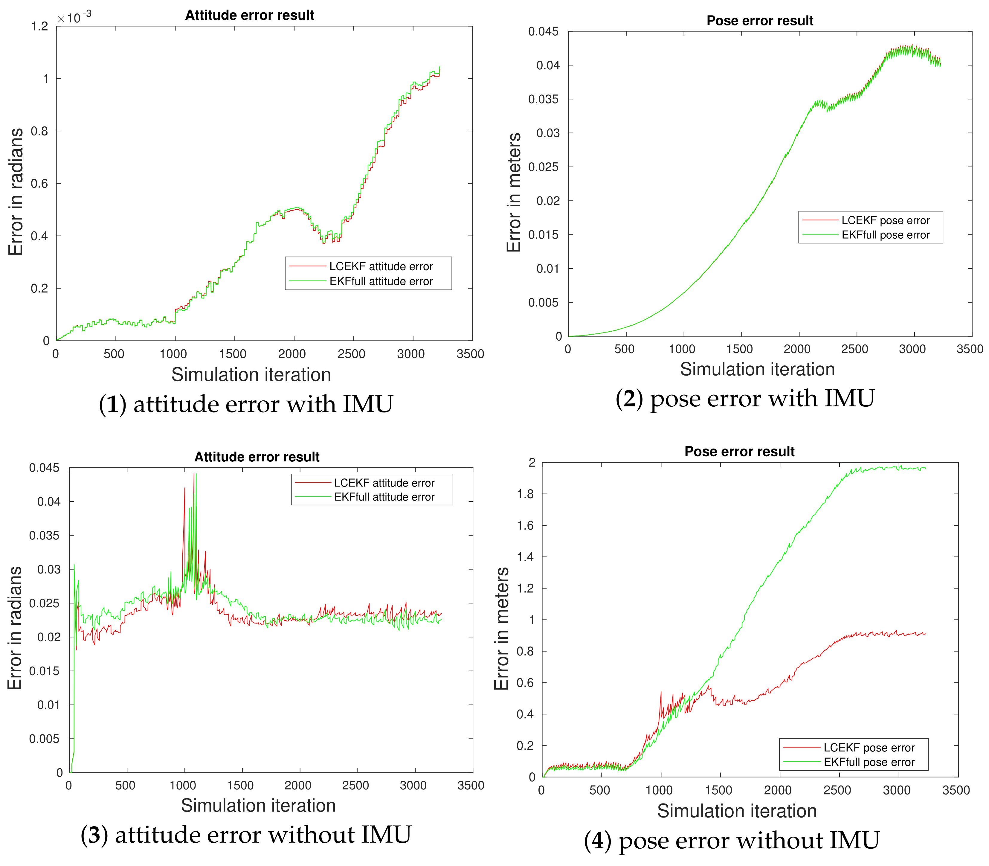
Figure 13.
SLAM with chock noise (Case iii): methods’ comparison. Figures (1) and (2) represent the MSE of the pose and attitude estimation over 10 executions for the three methods while using the IMU for prediction. All the methods performed in the same way. Figures (3) and (4) represent the MSE of the pose and attitude estimation over 10 executions for the three methods while using a constant velocity model for prediction (no proprioceptive sensor). It can be seen that without the use of the IMU, both the LCEKF and EKFfull had a positioning error that increased over time (classical observed drift). Nevertheless, the LCEKF is more robust.

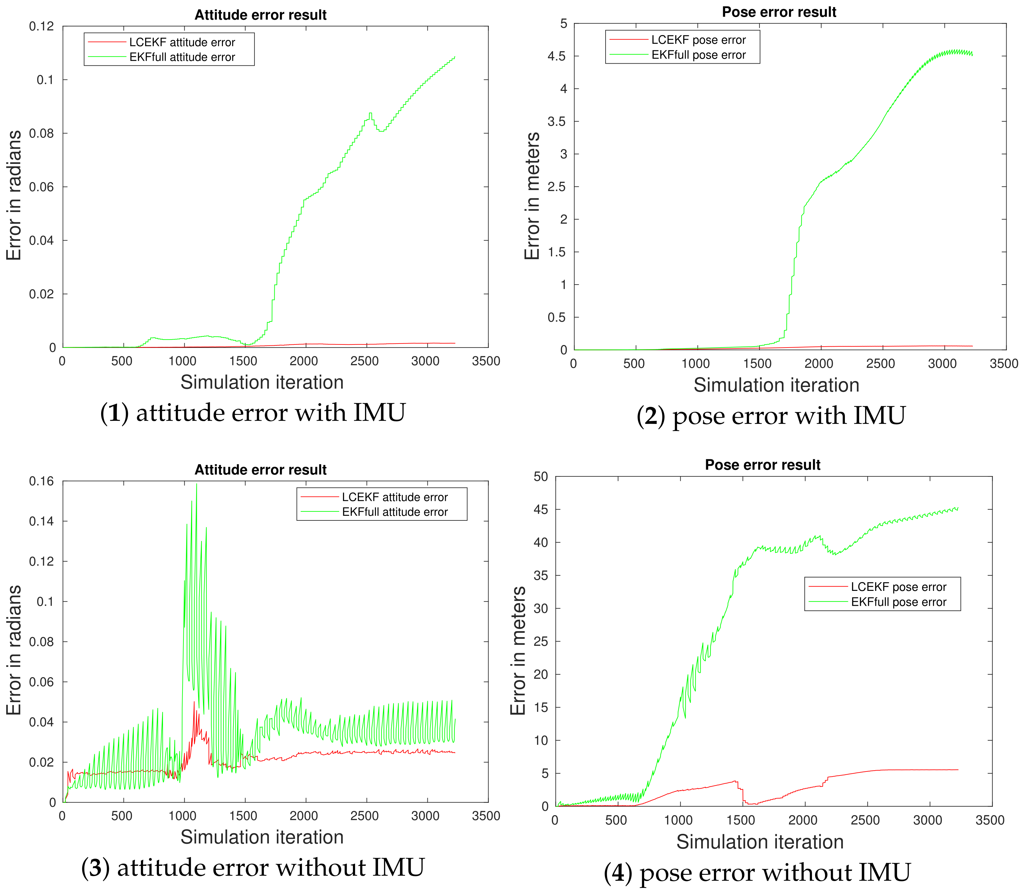
Figure 14.
SLAM with periodic square noise: methods’ comparison. Figures (1) and (2) represent the MSE of the pose and attitude estimation over 10 executions for the two methods while using the IMU for prediction. Figures (3) and (4) represent the MSE of the pose and attitude estimation over 10 executions for the two methods while using a constant velocity model for prediction (no proprioceptive sensor). It can be clearly seen that the EKFfull diverged in both case.
4.5. On the Influence of Kalman Covariance Initialization for Calibration Parameters
As stated before, the main motivation for this work was to apply a theoretical development to a real application. We proved that we can deal with calibration errors without estimating such parameters. Of course, the theory can also be applied to other parameters, as proven in our previous works (both impacting observation or evolution models). When considering experiment with small miscalibration errors, we showed that the performances were quite equivalent with the LCEKF and EKFfull. Nevertheless, the main drawback of using calibration parameter estimation inside a filter-based approach is that it requires an evolution model for all the uncertain parameters. Such models are quite difficult to estimate, and it is well known that the KF is very sensitive to covariances and noise initialization. In order to show the influence of such parametrization, we performed some additional simulations. The parameters of the experiments are described in Table 1. We performed multiple experiments with different parameters for the required random walk over the calibration parameters (well estimated, no noise consideration, underestimated, and overestimated noises).

Table 1.
Study of the influence of covariances’ and noises’ initialization.
As can be seen with these last simulations (Figure 15, Figure 16, Figure 17 and Figure 18), the EKFfull was very sensitive to the covariances used to predict the uncertain parameters, while the LCEKF was totally independent of such data. This point is a major advantage of using constraints instead of estimating the parameters as such noise conditions are very difficult to estimate in any real experiment.
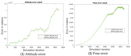
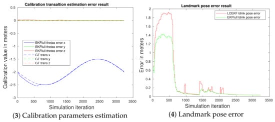
Figure 15.
SLAM without the IMU and smooth sinusoidal noise. With a good random walk for K parameters, the estimation performed properly, making the EKFfull work fine. Note that the LCEKF and EKFfull performed in the same way.
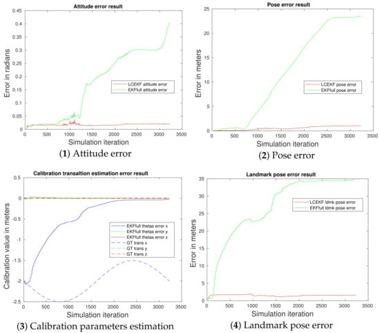
Figure 16.
SLAM without the IMU and smooth sinusoidal noise. Without random walk for K parameters, the estimation was not performed properly, making the EKFfull diverge. Note that there was no impact on the LCEKF as the K parameters were not estimated.
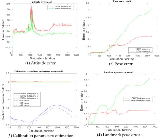
Figure 17.
SLAM without the IMU and smooth sinusoidal noise. With underestimated random walk for K parameters, the estimation was not performed properly, making the EKFfull diverge. Note that there was no impact on the LCEKF as the K calibration parameters were not estimated.
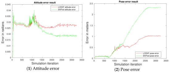
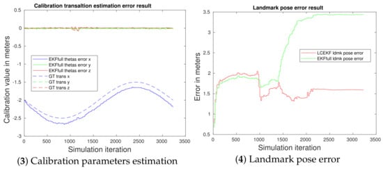
Figure 18.
SLAM without the IMU and smooth sinusoidal noise. With overestimated random walk for K parameters, the estimation was not performed properly, making the EKFfull diverge. Note that there was no impact on the LCEKF as the K calibration parameters were not estimated.
Conclusions
It is interesting to see that, in the case that the model used was perfect, indeed, when we do not have any error on , the standard EKF performed very well, as predicted by the theory, while both the LCEKF and EKFfull had a good, but quite inferior performance. This is easily explainable by the fact that the EKFfull ties to compensate errors and noise from the measurements by changing the calibration parameter, and so, by creating a mismatched model. Regarding the LCEKF, using constraints on the calculation of the gain consumes degrees of freedom for the update step, reducing the achievable performance of the optimal filter.
Considering the case with a mismatched model, it is clear that the standard EKF SLAM diverged whatever the noise shape was, which supports the need for improved solutions in practice. Both the LCEKF and EKFfull maintained almost the same performances for all the experiments. A difference can be noted on the landmark pose error at the start of the trajectory. The LCEKF had a stronger error for the initialization of the landmark. Indeed, by trying to neglect calibration errors, the first initialization under the constraints was much less precise than a direct initialization with estimated calibration (if the estimation was good). This can also be seen when new landmarks were initialized around Iteration 1500. Nevertheless, such landmark error was quickly reduced, and the landmark pose converged to the one of the EKFfull.
This last conclusion was no longer true in the case of periodic noise representing the high vibration of the system. In this case, the estimation of the calibration parameters performed by the EKFfull was not always fast enough to ensure a good calibration over time. On its side, the LCEKF mitigated the noise (even with a very high amplitude) and provided a much better performance.
The last point is the consideration of the random walk for the estimated calibration parameters. Such inline calibration estimation required a good knowledge of the noises. In the case that these parameters are not well estimated, the Kalman Filter approaches are prone to diverge, as shown by our last simulation. Considering the LCEKF, as no noise model was needed, our solution was totally insensitive to such parameters, making the solution well suited for such applications.
5. Conclusions and Future Work
This article proposed a new solution to mitigate the problem of a misspecified model in the case of EKF-based SLAM approaches with two cameras. Our solution used the addition of a linear constraint in the calculation of the Kalman gain in order to match the true measurements to the assumed (mismatched) model. We could observe quasi-similar results with our LCEKF or an EKF in which the calibrations parameters were perfectly estimated. Nevertheless, in the case of extreme perturbation of the parameters or when the covariances of the parameters was not well estimated (as is the case in all real scenarios), the LCEKF clearly outperformed the standard approach. The proposed solution is well fit for robots/vehicles in which the estimation of such calibration parameters is not feasible or not performed (low embedded power, etc.), when the initial calibration for each robot is difficult (huge homogeneous robot fleet), or when the system is submitted to vibration that will impact the calibration in an uncertain way such that the noise covariances cannot be known. As future work, it would be of interest to analyze and extend the exploitation of linear constraints using a Lie group formulation and within the context of an optimization framework to better cope with the system nonlinearities and to be included in current state-of-the-art SLAM approaches.
Author Contributions
Conceptualization, D.V., E.C. and J.V.-V.; methodology, D.V., E.C. and J.V.-V.; software, D.V.; validation, D.V. and E.C.; formal analysis, D.V.; investigation, D.V.; resources, D.V.; data curation, D.V.; writing—original draft preparation, D.V. and G.P.; writing—review and editing, G.P., D.V., E.C. and J.V.-V.; visualization, G.P., D.V., E.C. and J.V.-V.; supervision, E.C.; project administration, E.C.; funding acquisition, E.C. and J.V.-V. All authors have read and agreed to the published version of the manuscript.
Funding
This research was partially supported by the DGA/AID Projects 2019.65.0068.00.470.75.01 and 2021.65.0070.00.470.75.01.
Institutional Review Board Statement
Not applicable.
Informed Consent Statement
Not applicable.
Data Availability Statement
Not applicable.
Conflicts of Interest
The authors declare no conflict of interest.
References
- Szczepanski, M. Online Stereo Camera Calibration on Embedded Systems. Ph.D. Thesis, Université Clermont Auvergne, Clermont-Ferrand, France, 2019. [Google Scholar]
- Blume, H. Towards a Common Software/Hardware Methodology for Future Advanced Driver Assistance Systems; River Publishers: Roma, Italy, 2017. [Google Scholar]
- Longuet-Higgins, H.C. A computer algorithm for reconstructing a scene from two projections. Nature 1981, 293, 133–135. [Google Scholar] [CrossRef]
- Hartley, R. In Defense of the 8-Point Algorithm. IEEE Trans. Pattern Anal. Mach. Intell. 1997, 19, 580–593. [Google Scholar] [CrossRef] [Green Version]
- Nistér, D. An efficient solution to the five-point relative pose problem. IEEE Trans. Pattern Anal. Mach. Intell. 2004, 26, 756–770. [Google Scholar] [CrossRef] [PubMed]
- Zhang, Z.; Luong, Q.T.; Faugeras, O. Motion of an uncalibrated stereo rig: Self-calibration and metric reconstruction. IEEE Trans. Robot. Autom. 1996, 12, 103–113. [Google Scholar] [CrossRef]
- Zhang, Z. A flexible new technique for camera calibration. IEEE Trans. Pattern Anal. Mach. Intell. 2000, 22, 1330–1334. [Google Scholar] [CrossRef] [Green Version]
- Takahashi, H.; Tomita, F. Self-Calibration of Stereo Cameras; ICCV: Vienna, Austria, 1988. [Google Scholar]
- Sun, P.; Lu, N.G.; Dong, M.L.; Yan, B.X.; Wang, J. Simultaneous all-parameters calibration and assessment of a stereo camera pair using a scale bar. Sensors 2018, 18, 3964. [Google Scholar] [CrossRef] [PubMed] [Green Version]
- Dang, T.; Hoffmann, C. Stereo calibration in vehicles. In Proceedings of the IEEE Intelligent Vehicles Symposium, Parma, Italy, 14–17 June 2004. [Google Scholar]
- Dang, T.; Hoffmann, C.; Stiller, C. Self-calibration for active automotive stereo vision. In Proceedings of the IEEE Intelligent Vehicles Symposium, Meguro-Ku, Japan, 13–15 June 2006. [Google Scholar]
- Dang, T.; Hoffmann, C.; Stiller, C. Continuous Stereo Self-Calibration by Camera Parameter Tracking. IEEE Trans. Image Process. 2009, 18, 1536–1550. [Google Scholar] [CrossRef] [PubMed]
- Mueller, G.R.; Wuensche, H.J. Continuous extrinsic online calibration for stereo cameras. In Proceedings of the IEEE Intelligent Vehicles Symposium, Gothenburg, Sweden, 19–22 June 2016. [Google Scholar]
- Mueller, G.R.; Wuensche, H.J. Continuous stereo camera calibration in urban scenarios. In Proceedings of the IEEE International Conference on Intelligent Transportation, Yokohama, Japan, 16–19 October 2017. [Google Scholar]
- Collado, J.M.; Hilario, C.; de la Escalera, A.; Armingol, J.M. Self-calibration of an on-board stereo-vision system for driver assistance systems. In Proceedings of the IEEE Intelligent Vehicles Symposium, Gothenburg, Sweden, 19–22 June 2016. [Google Scholar]
- De Paula, M.B.; Jung, C.R.; da Silveira, L., Jr. Automatic on-the-fly extrinsic camera calibration of onboard vehicular cameras. Expert Syst. Appl. 2014, 41, 1997–2007. [Google Scholar] [CrossRef]
- Musleh, B.; Martín, D.; Armingol, J.M.; De la Escalera, A. Pose self-calibration of stereo vision systems for autonomous vehicle applications. Sensors 2016, 16, 1492. [Google Scholar] [CrossRef] [PubMed] [Green Version]
- Rehder, E.; Kinzig, C.; Bender, P.; Lauer, M. Online stereo camera calibration from scratch. In Proceedings of the IEEE Intelligent Vehicles Symposium, Los Angeles, CA, USA, 11–14 June 2017. [Google Scholar]
- Häne, C.; Heng, L.; Lee, G.H.; Fraundorfer, F.; Furgale, P.; Sattler, T.; Pollefeys, M. 3D visual perception for self-driving cars using a multi-camera system: Calibration, mapping, localization, and obstacle detection. Image Vis. Comput. 2017, 68, 14–27. [Google Scholar] [CrossRef] [Green Version]
- Muhovič, J.; Perš, J. Correcting Decalibration of Stereo Cameras in Self-Driving Vehicles. Sensors 2020, 20, 3241. [Google Scholar] [CrossRef] [PubMed]
- Konolige, K. Small vision systems: Hardware and implementation. In Robotics Research; Springer: Berlin/Heidelberg, Germany, 1998; pp. 203–212. [Google Scholar]
- Crassidis, J.L.; Junkins, J.L. Optimal Estimation of Dynamic Systems; CRC Press: Boca Raton, FL, USA, 2011. [Google Scholar]
- Poulo, S. Adaptive Filtering, Algorithms and Practical Implementations; Springer: New York, NY, USA, 2008. [Google Scholar]
- Simon, D. Optimal State Estimation: Kalman, H Infinity, and Nonlinear Approaches; John Wiley & Sons: Hoboken, NJ, USA, 2006. [Google Scholar]
- Spall, J.C.; Wall, K.D. Asymptotic distribution theory for the Kalman filter state estimator. Commun. Stat.-Theory Methods 1984, 13, 1981–2003. [Google Scholar] [CrossRef]
- Vorobyov, S.A. Principles of minimum variance robust adaptive beamforming design. Signal Process. 2013, 93, 3264–3277. [Google Scholar] [CrossRef]
- Liu, X.; Li, L.; Li, Z.; Fernando, T.; Iu, H.H. Stochastic stability condition for the extended Kalman filter with intermittent observations. IEEE Trans. Circuits Syst. II Express Briefs 2016, 64, 334–338. [Google Scholar] [CrossRef]
- Vila-Valls, J.; Chaumette, E.; Vincent, F.; Closas, P. Modelling mismatch and noise statistics uncertainty in linear MMSE estimation. In Proceedings of the European Signal Processing Conference, A Coruna, Spain, 2–6 September 2019. [Google Scholar]
- Hrustic, E.; Ben Abdallah, R.; Vilà-Valls, J.; Vivet, D.; Pagès, G.; Chaumette, E. Robust linearly constrained extended Kalman filter for mismatched nonlinear systems. Int. J. Robust Nonlinear Control 2021, 31, 787–805. [Google Scholar] [CrossRef]
Publisher’s Note: MDPI stays neutral with regard to jurisdictional claims in published maps and institutional affiliations. |
© 2022 by the authors. Licensee MDPI, Basel, Switzerland. This article is an open access article distributed under the terms and conditions of the Creative Commons Attribution (CC BY) license (https://creativecommons.org/licenses/by/4.0/).