Abstract
When installing offshore wind farms (OWFs) adjacent to the coast, one needs to consider the combined effects of the wind wakes caused by the OWFs and natural horizontal coastal wind speed gradients (HCWSGs). This study exploits the full Sentinel 1A/B and Envisat archive of synthetic aperture radar (SAR) imagery covering the northern European seas. More than 8700 SAR scenes fit well with our selection criteria and are processed as wind maps for the height 10 m above the sea surface. For eight selected wind farm sites, we systematically compare the wind flow variation before and after wind farm commissioning. Before the commissioning, we observe wind speed gradients up to ±4% for onshore and offshore winds. After the commissioning, we detect a 2–10% reduction in the mean wind speed downstream of the turbines after taking into account the background wind speed gradients. These velocity deficits are proportional to the OWF capacity. Our findings indicate that wind speed maps retrieved from SAR can be used to quantify the complex interactions between natural HCWSGs and turbine-induced effects on the mean wind climate. Ultimately, this can be used in connection with farm planning in coastal waters.
1. Introduction
Offshore wind energy applications require wind data with a high level of accuracy. Today, the majority of offshore wind farms (OWFs) are being built in the coastal regions due to the shallow waters [1] and to avoid high costs of construction and subsea cables. According to Wind Europe, Europe will double the rate of offshore installations over the next five years [2], bringing the OWFs closer to each other. The northern European seas already have a high density of OWFs, typically organized in large clusters. Most of the current global offshore installations are located within this area.
Satellite-borne synthetic aperture radar (SAR) is the only side-looking sensor, with onboard polar-orbiting active microwave devices, that can visualize the fine spatial details in wind speed variations and flow in the coastal regions [3,4,5,6,7,8,9]. Furthermore, the temporal resolution has significantly improved due to the increased number of SAR missions and the improved wide-swath design of SAR sensors. SAR observations can be used to generate high-resolution wind fields over oceans and coastal areas. Satellite-borne SAR systems measure the centimeter-scale waves related to the Bragg scattering mechanism [10] in almost all weather conditions, night and day, regardless of the cloud cover. These ripples are assumed to be in equilibrium with the wind stress, proportional to the scale of the radar wavelength, and they react quickly to the air–sea interaction. SAR systems observe and record portions of these waves based on the amplitude of the backscattered signals to form images of a normalized radar cross section (NRCS). The root mean square error (RMSE) of the SAR wind speed with respect to reference data sets is typically found to be less than 2 m/s, whereas the bias can vary greatly. Retrieved SAR wind speeds from different C-band sensors at different international waters have been compared with in situ measurements [11,12], a scatterometer [13], light detection and ranging (LiDAR) [14], and model winds [15]. Takeyama et al. [16] discussed the accuracies of GMFs for SAR wind retrieval in Japanese coastal waters, with in situ observations from two validation sites, and founded the smallest bias (2.03 to 1.67 m/s) and RMSE (−0.77 to −0.42 m/s) for the C-band model CMOD5.N compared with the early C-band models (CMOD5, CMOD4, and CMOD_IFR2).
Wind fields retrieved from SAR using geophysical model functions (GMFs) can be used for offshore wind energy applications, including wind resource assessment [17,18,19], analysis of horizontal coastal wind speed gradients (HCWSGs) [20], and wind farm wakes. The advantages are (I) the availability of historical and current SAR observations, e.g., from the European Space Agency (ESA), (II) fine spatial details of SAR imagery, (III) coverage of several hundred kilometers per SAR acquisition, including coastal areas [21], and (IV) good agreement of SAR winds with other meteorological data [22]. Hasager et al. [17] concluded that the winds in the coastal zones have larger spatial gradients than the winds further offshore and many other wind phenomena occur in coastal zones. These are not always resolved in detail by in situ observations or numerical modeling.
Wind turbine wakes are the long horizontal streaks of reduced wind speeds and enhanced turbulence intensities on the downstream side of OWFs. They can extend over tens of kilometers [23]. The unsteady character of wind wakes and the complex multiscale two-way interaction between OWFs and the turbulent atmospheric boundary layer make it challenging to quantify the wind wakes [24]. The interaction of wakes of adjacent OWFs can negatively affect the total energy production at a site. In coastal areas, where the majority of OWFs are constructed, the interaction between natural HCWSGs and turbine-induced wake effects are complex, making it challenging to identify their individual effects on the wind climate at a given site. Previous studies have used SAR observations to study the structure and spatial extent of wind farm wakes. Christiansen and Hasager [25] found a decreased wind speed as the wind flowed through the offshore farms Horns Rev in the North Sea and Nysted in the Baltic Sea. Ahsbahs et al. [26] found that velocity deficits at the wind turbine hub height are 8% as per Doppler radar measurements and 4% as per SAR wind retrieval.
Wake models can characterize wind wakes at different scales, ranging from the turbine blade (airfoil scale) to the meteorological mesoscale and macroscale. Analytical wake models, e.g., the Park model, are simple and involve low computational costs but are less accurate. Such models are suitable for making simulations for thousands of cases, e.g., in order to optimize the layout and control of wind farms. Compared to these, computational fluid dynamics (CFD) models, such as large eddy simulations, are more accurate. However, CFD models require a large number of computational resources. Porté-agel et al. [24] summarized the recent experimental, computational, and theoretical research efforts in wind-turbine and wind-farm flows. Barthelmie et al. [20] assessed the impact of wind turbine wakes on power output for two large OWFs (Nysted and Horns Rev) using different models. All models were able to capture the wake width to some degree, and some models performed well at a wind speed of 10 m/s rather than 6 m/s in capturing the decrease of the power output [27].
A considerable number of field experiments have been conducted to measure wind wakes using LiDAR, a ground-based remote-sensing technology based on the Doppler-shift principle. SpinnerLidar was used to collect high-resolution wind turbine wake measurements [28], long-range pulsed Doppler wind LiDAR was used to quantify the reduction in the wind speed at certain distances downstream from the rotor [29], and scanning LiDAR wind measurements were used to study the three-dimensional structure of wind turbine wakes [30]. Additionally, supervisory control and data acquisition (SCADA) data from wind turbines were used with LiDAR to investigate the performance of wind turbines by coupling the effects of both wind turbine wakes and topography, for instance in [31]. In 2016 and 2017, the German research project Wind Park Far Field (WIPFF) performed the first aircraft measurements of the far wakes of wind farm clusters over the German Bight and confirmed wind wake lengths of more than 10 km under stable atmospheric conditions [32].
Ground-based remote sensing techniques are highly accurate compared with meteorological mast observations [33], making them suitable for wind profile mapping across the rotor plane of large offshore wind turbines and for studying the structure of the atmospheric boundary layer. However, their use is associated with some challenges: (I) the instruments can be expensive, (II) the campaigns require many technical preparations, (III) shipping and deployment of the equipment involve high expenditures and are time consuming, and (IV) LiDAR systems can be negatively impacted in certain instances, such as during a fog or low stratus [34].
The objective of this paper is to use the substantial archive of SAR observations from the ESA to quantify the impact of OWFs on the wind flow in coastal seas. The novelty of our work lies in the large number of wind farms and SAR scenes analyzed in a systematic fashion and in the decomposition of turbine-induced wake effects and natural coastal wind speed gradients. First, we retrieve 10 m wind fields from SAR observations of radar backscatter. Next, we map the mean wind conditions before and after the commissioning of OWFs and estimate the velocity deficits induced by wind turbines in operation. Finally, we investigate the relationship between OWF size and the measured wind speed deficits and convert it into wind power densities and losses. The paper is structured as follows: Section 2 describes the materials, methods, and criteria used to select the OWFs in the study. Section 3 illustrates the results of processing the selected OWFs. In Section 4, we discuss the results and advantages of using SAR data for wind farm wake detection. We identify future actions for further improvement of the work. Conclusions are given in Section 5.
2. Materials and Methods
2.1. Data
2.1.1. Sentinel 1A/B Data
Sentinel 1A/B is a constellation of two different satellites, Sentinel-1A (2014–present) and Sentinel-1B (2016–present), sharing the same orbital plane at a mean altitude of 693 km with ascending overpasses around 6:15 and descending overpasses around 17:25 local time over the northern European seas. Both satellites carry a single C-band SAR instrument operating at a center frequency of 5.405 GHz. The constellation is in a near-polar, sun-synchronous orbit with a 6-day repeat cycle. It provides dual polarization capability and four different imaging modes. In this study, transmitted and received signal vertically (VV) co-polarized images with extra-wide-swath mode are used.
2.1.2. Envisat Data
Envisat (2002–2012) carried an advanced SAR instrument. The satellite was in a near-polar, sun-synchronous orbit, with a 35-day repeat cycle at a mean altitude of 799.8 km with ascending overpasses around 09:58 and descending overpasses around 21:20 local time over the northern European seas. It operated in five distinct measurement modes and had the dual polarization capability for measurements. Similar to Sentinel 1A/B data, VV co-polarized images with wide-swath mode are used here.
2.2. Study Area
The northern European seas have developed into a rich source of energy, including wind power. The biggest operational OWFs in the world, some organized in clusters, are situated here. We have set up the following criteria for the selection of the OWFs and clusters to be investigated:
- The distance to neighboring OWFs and clusters is at least 20 km to avoid any disturbance of the upstream wind flow by other nearby OWFs.
- The selected OWFs consist of at least 80 turbines, which is the average number of turbines for wind sites in northern European seas. For wind farm clusters, each OWF may have fewer turbines but the total for the cluster lives up to the criterion. We set this threshold to limit our analysis to the largest OWFs currently in operation.
- The OWF is located at a water depth of at least 10–15 m to avoid the bathymetry effects on the sea surface roughness and the SAR observations.
- The number of available SAR scenes over the OWF is at least 100 scenes for each wind sector. This is necessary to achieve reliable estimates of the mean wind speed. Note that the ratio of SAR scenes acquired after and before commissioning can be low for the most recent OWF installations.
Table 1 gives information about the selected OWFs and clusters in terms of geographic location (see Figure 1), commissioning time, number of turbines, capacity, and distance to the shore. Table 2 illustrates the number of available SAR scenes matched with the investigated periods for each OWF and cluster.

Table 1.
OWFs selected for this study and their characteristics. This information is taken from the global offshore wind farm database (4coffshore.com accessed on 31 January 2022), Wikipedia, and official websites of the companies owning these OWFs.
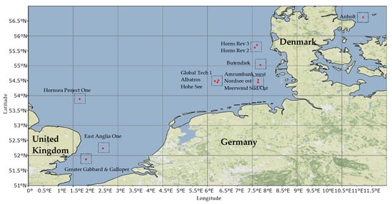
Figure 1.
Positions of the selected OWFs in the North Sea and Kattegat. The Horns Rev cluster refers to the wind farms Horns Rev 2 and 3; the Global Tech cluster refers to Global Tech 1, Albatros, and Hohe See; and the Nordsee cluster refers to Amrumbank West, Nordsee Ost, and Meerwind Süd/Ost.
Table 2.
Number of available SAR scenes before and after commissioning of each OWF and cluster.
2.3. Methods
To process the SAR scenes, four steps are applied, summarized in a flowchart (Figure 2) and explained in the following sections.
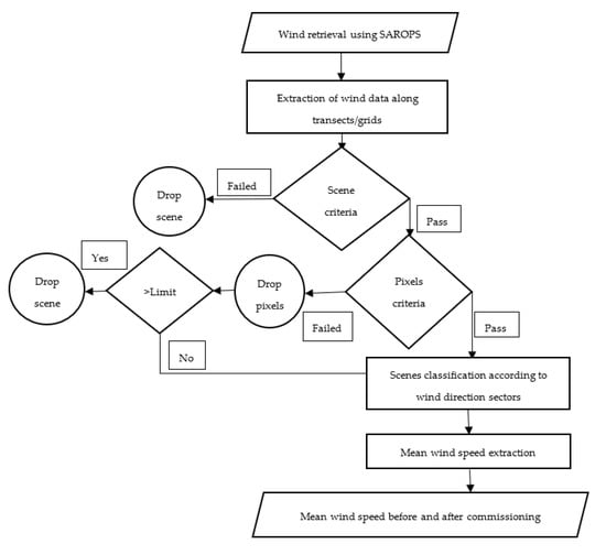
Figure 2.
Flowchart illustrating the processing steps and criteria set for the analysis of the mean wind speed from the selected SAR scenes for both investigated periods (before and after commissioning) for each site.
2.3.1. Wind Speed Retrieval from SAR
The SAR observables are related to the local near-surface wind speed through a GMF [35,36,37]. Here, we use CMOD5.N [35] to retrieve the equivalent neutral wind speed at 10 m from the radar backscatter, the radar incident angle, and the wind direction relative to the antenna look direction. Equation (1) shows the general empirical relationship between these parameters:
where is the normalized radar cross section (NRCS), is the 10 m equivalent neutral wind speed is the angle between the wind direction and the azimuth look angle of the SAR (both measured from the north), and is the radar incidence angle. The other coefficients shape the terms , and is a constant with a value of 1.6 [35].
Wind retrieval processing from SAR images requires inversion of the GMF to calculate the wind speed. Auxiliary information of wind direction from other sources, e.g., a numerical weather prediction model, is necessary to address ambiguities. In recent decades, with the advent of satellite remote sensing, the validation of GMFs and SAR wind retrieval has improved.
The SAR operational products system (SAROPS) is a set of software and protocols used to convert SAR scenes into wind maps using any GMF [38]. SAROPS has been developed at the Applied Physics Laboratory at Johns Hopkins University and the National Ocean and Atmospheric Agency in the United States. To retrieve wind speeds from SAR observations, input wind directions are taken from the Climate Forecast System Reanalysis until 2010 and from the Global Forecasting System from 2011 onward at 0.5° × 0.5° or 0.25° × 0.25° latitude–longitude sampling to initiate wind speed retrievals. SAROPS comes with masks to eliminate areas covered by land or sea ice. The original SAR data are averaged to 500-m grid cells prior to wind retrieval processing.
2.3.2. Extraction of Wind Speeds
To investigate the impact of OWF commissioning on the wind speeds, we extract wind speeds and directions along transect lines on four sides of each OWF. These lines are located 1–2 km away from the edges of OWFs and clusters except for the west side of Hornsea Project One. Due to construction of phase two on the west of the OWF, we place the transect lines about 5 km away from the west side to avoid crossing the construction sites. Transect lines enclose the entire area of the OWFs and clusters. Furthermore, extra marginal areas around OWFs and clusters are also enclosed by transect lines to study the airflow variation in these areas. The distances between the transect lines depend mainly on the dimensions of the OWFs and clusters and range from 18 to 55 km. Each transect line consists of 15 uniformly distributed points, called transect points, which are labeled from P1 to P15 and ascend from south to north for west and east transect lines and from west to east for north and south transect lines. Each transect point represents the average of a rectangular bin of the following dimensions: 3.2 km perpendicular to the transect direction and 2.5 km parallel to the transect direction. Figure 3 depicts the selected OWFs and clusters in this study and gives more details about transect lines, transect points, wind turbine coordinates, and wind roses at the transect point P7 on the west of the OWFs and clusters. The prevailing wind direction is from west or southwest for all sites, sometimes coming from the easterly wind sectors, and rarely from the north at eight sites. Accordingly, the northern wind sectors are not considered in the study due to a low number of SAR scenes.
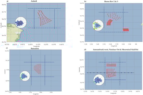
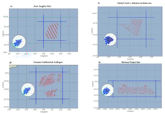
Figure 3.
Selected OWFs and clusters: (a) Anholt, (b) Horns Rev 2 and 3, (c) Butendiek, (d) Amrumbank West, Nordesee Ost, and Meerwind Süd/Ost, (e) East Anglia One, (f) Global Tech 1, Albatros, and Hohe See, (g) Greater Gabbard and Galloper, and (h) Hornsea Project One. The blue lines are the transect lines around the OWFs and clusters, and the green points are the transect points and distributed uniformly along the transect lines. The red points are the positions of wind turbines, and the wind roses represent the wind direction taken from all available scenes at the transect point P7 at the west transect line.
Before calculating the mean wind speeds of rectangular bins of transect lines, our set of SAR scenes in Table 1 is filtered according to the following criteria:
- The wind speed is between the cut-in (4 m/s) and cut-out (25 m/s) wind speed of the wind turbines to ensure that the turbines are in operation.
- The wind direction is from the easterly (45–135°), westerly (225–315°), and southerly (135–225°) sectors. Wide sector angles are considered to increase the number of samples for each case.
- The SAR wind maps fully cover the transect lines.
- Manual inspection is performed of the anomalous wind maps that have high or low wind speed to be sure that these scenes do not have any evidence of non-wind phenomena, such as processing artifacts and rain contamination.
To eliminate the effects of hard targets in the SAR images (e.g., reflection from ships) or other phenomena, such as oil spills in seas, we set a threshold value of 0.001–2 dB for SAR-normalized NRCS to skip the anomalous pixels from the analysis. To make sure that a significant number of pixels represent the wind speeds at each transect point, the ratio of dropped pixels to the original number of pixels inside a rectangular bin should not exceed 0.5. Otherwise, the scene is left out of the calculation.
The available number of SAR scenes corresponding to each wind sector are listed in Table 3. The ratios between the number of scenes after commissioning and the number of scenes before commissioning are given as well. These ratios were low for some OWFs because they were in service for a few years only. Therefore, we have fewer acquisitions after their commissioning compared with the period before the commissioning. About 8700 scenes in total passed our criteria.
Table 3.
Westerly, easterly, and southerly classified SAR wind maps for the periods before and after commissioning of the selected OWFs and clusters.
2.3.3. Mean Wind Speed Calculation
We calculate the mean wind speed for each transect point before and after commissioning of the OWFs and clusters for the classified SAR scenes based on wind sector values in Section 2.3.2. As a result, each transect point has two mean speed values, one for before and one for after the commissioning of the OWFs and clusters.
2.3.4. Velocity Deficit Calculation
The periods before and after wind farm commissioning might be subjected to differences in the overall mean wind climate. To consider such differences, we normalize the SAR wind speeds extracted downstream of the OWFs and clusters with SAR wind speeds extracted upstream of the OWFs, and clusters during the same period by calculating the percentile of the velocity deficit (). is formulated mathematically as:
where is the mean wind speed (m/s) at the transect point on the upstream side and is the mean wind speed (m/s) at the corresponding transect point on the downstream side. A positive indicates an area with a reduced wind speed, e.g., caused by wake or HCWSG effects on the downstream side of the OWF.
2.3.5. Horizontal Coastal Wind Speed Gradient Calculation
Most of the selected OWFs in this study are located within the coastal zones and are less than 50 km from the coastline. Subsequently, a number of issues arise due to (Ι) the surface discontinuity at the coastline, (ΙΙ) the influence of onshore topography, and (ΙΙΙ) thermal gradients [20]. Wind speed variations caused by these phenomena may lead to overestimation or underestimation of the magnitude of wind wakes. To differentiate between the effects of HCWSGs and the effect of wind farm wakes, we use the SAR wind maps to compute the average normalized velocity deficit before OWFs commissioning. We then subtract this gradient from the velocity deficits after the commissioning of OWFs as follows:
where is the normalized velocity deficit at the transect point due to the commissioning of the OWF and without gradients effects, is the velocity deficit after commissioning, and is the velocity deficit before commissioning of the OWF at the same transect point. is computed for all transect points based on Equation (2). The last term indicates the effects of HCWSGs on wind speed variations. HCWSGs can lead to an increase or decrease in the wind speed. Whereas offshore winds blow from the land toward the sea and onshore winds blow from the sea toward the land, both wind variations relate to the onshore distance.
2.3.6. Wind Power Variation along the Centerline of the Nordsee Cluster
For the Nordsee cluster, we calculate the wind power density along the centerline extending about 60 km to the west and east side of the cluster (see Figure 3d). The mean wind power density is computed based on the following equation for all points along the line:
where is the density of air (1.255 kg/m3) and is the mean of the cubed velocity series (m/s) at the blue points along the centerline in Figure 3d. The calculation has been performed only on the scenes from the period after OWF commissioning and for westerly and easterly wind sectors only.
3. Results
In this section, we present sector-wise wind speeds, velocity deficits upstream vs. downstream and before vs. after commissioning of the eight sites (three clusters and five OWFs), and the variation in HCWSGs before the commissioning of OWFs. We show that HCWSGs near the coast can have a significant impact on the wind speeds for the near-coastal OWFs, and we correct for such gradients. The Nordsee cluster is taken as an example to show the wind power variation upstream and downstream of a cluster. Finally, we demonstrate how the size of OWFs in terms of the capacity is correlated with the maximum velocity deficits downstream of the OWFs.
3.1. Mean Wind Speed and Velocity Deficit: Westerly Winds
Figure 4 shows variations in the mean wind speed when the wind blows from westerly directions. Three clusters (Global Tech, Nordsee, and Horns Rev) and the Butendiek OWF are then exposed to winds from the open ocean, whereas the other four (Hornsea Project One, East Anglia One, Greater Gabbard and Galloper, and Anholt) are exposed to winds coming from the land. The blue curves represent the ‘background’ wind conditions before the OWFs were commissioned. We find a reduction in the wind speeds as the wind approaches the coastlines (Figure 4b–d) and an increase in the wind speeds as the winds blow from the land to sea (Figure 4a,e–h). Once the OWFs are operating (green curves), we can detect a clear reduction in the wind speeds on the downstream side of most of the sites, except for Anholt and Greater Gabbard and Galloper. This reduction is on the order of 0.5 m/s for the transect points directly downstream of the OWFs, and we anticipate that it is caused by the wind turbines.
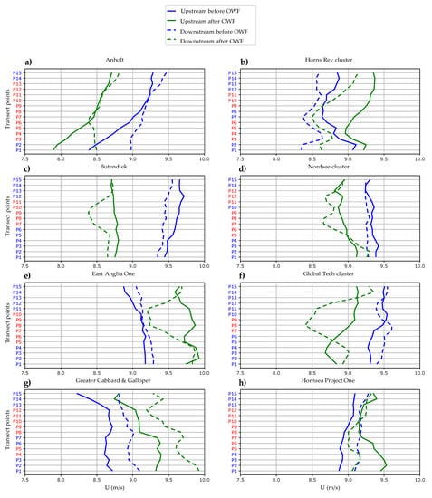
Figure 4.
Mean wind speed ( for westerly winds over the OWFs and clusters. The blue and green curves refer to periods before and after OWF commissioning, respectively. Solid lines represent the upstream side and the dashed lines the downstream side of the OWFs. The red-labeled transect points are those located directly upstream/downstream of the wind turbines (see also Figure 3). (a) Anholt; (b) Horns Rev cluster; (c) Butendiek; (d) Nordsee cluster; (e) East Anglia One; (f) Global Tech cluster; (g) Greater Gabbard & Galloper; (h) Hornsea Project One.
Figure 4 also shows that the mean wind conditions before and after the OWF commissioning can be different. If the mean wind climate was consistent for the two periods, the solid blue and green curves would overlap, but this is not the case. The plots show differences of up to ±1 m/s.
For many OWFs and clusters, it is easy to identify the potential areas of wind wakes based on the differences between upstream and downstream speed values. Nevertheless, as the OWFs are close to the coast at Anholt and the Greater Gabbard and Galloper site (Figure 4a,g), the areas of wind wakes are not obvious. Apparently, the shore distance controls, to a certain extent, the appearance of wind wakes.
Figure 5 shows the magnitude of velocity deficits for each site (i.e., the difference between of the OWFs and clusters before and after the commissioning). The blue curves illustrate the conditions before the OWFs were commissioned and should, ideally, remain close to 0% but due to the HCWSGs, they deviate from this value. The green curves show velocity deficits after the OWFs were commissioned. Positive values indicate a reduction in the wind speeds, and we observe this for all the OWFs except at Greater Gabbard and Galloper. When the positive or negative values of the background HCWSGs are subtracted from the velocity deficits, a consistent pattern emerges with velocity deficits directly downstream of every OWF. This deficit ranges from 1% at Greater Gabbard and Galloper to 8% for Global Tech 1. Toward the end points of the transect lines, the magnitudes of velocity deficits are smaller or even negative, which means that the wind speeds increased at the edges of most OWFs and clusters (Figure 5a–d,f,g).
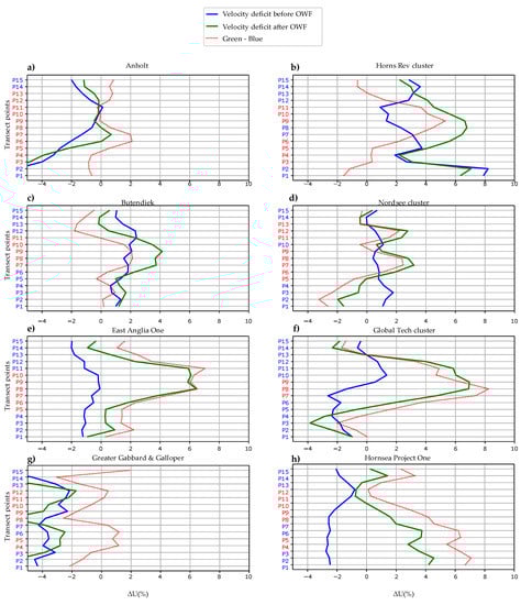
Figure 5.
Velocity deficit ( for westerly winds over the OWFs and clusters. The blue and green curves refer to periods before and after OWF commissioning, respectively. The red dotted line shows the s once a correction for HCWSGs has been applied (i.e., subtraction of the blue curve from the green). (a) Anholt; (b) Horns Rev cluster; (c) Butendiek; (d) Nordsee cluster; (e) East Anglia One; (f) Global Tech cluster; (g) Greater Gabbard & Galloper; (h) Hornsea Project One.
3.2. Mean Wind Speed and Velocity Deficit: Easterly Winds
Figure 6 shows the wind speed variation for easterly wind directions. Now, the Horns Rev and Nordsee cluster and Butendiek are exposed to winds coming from the land whereas Anholt, Hornsea Project One, East Anglia One, the Global Tech cluster, and Greater Gabbard and Galloper are exposed to winds from the open ocean. We see a gradient in the background wind speed before OWF commissioning (blue curves) for all the OWFs, but this gradient is most pronounced for Horns Rev, Butendiek, the Nordesee cluster, and Hornsea Project One (Figure 6b–d,h). As for the westerly wind sectors, we find that the undisturbed upstream wind speed is different for the periods before and after OWF commissioning. The largest differences, exceeding 1 m/s, are seen for the newer OWFs, where a relatively low number of satellite samples exist after the commissioning (see Table 3 and Figure 6e–g).
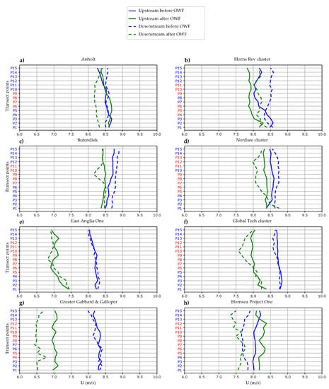
Figure 6.
Mean wind speed ( for easterly winds over the OWFs and clusters. See Figure 4 for the line definitions. (a) Anholt; (b) Horns Rev cluster; (c) Butendiek; (d) Nordsee cluster; (e) East Anglia One; (f) Global Tech cluster; (g) Greater Gabbard & Galloper; (h) Hornsea Project One.
For the easterly wind sectors, we see reduced wind speeds downstream of Anholt, Butendiek, the Nordsee cluster and Greater Gabbard and Galloper, and Hornsea Project One (Figure 6a,c,d,g,h), which we assume to be caused by wind farm wake effects. The effect is less pronounced than for the westerly wind sectors. Once we calculate the velocity deficits, i.e., the difference between upstream and downstream wind speeds and account for the effect of HCWSGs, a clear pattern emerges, showing a velocity deficit for all OWFs and clusters, as illustrated in Figure 7. The deficit ranges from 2% at East Anglia One to almost 10% at Hornsea Project One, but it is also negative for some points along the transect lines (Figure 7b,d–f).
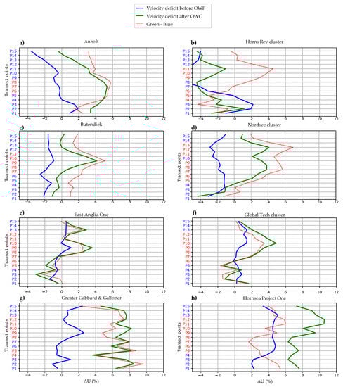
Figure 7.
Velocity deficit ( for easterly winds over the OWFs and clusters. See Figure 5 for the definitions of lines. (a) Anholt; (b) Horns Rev cluster; (c) Butendiek; (d) Nordsee cluster; (e) East Anglia One; (f) Global Tech cluster; (g) Greater Gabbard & Galloper; (h) Hornsea Project One.
3.3. Mean Wind Speed and Velocity Deficit: Southerly Winds
When winds are coming from southerly directions, all the eight sites are exposed to winds from the land but the fetch is variable. The blue curves in Figure 8 indicate that the HCWSGs before sites’ commissioning dates are always smaller than 0.5 m/s, whereas larger gradients are found for the westerly and easterly wind sectors for some of the OWFs. Again, we find significant changes in the wind speeds for the periods before and after commissioning, especially at Horns Rev, Butendiek, and Greater Gabbard and Galloper (Figure 8b,c,g). The green curves show that the wind speed is lower after OWF commissioning for all the OWFs except the Horns Rev cluster and Hornsea Project One (Figure 8b,h).
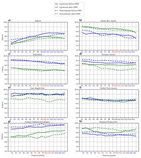
Figure 8.
Mean wind speed ( for southerly winds over the OWFs and clusters. See Figure 4 for the line definitions. Note that the figure axes are different than for the corresponding plots for westerly and easterly winds as we have chosen to match the layout of transects in Figure 3. (a) Anholt; (b) Horns Rev cluster; (c) Butendiek; (d) Nordsee cluster; (e) East Anglia One; (f) Global Tech cluster; (g) Greater Gabbard & Galloper; (h) Hornsea Project One.
The velocity deficit is most pronounced directly downstream of the OWFs and clusters. Because of the large sector angles (90) considered in the SAR wind maps classification, velocity deficits are detected for the transect points located at an angle from the center of the OWFs. So, evidence of wake effects is found beyond the actual dimension of the OWFs and clusters.
Figure 9 shows velocity deficits for the southerly wind sector. After correcting for HCWSGs, we find a deficit downstream of the four OWFs (East Anglia One, Greater Gabbard, Butendiek, and Amrumbank West). The other four OWFs show fluctuating curves, changing between positive and negative velocity deficits.
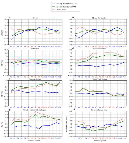
Figure 9.
Velocity deficit ( for southerly winds over the OWFs and clusters. See Figure 5 for the definitions of lines. Note that the figure axes are different than for the corresponding plots for westerly and easterly winds as we have chosen to match the layout of transects in Figure 3. (a) Anholt; (b) Horns Rev cluster; (c) Butendiek; (d) Nordsee cluster; (e) East Anglia One; (f) Global Tech cluster; (g) Greater Gabbard & Galloper; (h) Hornsea Project One.
3.4. Horizontal Coastal Wind Speed Gradient Variation before OWFs
HCWSGs can lead to increased or decreased wind speeds along the dimension of OWFs. The positive and negative values refer to decreased or increased wind speed, respectively. The westerly and easterly winds are classified into onshore and offshore winds in Figure 10b,c, based on the wind direction with respect to land and ocean. The southerly winds are offshore winds with variable fetch. As shown in Figure 10, the offshore winds increased for all sites except for Hornsea Project One (it is the OWF furthest from the coast in this study). However, the onshore winds decreased in the Horns Rev cluster, Butendiek, and Hornsea Project One and increased in Anholt, East Anglia One, and the Global Tech cluster and increased slightly in the Nordsee cluster.
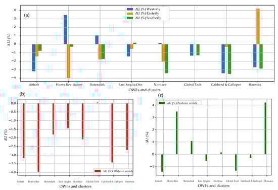
Figure 10.
Velocity deficit ( variation for (a) all wind sectors at the investigated sites, (b) offshore, and (c) onshore winds. Only westerly and easterly wind sectors are considered to be offshore and onshore winds.
3.5. The Nordsee Cluster
To visualize the spatial variability of velocity deficits, two velocity deficit maps are shown in Figure 11 for the Nordsee cluster, with westerly and easterly winds. As shown in Figure 5d and Figure 7d, at the transect point P10, there was a drop in the velocity deficit for both westerly and easterly winds. The upstream mean wind speed values for both westerly and easterly wind cases are taken as the average of velocity inside the drawn rectangles in front of the cluster. For westerly winds, the highest values of velocity deficits are directly downstream of the Amrumbank West and Nordsee Ost OWFs. Between the two OWFs is the pre-construction site for the future Kaskasi OWF, which is currently turbine-free. Therefore, we see a lower velocity deficit near the transect point P10 compared with adjacent transect points. Similarly for the easterly wind sector, the highest deficits are found directly behind the two existing OWFs. This example illustrates that mean velocity deficits exceeding 3% can be detected up to 21 km downstream of large OWFs. Although the number of SAR scenes used to generate Figure 11b is two times more than in Figure 11a, the velocity deficit area (with > 3%) is bigger for easterly than for westerly winds. Subsequently, the wind power variation is larger for the easterly rather than the westerly wind sector, as shown in Section 3.6. The mean wind speed of easterly winds was about 0.8 m/s slower than for westerly wind directions (see Figure 4d and Figure 6d).
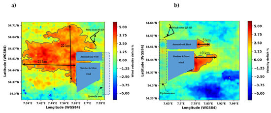
Figure 11.
Map of the velocity deficit ( around the Nordsee cluster calculated from the SAR wind maps in Table 3 for (a) easterly winds and (b) westerly winds at 10 m m.s.l. The contour lines show the area where the exceeds 3%. The dashed rectangle shows the area used for calculating the upstream wind velocity.
3.6. Wind Power Variation along the Centerline of the Nordsee Cluster
Figure 12 reveals the variations in wind speeds and wind power densities along the centerline going through the Nordsee cluster. As the winds approach the cluster, there is a steep reduction in power density and the maximum loss is at points close to the cluster (within 5 km from the outer edge of the cluster). As the winds pass the OWF, the energy density reduces and remains so for 10–20 km downstream. Afterward, the mean wind power density ( increases. The reduction in on the upstream and downstream sides of the OWF may refer to the blockage effects of the cluster and the wind wakes of turbines, respectively [39].
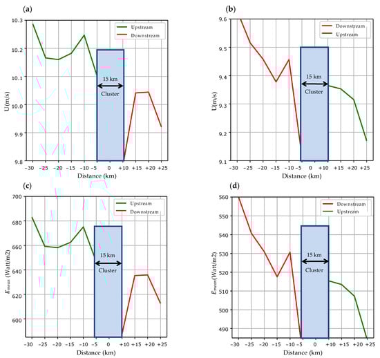
Figure 12.
(a,b) Mean wind speed ( variation along the centerline of the Nordsee cluster for westerly and easterly winds at 10 m above m.s.l., respectively. (c,d) Mean wind power density ( variation (watt/m2) along the centerline of the Nordsee cluster for westerly and easterly winds, respectively. The black solid rectangle refers to the position of the cluster, and the + and − signs refer to the right and left of the cluster.
3.7. Impact of the OWF and Cluster Capacity
To investigate the relation between the velocity deficit at transect lines and the capacity of the OWFs and clusters, we show the maximum velocity deficits for each wind sector in Table 4. The velocity deficit depends mainly on the magnitude of wind speeds and not on the wind direction. Therefore, we average the maximum velocity deficits for all directional sectors.
Table 4.
Maximum velocity deficit ( detected within the first 5 km downstream of the OWFs and clusters.
Figure 13 reveals how the OWF and the cluster capacities are proportional with the average maximum velocity deficit. As the capacity increases, the velocity deficit increases as well. The best fit line equation for the observations is shown with R2 = 0.67.
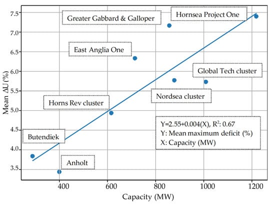
Figure 13.
The average maximum velocity deficit for westerly, easterly, and southerly winds; average maximum ΔU in Table 4 vs. the capacity of OWFs and clusters.
4. Discussion
In this study, we have exploited the abundance of SAR data, which is free and open-access for researchers and the industry, to analyze the impact of eight installed OWFs and clusters on the wind speed variation. We have used transects and gridded maps to extract wind speeds from an area of interest around each OWF and cluster. Previous studies have used the transect principle to extract the wind speed and directions in order to quantify wind wakes downstream of OWFs and clusters [5,25,26,40].
4.1. Wind Conditions before OWFs Are Commissioned
Before OWFs and clusters are commissioned, we should in principle see that wind conditions are similar for the upstream and downstream sides of the yet-to-be-commissioned OWFs. However, the wind speeds extracted upstream and downstream can be different because of HCWSGs. HCWSGs can lead to an increase/decrease in the upstream and downstream wind speed on the order of 4% for offshore and onshore winds, which may be larger than the wake-induced velocity deficit. The computed natural wind speed gradients in Figure 10 show the large spatial wind variation within the coastal area. This fits well with Hasager’s outcome in [17]. Therefore, we have chosen to correct for the background wind speed gradient before computing turbine-induced velocity deficits.
4.2. Wind Conditions after OWFs Are Commissioned
Based on the transect analysis, we can detect a velocity deficit downstream of the OWFs and clusters in 22 out of 24 situations investigated (eight sites and three directional sectors). A positive velocity deficit indicates that the wind speed is reduced with respect to the wind speed on the upstream side of each OWF and cluster. The magnitude of the velocity deficits varies a lot (1 to 10%) for the different sites and wind directions. It is important to keep in mind that the velocity deficits are obtained 10 m above the sea surface. Presumably, the deficits are much larger at the heights of the turbine hub and rotor plane. Because we have analyzed 90° wide directional sectors, the maximum velocity deficit is sometimes displaced and does not necessarily coincide with the area immediately to the east, west, or north of the wind turbines. Two sets of results do not fit well with our expectations: For westerly winds around Greater Gabbard and Galloper (Figure 5g) and for southerly winds around the Hornsea Project One (Figure 9h), we cannot detect any velocity deficit along the transects located downstream of the wind turbines. Results for the Anholt site presented by Ahsbahs et al. [5] fit well with our results. However, in this study, we consider longer periods and we use a wider range of wind directions compared to previous works.
4.3. Temporal Wind Speed Variations
Wind speeds extracted on the upstream side of each wind farm should, in principle, show similar wind speed values before and after OWF commissioning. However, in most investigated cases here, we find differences larger than 0.5 m/s. It is possible that the actual wind speed is different for the periods analyzed here (i.e., before and after OWF commissioning). The wind climate in the northern European seas normally shows annual variabilities on the order of ±5% [41]. Another possible reason for the differences could be the unbalanced number of SAR scenes before and after commissioning of the OWFs and clusters (as shown in Table 3). Lastly, Badger et al. [11] showed that early SAR observations from Envisat have calibration issues, which could impact the calculated velocity deficits for the period 2002–2012.
In addition to the annual wind speed variation, there is seasonal wind speed variability in the northern European seas [41]. This seasonality may impact our results as follows: Wind speed retrieval based on the GMF CMOD5.N assumes neutral atmospheric conditions, but Pena et al. [42] showed that the area is on average prone to slightly unstable conditions, which may lead to an underestimation of the retrieved wind speeds. Unstable conditions are mostly seen during autumn and winter, when the wind climate is governed by atmospheric fronts and moderate to high wind speeds. Stable conditions are more pronounced in the springtime and with low wind speeds, and they can lead to overestimation of instantaneous wind speed retrievals. As shown in Figure 3, the prevailing and dominant wind directions are from the westerly and south-westerly sectors for all eight sites, so our dataset could be biased toward unstable atmospheric conditions. However, since we are dealing with relative differences in the wind speed (upstream vs. downstream and before vs. after commissioning), this should not have any major impact on our findings.
Atmospheric stability can also impact the magnitude and spatial extent on wind turbine wakes. Typically, wakes persist for longer periods during stable conditions as the degree of atmospheric mixing is low [43,44]. Good examples of where this is seen in SAR imagery are available in the literature (e.g., [31,45]). A bias in the satellite sampling between seasons (or diurnally) could have a direct impact on the average of velocity deficits we have estimated. Further investigation is necessary to fully determine the effects of atmospheric stability.
4.4. Effects of the Wind Farm Size and Layout
For the Nordsee cluster, we have demonstrated how gridded maps can help visualize and understand the wind farm effects on the mean wind climate in the area surrounding the OWFs (Figure 11). We can use such maps to locate the maximum velocity deficit on the downstream side of the cluster. The Nordsee cluster is particularly interesting because it includes a preconstruction site for the future Kaskasi OWF, which is currently turbine-free. In the future, we will be able to see how the closing of this gap with new turbines will impact the wind climate in the area. This example illustrates the reason for variation in velocity deficit along the transect line. A similar turbine-free area is Greater Gabbard and Galloper (see Figure 3g); this causes a precipitous decline in the velocity deficit at transect points in front of the turbine-free area (see Figure 5g and Figure 7g).
Based on wind speeds and velocity deficits extracted from our set of SAR wind maps, we have established a relationship between the total capacity of OWFs or clusters and the average maximum velocity deficits of westerly, easterly, and southerly winds. The linear relation may not be the best suited to describe the maximum velocity deficit vs. capacity given that the wind power density is proportional to the wind speed cubed. However, it gives the clear impression that larger OWFs generate the most pronounced velocity deficits in the surrounding areas. Other characteristics of OWFs should be considered as well, in order to improve the model. For example, the turbine size, the density of wind turbines, and their layout with respect to the wind direction can be expected to influence the wind farm wakes we can detect with SAR. Hornsea Project One is the biggest OWF in the study, and its layout extends more horizontally than vertically (Figure 3h). The velocity deficits for westerly and easterly winds are higher than for southerly winds. Subsequently, Figure 9h does not show wind wakes in most of the transect points.
Because the wind power density is proportional to the wind speed cubed, velocity deficits similar to the ones detected here have a direct impact on the wind power density in an area. We have quantified this impact for the Nordsee cluster (Figure 12) along the centerline of the cluster (Figure 3d). Here, we detect velocity deficits along the centerline up to 2% downstream of the wind turbines and this is equivalent to energy losses up to 6.5%. We also see a variation in the wind power density on the upstream side of the turbines (Figure 12a). This might be caused by blockage effects of the cluster itself [39].
4.5. Future Perspectives
In addition to the wind-related effects discussed above, we would like to stress that additional phenomena can affect the SAR wind retrieval accuracy and thus the results presented here. High backscattering originating from man-made objects at sea (e.g., wind turbines, ships, and oil refineries) are inevitably in the areas surrounding OWFs and clusters. We have filtered out the most extreme values, but more advanced methods exist for removing these bright targets. OWFs are typically constructed where the water depth is shallow. Hence, the underwater bathymetry can cause a signal due to modulation of the capillary and short-gravity waves that a C-band SAR system is sensitive to. Finally, ocean waves and their effects are still ambiguous, especially since wave patterns can be complex in the vicinity of wind turbine towers.
In the future, we advocate the following improvements in our approach:
- Replace the threshold of the NRCS to remove anomalous SAR backscatter values caused by man-made objects with other sophisticated object detectors, such as a constant false alarm ratio.
- Account for the atmospheric stability conditions when SAR scenes are classified.
- Validate wind speeds and velocity deficits retrieved from SAR at different sites using, e.g., wind LiDAR, airborne observations, or turbine SCADA data.
- Extrapolate our results up to the wind turbine hub height to make the findings more suitable for offshore wind energy applications.
5. Conclusions
This study has demonstrated how wind speeds retrieved from SAR can be used to quantify the impact of large OWFs on the wind climate in their surroundings. Most wind power installations today are in coastal areas. Hence, they have a significant impact on marine coastal environments. At the same time, strong HCWSGs are observed in coastal areas, which makes it challenging to estimate the spatial and temporal wind speed changes induced by the OWF. Thanks to the enormous archive of satellite SAR scenes available from Envisat and Sentinel-1, we can map the wind conditions before and after a given OWF is commissioned. For the first time, this has been used to perform systematic OWF wake analyses over many sites. We find that a significant velocity deficit, along with an associated potential power loss, occurs downstream of large OWFs. The velocity deficits are proportional to the total OWF capacity. The use of SAR data for mapping of OWF wake effects could be beneficial in the context of wind farm planning. For example, SAR wind maps could indicate the wind speed recovery distance and help to determine the feasibility of new wind farm projects in the vicinity of existing projects.
Author Contributions
A.O. decided on the direction of the study with the help from M.B., implemented the complete workflow in Python, performed the literature works, and followed the author’s feedback and suggestions. M.B. supervised the project works and proposed many research questions covered in this study. All authors have read and agreed to the published version of the manuscript.
Funding
This work has been conducted under the Innovation Training Network Marie Skłodowska-Curie Action Train2Wind. Train2Wind has received funding from the European Union Horizon 2020 (Grant agreement ID: 861291).
Institutional Review Board Statement
Not applicable.
Informed Consent Statement
Not applicable.
Data Availability Statement
Further information about the Sentinel-1 mission is available at https://sentinel.esa.int/web/sentinel/missions/sentinel-1 (last access: 15 December 2020 and information about the Envisat mission is available at https://earth.esa.int/eogateway/missions/envisat/description (last access: 31 January 2022). The archive of SAR wind maps from the Technical University of Denmark (DTU) is available at https://science.globalwindatlas.info/#/map/satwinds (last access: 31 January 2022). Raw Sentinel-1 and Envisat data are available at the Copernicus Open Access Hub of ESA via https://scihub.copernicus.eu/dhus/#/home (last access: 31 January 2022).
Acknowledgments
We would like to acknowledge the funding from the European Union Horizon 2020 to the Train2Wind network. We thank the Johns Hopkins University, Applied Physics Laboratory and the National Oceanic and Atmospheric Administration in the United States for the use of the SAROPS system, and ESA for providing public access to data from Sentinel 1A/B and Envisat. Personal thanks to Dalibor Cavar and Ebba Dellwik for their constructive comments to the manuscript and to Ioanna Karagali and Oscar Garcia for their support in using the High Processing Cluster system at DTU (HPC/DTU). A special thanks goes to five anonymous reviewers of the manuscript.
Conflicts of Interest
The authors declare no conflict of interest.
Abbreviation
The following abbreviations are used in this manuscript:
| SAR | Synthetic Aperture Radar |
| OWF | Offshore Wind Farm |
| NRCS | Normalized Radar Cross Section |
| RMSE | Root Mean Square Error |
| CFD | Computational Dynamics Models |
| LiDAR | Light Detection and Ranging |
| GMF | Geophysical Model Function |
| VV | Vertical Polarized |
| SAROPS | SAR Operational Products System |
| CMOD5.N | C-Band Model 5.N |
References
- Wilson, J.C.; Elliott, M.; Cutts, N.D.; Mander, L.; Mendão, V. Coastal and Offshore Wind Energy Generation: Is it environmentally benign. Energies 2010, 3, 1383–1422. [Google Scholar] [CrossRef]
- Sesto, E.; Lipman, N.H. Wind Energy in Europe. Wind Europe, Brussels Belgium. 2020. Available online: https://gwec.net/global-offshore-wind-report-2021/ (accessed on 8 March 2022).
- Rana, F.M.; Adamo, M.; Lucas, R.; Blonda, P. Sea surface wind retrieval in coastal areas by means of Sentinel-1 and numerical weather prediction model data. Remote Sens. Environ. 2019, 225, 379–391. [Google Scholar] [CrossRef]
- Hasager, C.B.; Hahmann, A.N.; Ahsbahs, T.; Karagali, I.; Sile, T.; Badger, M.; Mann, J. Europe’s offshore winds assessed with synthetic aperture radar, ASCAT and WRF. Wind Energy Sci. 2020, 5, 375–390. [Google Scholar] [CrossRef] [Green Version]
- Ahsbahs, T.; Badger, M.; Volker, P.; Hansen, K.S.; Hasager, C.B. Applications of satellite winds for the offshore wind farm site Anholt. Wind Energy Sci. 2018, 3, 573–588. [Google Scholar] [CrossRef] [Green Version]
- Allan, T.D. Remote Sensing of the European Seas: A Historical Outlook; Springer: Dordrecht, The Netherlands, 2008; ISBN 9781402067716. [Google Scholar]
- Dagestad, K.-F.; Horstmann, J.; Mouche, A.; Perrie, W.; Shen, H.; Zhang, B.; Li, X.; Monaldo, F.; Pichel, W.; Lehner, S.; et al. Wind Retrieval from Synthetic Aperture Radar—An Overview. In Proceedings of the 4th SAR Oceanography Workshop (SEASAR 2012), Tromsø, Norway, 18–22 June 2012; pp. 18–22. [Google Scholar]
- Wang, H.; Yang, J.; Mouche, A.; Shao, W.; Zhu, J.; Ren, L.; Xie, C. GF-3 SAR oceanwind retrieval: The first view and preliminary assessment. Remote Sens. 2017, 9, 694. [Google Scholar] [CrossRef] [Green Version]
- Hasager, C.B.; Peña, A.; Christiansen, M.B.; Astrup, P.; Nielsen, M.; Monaldo, F.; Thompson, D.; Nielsen, P. Remote sensing observation used in offshore wind energy. IEEE J. Sel. Top. Appl. Earth Obs. Remote Sens. 2008, 1, 67–79. [Google Scholar] [CrossRef] [Green Version]
- Valenzuela, G.R. Theories for the interaction of electromagnetic and oceanic waves—A review. Bound.-Layer Meteorol. 1978, 13, 61–85. [Google Scholar] [CrossRef]
- Badger, M.; Ahsbahs, T.; Maule, P.; Karagali, I. Inter-calibration of SAR data series for offshore wind resource assessment. Remote Sens. Environ. 2019, 232, 111316. [Google Scholar] [CrossRef] [Green Version]
- Jagdish; Kumar, S.V.V.A.; Chakraborty, A.; Kumar, R. Validation of wind speed retrieval from RISAT-1 SAR images of the North Indian Ocean. Remote Sens. Lett. 2018, 9, 421–428. [Google Scholar] [CrossRef]
- Wang, H.; Shi, C.; Zhu, J. Assessment of Sentinel-1A/B SAR Derived Ocean Wind Speeds against Scatterometer in the Presence of Ocean Swells. E3S Web Conf. 2021, 299, 01001. [Google Scholar] [CrossRef]
- Ahsbahs, T.; Badger, M.; Karagali, I.; Larsén, X.G. Validation of sentinel-1A SAR coastal wind speeds against scanning LiDAR. Remote Sens. 2017, 9, 552. [Google Scholar] [CrossRef] [Green Version]
- J¢rgensen, B.H.; Furevik, B.; Hasager, C.B.; Astrup, P.; Rathmann, O.; Barthelmie, R.J.; Pryor, S.C. Off-shore wind fields obtained from mesoscale modeling and satellite SAR images. In Proceedings of the EWEA Offshore Wind Energy Special Topic Conference, Brussels, Belgium, 12 October 2001; pp. 2–5. [Google Scholar]
- Takeyama, Y.; Ohsawa, T.; Kozai, K.; Hasager, C.B.; Badger, M. Comparison of geophysical model functions for SAR wind speed retrieval in Japanese coastal waters. Remote Sens. 2013, 5, 1956–1973. [Google Scholar] [CrossRef] [Green Version]
- Hasager, C.B. Offshore winds mapped from satellite remote sensing. Wiley Interdiscip. Rev. Energy Environ. 2014, 3, 594–603. [Google Scholar] [CrossRef] [Green Version]
- Cameron, I.; Lumsdon, P.; Walker, N.; Woodhouse, I. Synthetic Aperture Radar for Offshore Wind Resource Assessment and Wind Farm Development in the UK. In Proceedings of theSEASAR 2006: Advances in SAR Oceanography from Envisat and ERS Missions, Frascati, Italy, 23–26 January 2006; Volume 613, pp. 1–6. [Google Scholar]
- Doubrawa, P.; Barthelmie, R.J.; Pryor, S.C.; Hasager, C.B.; Badger, M.; Karagali, I. Satellite winds as a tool for offshore wind resource assessment: The Great Lakes Wind Atlas. Remote Sens. Environ. 2015, 168, 349–359. [Google Scholar] [CrossRef] [Green Version]
- Barthelmie, R.J.; Badger, J.; Pryor, S.C.; Hasager, C.B.; Christiansen, M.B.; Jørgensen, B.H. Offshore coastal wind speed gradients: Issues for the design and development of large offshore windfarms. Wind Eng. 2007, 31, 369–382. [Google Scholar] [CrossRef]
- Romeiser, R.; Ufermann, S.; Kern, S. Status report on the remote sensing of current features by spaceborne synthetic aperture radar. In Proceedings of the 2nd Workshop Coastal Marine Application SAR, Hamburg, Germany, 3 June 2004; pp. 105–123. [Google Scholar]
- Hasager, C.; Astrup, P.; Barthelmie, R.; Dellwik, E. Validation of Satellite SAR Offshore Wind Speed Maps to In-Situ Data, Microscale and Mesoscale Model Results; Forskningscenter Risoe: Roskilde, Denmark, 2002; Volume 1298, ISBN 8755029590. [Google Scholar]
- Hasager, C.B.; Nygaard, N.G.; Volker, P.J.H.; Karagali, I.; Andersen, S.J.; Badger, J. Wind farm wake: The 2016 Horns Rev photo case. Energies 2017, 10, 317. [Google Scholar] [CrossRef] [Green Version]
- Porté-agel, F. Wind-Turbine and Wind-Farm Flows: A Review. Bound.-Layer Meteorol. 2020, 174, 1–59. [Google Scholar] [CrossRef] [Green Version]
- Christiansen, M.B.; Hasager, C.B. Wake effects of large offshore wind farms identified from satellite SAR. Remote Sens. Environ. 2005, 98, 251–268. [Google Scholar] [CrossRef]
- Ahsbahs, T.; Nygaard, N.G.; Newcombe, A.; Badger, M. Wind farm wakes from SAR and doppler radar. Remote Sens. 2020, 12, 462. [Google Scholar] [CrossRef] [Green Version]
- Barthelmie, R.J.; Pryor, S.C.; Frandsen, S.T.; Hansen, K.S.; Schepers, J.G.; Rados, K.; Schlez, W.; Neubert, A.; Jensen, L.E.; Neckelmann, S. Quantifying the impact of wind turbine wakes on power output at offshore wind farms. J. Atmos. Ocean. Technol. 2010, 27, 1302–1317. [Google Scholar] [CrossRef]
- Herges, T.G.; Maniaci, D.C.; Naughton, B.T.; Mikkelsen, T.; Sjöholm, M. High resolution wind turbine wake measurements with a scanning lidar. J. Phys. Conf. Ser. 2017, 854. [Google Scholar] [CrossRef] [Green Version]
- Käsler, Y.; Rahm, S.; Simmet, R.; Kühn, M. Wake measurements of a multi-MW wind turbine with coherent long-range pulsed doppler wind lidar. J. Atmos. Ocean. Technol. 2010, 27, 1529–1532. [Google Scholar] [CrossRef] [Green Version]
- Bodini, N.; Zardi, D.; Lundquist, J.K. Three-dimensional structure of wind turbine wakes as measured by scanning lidar. Atmos. Meas. Tech. 2017, 10, 2881–2896. [Google Scholar] [CrossRef] [Green Version]
- Gao, X.; Wang, T.; Li, B.; Sun, H.; Yang, H.; Han, Z.; Wang, Y.; Zhao, F. Investigation of wind turbine performance coupling wake and topography effects based on LiDAR measurements and SCADA data. Appl. Energy 2019, 255, 113816. [Google Scholar] [CrossRef]
- Platis, A.; Siedersleben, S.K.; Bange, J.; Lampert, A.; Bärfuss, K.; Hankers, R.; Cañadillas, B.; Foreman, R.; Schulz-Stellenfleth, J.; Djath, B.; et al. First in situ evidence of wakes in the far field behind offshore wind farms. Sci. Rep. 2018, 8, 2163. [Google Scholar] [CrossRef] [PubMed]
- Goit, J.P.; Shimada, S.; Kogaki, T. Can Lidars replace meteorological masts in wind energy? Energies 2019, 12, 3680. [Google Scholar] [CrossRef] [Green Version]
- Rösner, B.; Egli, S.; Thies, B.; Beyer, T.; Callies, D.; Pauscher, L.; Bendix, J. Fog and Low Stratus Obstruction of Wind Lidar Observations in Germany A Remote Sensing-Based Data Set for Wind Energy Planning. Energies 2020, 13, 3859. [Google Scholar] [CrossRef]
- Hersbach, H.; Stoffelen, A.; De Haan, S. An improved C-band scatterometer ocean geophysical model function: CMOD5. J. Geophys. Res. Ocean. 2007, 112, 1–18. [Google Scholar] [CrossRef]
- Zhang, B.; Mouche, A.; Lu, Y.; Perrie, W.; Zhang, G.; Wang, H. A Geophysical Model Function for Wind Speed Retrieval from C-Band HH-Polarized Synthetic Aperture Radar. IEEE Geosci. Remote Sens. Lett. 2019, 16, 1521–1525. [Google Scholar] [CrossRef]
- Lu, Y.; Zhang, B.; Perrie, W.; Mouche, A.A.; Li, X.; Wang, H. A C-Band geophysical model function for determining coastal wind speed using synthetic aperture radar. IEEE J. Sel. Top. Appl. Earth Obs. Remote Sens. 2018, 11, 2417–2428. [Google Scholar] [CrossRef] [Green Version]
- Monaldo, F.; Jackson, W.G.; Li, X. A weather eye on coastal winds. Eos 2015, 96. [Google Scholar] [CrossRef]
- Schneemann, J.; Theuer, F.; Rott, A.; Dörenkämper, M.; Kühn, M. Offshore wind farm global blockage measured with scanning lidar. Wind Energy Sci. Discuss. 2020, 1–26. [Google Scholar] [CrossRef]
- Hasager, C.B.; Vincent, P.; Husson, R.; Mouche, A.; Badger, M.; Peña, A.; Volker, P.; Badger, J.; Di Bella, A.; Palomares, A.; et al. Comparing satellite SAR and wind farm wake models. J. Phys. Conf. Ser. 2015, 625, 012035. [Google Scholar] [CrossRef] [Green Version]
- Karagali, I.; Badger, M.; Hahmann, A.N.; Peña, A.; Hasager, C.B.; Sempreviva, A.M. Spatial and temporal variability of winds in the Northern European Seas. Renew. Energy 2013, 57, 200–210. [Google Scholar] [CrossRef]
- Peña, A.; Gryning, S.E.; Hasager, C.B. Measurements and modelling of the wind speed profile in the marine atmospheric boundary layer. Bound.-Layer Meteorol. 2008, 129, 479–495. [Google Scholar] [CrossRef]
- Cañadillas, B.; Foreman, R.; Barth, V.; Siedersleben, S.; Lampert, A.; Platis, A.; Djath, B.; Schulz-Stellenfleth, J.; Bange, J.; Emeis, S.; et al. Offshore wind farm wake recovery: Airborne measurements and its representation in engineering models. Wind Energy 2020, 23, 1249–1265. [Google Scholar] [CrossRef]
- Neumann, T.; Emeis, S. Long-range modifications of the wind field by offshore wind parks--Results of the project WIPAFF. Meteorol. Z. 2020, 29, 355–376. [Google Scholar]
- Djath, B.; Schulz-Stellenfleth, J.; Cañadillas, B. Impact of atmospheric stability on X-band and C-band synthetic aperture radar imagery of offshore windpark wakes. J. Renew. Sustain. Energy 2018, 10, 043301. [Google Scholar] [CrossRef] [Green Version]
Publisher’s Note: MDPI stays neutral with regard to jurisdictional claims in published maps and institutional affiliations. |
© 2022 by the authors. Licensee MDPI, Basel, Switzerland. This article is an open access article distributed under the terms and conditions of the Creative Commons Attribution (CC BY) license (https://creativecommons.org/licenses/by/4.0/).