Fast Registration of Terrestrial LiDAR Point Clouds Based on Gaussian-Weighting Projected Image Matching

Abstract

Terrestrial point cloud registration plays an important role in 3D reconstruction, heritage restoration and topographic mapping, etc. Unfortunately, current research studies heavily rely on matching the 3D features of overlapped areas between point clouds, which is error-prone and time-consuming. To this end, we propose an automatic point cloud registration method based on Gaussian-weighting projected image matching, which can quickly and robustly register multi-station terrestrial point clouds. Firstly, the point cloud is regularized into a 2D grid, and the point density of each cell in the grid is normalized by our Gaussian-weighting function. A grayscale image is subsequently generated by shifting and scaling the x-y coordinates of the grid to the image coordinates. Secondly, the scale-invariant features (SIFT) algorithm is used to perform image matching, and a line segment endpoint verification method is proposed to filter out negative matches. Thirdly, the transformation matrix between point clouds from two adjacent stations is calculated based on reliable image matching. Finally, a global least-square optimization is conducted to align multi-station point clouds and then obtain a complete model. To test the performance of our framework, we carry out the experiment on six datasets. Compared to previous work, our method achieves the state-of-the-art performance on both efficiency and accuracy. In terms of efficiency, our method is comparable to an existing projection-based methods and 4 times faster on the indoor datasets and 10 times faster on the outdoor datasets than 4PCS-based methods. In terms of accuracy, our framework is ~2 times better than the existing projection-based method and 6 times better than 4PCS-based methods.

1. Introduction

1.1. Background

With the rapid development of 3D ranging sensors, terrestrial laser scanning (TLS) is capable of capturing precise 3D point coordinates of scenes with color and intensity information. In this scenario, TLS has been widely applied for obtaining complete 3D models in the fields of indoor mapping, heritage restoration and natural resource investigation. In order to reconstruct complete 3D models especially in large-scale scenes, point clouds collected in different stations need to be registered under a unified coordinate system [1]. In other words, point cloud registration, as an essential preprocess of indoor scene interpretation and reconstruction, is of importance and in great demand.

At present, various point cloud registration methods have been proposed [2,3,4,5]. These methods can be classified from several perspectives: with or without marking, automatic or manual, rough or accurate, paired or multiple. With the development of TLS technology, point clouds can be conveniently collected. Given that many ground lidars have automatic leveling devices, the z-axis of the obtained point cloud data is parallel to the direction of gravity, such as indoor and outdoor buildings, urban models, etc. It would be very inefficient to perform point searching and matching in 3D space for this kind of data. Therefore, for efficient scanning and point cloud application, a more efficient and robust automatic registration method for multiple unmarked point clouds is needed.

To this end, we propose a framework in this paper to register terrestrial LiDAR point clouds accurately and efficiently. The core idea is to convert the point cloud registration problem to a robust image matching issue by projecting point clouds into 2D images using a Gaussian-weighting function. Direct 3D point matching requires searching their neighboring points in 3D space to obtain their features, while image matching only requires searching in 2D with higher efficiency. In addition, 2D feature matching is generally more mature and stable compared to 3D.

In the first step of our framework, we convert the point cloud into a grayscale image. We regularize the point cloud into a 2D grid where the point density of each cell is normalized by a Gaussian-weighting function, and generate a grayscale image by shifting and scaling the x-y coordinates. In the second step, we use the SIFT algorithm to extract features of these images and perform image matching. In order to filter out negative matches, we then extract line segment endpoints to validate the matching results. In the third step, we combine the image matching results and the relations between images and their corresponding point clouds to calculate the transformation matrix between point clouds, and use the iterative closest point (ICP) algorithm to refine the point cloud matching. Finally, we perform a least-square optimization to globally refine the matching of multi-station point clouds and then obtain a complete model. Through our framework, the accuracy and efficiency of terrestrial point cloud registration is significantly improved.

Our main contributions are as follows:

(1)

A Gaussian-weighting projection method is proposed to convert point clouds into grayscale images while preserving salient structural information of the point clouds.

(2)

To filter out the negative matches between images, an algorithm is proposed to validate image matching results by extracted line segment endpoints.

The remainder of the paper is organized as follows. In Section 1.2, we conduct a literature review on point cloud registration research. We then elaborate on our proposed framework in Section 2. The experimental results and analyses are presented in Section 3. Finally, the discussions and conclusions of the study are presented in Section 4 and Section 5.

1.2. Related Work

Point cloud registration is a coarse-to-fine process. The point clouds are roughly aligned through coarse alignment and then refined by the classical ICP algorithm [6]. In each step of ICP, a rigid transformation is calculated by finding the set of nearest neighbors between the target and source point clouds and applied to the source point cloud. This step is repeated until convergent. Coarse alignment, as an important step, is generally classified into three types, manually designed feature matching, learning-based feature matching and projection-based matching. In our framework, a projection-based point cloud matching method is designed to conduct the coarse alignment for its high efficiency.

A. Manually designed feature matching. This type of methods is mainly based on manually designed features such as normal vectors, geometric properties or other features to match different point clouds. The normal vector is calculated for each point in input point clouds, and two regional descriptors, 3D shape contexts and harmonic shape contexts, are constructed to depict 3D point clouds for matching in [7]. A persistent feature histogram (PFH) is proposed to encode the geometrical properties of the neighbors for each point, and provides an overall scale and pose invariant multi-value feature [8]. This method is invariant to the pose and scale of point clouds and rather robust to noisy data. However, the feature calculation is extremely time-consuming. The feature descriptor computation of PFH has been improved by a fast point feature histograms (FPFH) [9] and viewpoint feature histogram(VFH) [10]. These two methods have significantly reduced the time complexity. Overall, 4-points congruent sets (4PCS) [11] aligns the two point clouds by finding a coplanar four-point set with a length-equivalent relationship, which greatly reduces the time complexity compared to randomly finding three points in the point cloud for rough alignment. Its improved method, super-4PCS [12], adds an angle constraint on the quadrilateral formed by a set of four points. Moreover,, a faster search strategy is also proposed in [12], and the time complexity of the searching process is reduced to linear. Other tricks are subsequently introduced based on 4PCS, such as generalized 4PCS (G-4PCS) [13] and keypoint-based 4PCS (K-4PCS) [14]. Intrinsic shape signature (ISS) [15] establishes a local coordinate system of key points and builds a polyhedral descriptor for each point with rotation invariance. Line features are utilized in [16] to register point clouds. Additionally, there are 3D low-level feature descriptors derived from 2D image descriptors. SIFT3D [17] is deduced from the SIFT [18,19] algorithm. Harris3D [20] is proposed by extending Harris [21] image corner point algorithm into 3D space. These two methods are rather sensitive to the point cloud density.

B. Learning-based feature matching. Learning-based registration methods mainly use deep neural networks to extract feature points from point clouds to perform matching between point clouds. A weakly supervised learning network, which consists of 3D feature detector and descriptor, is designed in 3DFeat-Net [22] for point cloud matching. An attention layer is added to facilitate this network to learn the salient likelihood of input point clouds. This method heavily relies on the scene of the dataset and does not use the strong transformation constraint, which makes the method sensitive to noisy 3D point clouds. PointNetLK [23] has pioneered point cloud registration work using PointNet, and their strategy can be extended to other deep learning frameworks such as PointNet++ [24] and KS-NET [25]. Different from 3DFeat-Net, PointNetLK makes use of the transformation matrix as a strong constraint to calculate the matching loss, which significantly improves the robustness of the network. A three-module neural network deep closest point (DCP) is designed to match point clouds with a point cloud embedding module, an attention-based module combined with a pointer generation layer, and a differentiable singular value decomposition (SVD) layer [26]. The first two modules are designed for coarse point cloud matching. The third module is to extract the final rigid transformation. DCP has greatly advanced the point cloud registration research. Learning-based feature matching methods heavily rely on a large number of training scenes, which could be unreliable and time-consuming.

C. Projection-based matching. As there are more and more terrestrial LiDAR systems equipped with automatic leveling devices, the z-axis of point clouds can be reliably measured by the system. Therefore, the point cloud registration problem can be converted to an image matching issue. A three-step method is proposed to register point clouds based on the area correlation of images generated from detected planes [27]. A plane-to-plane correspondence method is introduced to register terrestrial point clouds [28]. A similar strategy is also utilized in [29,30]. Triangles are constructed in [31] based on the intersection points of extracted vertical lines to match point clouds, which is unstable for scenes with few vertical linear features. [32] uses Douglas-Peucker for contour detection to match point clouds. Since this method does not consider feature descriptor, the matching process could be rather time-consuming. [33] projects point clouds along the z-axis to generate grayscale images and then match point clouds using the corner points detected by [34] from images. [35] registers point clouds based on line segment features detected from the projected images of point clouds. Similar strategies are applied in [36,37,38]. The key issue of projection-based methods is how to project point clouds to images without losing the salient structure information and extract more stable feature points with high-informative feature descriptors. Another challenge is how to filter out the incorrect matches. Our framework aims to solve the existing issues with this type of method.

2. Materials and Methods

Our framework, as shown in Figure 1, consists of four stages: point cloud projection, image matching, station-by-station point cloud registration, and global optimization. In the first stage, we regularize terrestrial point clouds into 2D grids and generate gray-scale images by normalizing the point densities of cells using a Gaussian-weighting function. In the second stage, we extract image features by utilizing the SIFT algorithm and conduct the rough image matching with random sample consensus (RANSAC). Endpoints are then detected to filter out the negative matching results. Each two point clouds from different stations are subsequently registered in the third stage by the transformation matrix. The transformation matrix is calculated from combining the image matching results and the transformation between images and their corresponding point clouds, and then refined by ICP. In the final stage, we perform a global optimization to refine multi-station point cloud registration to output a complete point cloud model.

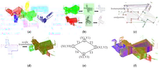
Figure 1. The pipeline of our framework. (a) Input point clouds; (b) Gaussian-weighting projection; (c) Image matching with endpoint verification; (d) Transformation between point clouds; (e) Global optimization for multi-station point cloud registration; (f) Output point clouds.

2.1. Gaussian-Weighting Projection

In this stage, we first project the original input point clouds into 2D grids to resample point clouds and simplify the neighbor searching process. For the point cloud P from each station, we first slice the original point cloud along the x-axis and y-axis to a 2D grid with the cell size of s × s as shown in Figure 2a. As the amount of point cloud data can be rather large, such as campus landscapes and large outdoor artificial buildings, the cell size is better set not to be too small, or else the following processing would be computationally intensive. In practice, s for indoor and outdoor data are set to different values, as described in Section 3.3.

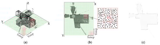
Figure 2. Point cloud projection. (a) Point cloud after 2D grid regularization; (b) 8-neighborhood weighting to calculate density; (c) Normalized to obtain grayscale image.

The point density for each cell is then calculated as shown in Figure 2b. Since there are occlusions during point cloud collection, and point clouds are often unevenly distributed, straightly using the number of points inside a cell to be its point density will produce obvious aliasing, especially when there are no points inside that cell. Another problem is that directly using the number of points inside a cell to represent the point density brings about the aliasing of the generated image. To overcome these challenges, we introduce a Gaussian-weighting function combined with neighboring cells to calculate the point density of each cell.

The Gaussian-weighting function employed to calculate the point density $\mathrm{g}\left({\mathrm{x}}_{\mathrm{c}}{,\mathrm{y}}_{\mathrm{c}}\right)$ of a cell c is as follows:

$$\mathrm{g}\left({\mathrm{x}}_{\mathrm{c}}{,\mathrm{y}}_{\mathrm{c}}\right)={\displaystyle \sum }_{\mathrm{i}=1}^{\mathrm{n}}\frac{1}{\sqrt{2\mathsf{\pi }}\mathsf{\sigma }}{\mathrm{e}}^{-\frac{1}{2}{\left(\frac{{\mathrm{d}}_{\mathrm{i}}}{\mathsf{\sigma }}\right)}^2}$$

(1)

$${\mathrm{d}}_{\mathrm{i}}=\sqrt{{\left({\mathrm{x}}_{\mathrm{i}}-{\mathrm{x}}_{\mathrm{c}}\right)}^2+{\left({\mathrm{y}}_{\mathrm{i}}-{\mathrm{y}}_{\mathrm{c}}\right)}^2}{,\mathrm{c}}_{\mathrm{i}}\mathsf{ϵ}\mathrm{g}$$

(2)

where $\left({\mathrm{x}}_{\mathrm{c}}{,\mathrm{y}}_{\mathrm{c}}\right)$ is the center coordinates of $\mathrm{c}$. ${\mathrm{d}}_{\mathrm{i}}$ is the 2D distance of the point ${\mathrm{c}}_{\mathrm{i}}$ to the center point of the cell $\mathrm{c}$. $\mathrm{g}$ denotes the collection of points inside the cell $\mathrm{c}$ and its 8 neighboring cells (Figure 2b). σ is the standard variance of the Gaussian-weighting function which indicates the smoothness of images. A larger σ suggests a smoother point density image. In order to better smooth the image while retaining the point cloud features, we take the value of σ to be half of the cell size, $\mathrm{s}/2$, considering the 3-σ principle. Equation (2) is to calculate the distance between the cell center and a point nearby, and Equation (1) assigns a weight to that nearby point based on the distance. In this case, the Gaussian function makes the nearer points more important and the farther points less important.

The grayscale image is finally generated as shown in Figure 2c, in which each pixel is corresponding to a cell after the regularization. Suppose that the x-y coordinates of the left-top cell center is ${(\mathrm{x}}_0{,\mathrm{y}}_0)$, for each pixel $(\mathrm{u},\mathrm{v})$ in the image whose corresponding cell center is $(\mathrm{x},\mathrm{y})$, we have:

$$\left(\begin{array}{c}\mathrm{u}\\ \mathrm{v}\end{array}\right)=\frac{1}{\mathrm{s}}\left[\left(\begin{array}{c}\mathrm{x}\\ \mathrm{y}\end{array}\right)-\left(\begin{array}{c}{\mathrm{x}}_0\\ {\mathrm{y}}_0\end{array}\right)\right]$$

(3)

Meanwhile, the value of each pixel in the image is normalized from the point density of its corresponding cell into the range of [0, 255], which meets the pixel scale requirement of grayscale images. The normalization formula is as follows:

$${\mathrm{I}}_{\mathrm{G}}\left(\mathrm{u},\mathrm{v}\right)=\frac{\mathrm{g}(\mathrm{x},\mathrm{y})-{\mathrm{g}}_{\min }}{{\mathrm{g}}_{\max }-{\mathrm{g}}_{\min }}\times 255$$

(4)

where $\mathrm{g}(\mathrm{x},\mathrm{y})$ is the density of each cell, ${\mathrm{g}}_{\max }$ and ${\mathrm{g}}_{\min }$ are the maximum and minimum of all the densities, and ${\mathrm{I}}_{\mathrm{G}}\left(\mathrm{u},\mathrm{v}\right)$ is the corresponding pixel value of the generated grayscale image. From Figure 2c, the cells of vertical walls are with higher point densities and thus larger pixel values, and the cells of ceilings are with relatively lower point densities and thus smaller pixel values, which indicates that the generated images have well preserved important structure clues of point clouds.

We further conduct a rotation invariance analysis to validate our consideration of the use of the neighboring cells during the calculation of point density as illustrated in Figure 3. The gray color of a pixel in Figure 3 represents the normalized point density. As illustrated in Figure 3a, we rotate the point cloud of a wall from the above to the bottom. With the consideration of the cells’ neighborhood weighting (Figure 3b), the projection of the rotated point cloud is still a straight line. And its endpoints remain the same, which suggests good invariance in terms of rotation. The 2D grid without considering neighboring cells (Figure 3c), in contrast, splits one straight line into two after the point cloud is rotated, which changes the detection of endpoints.

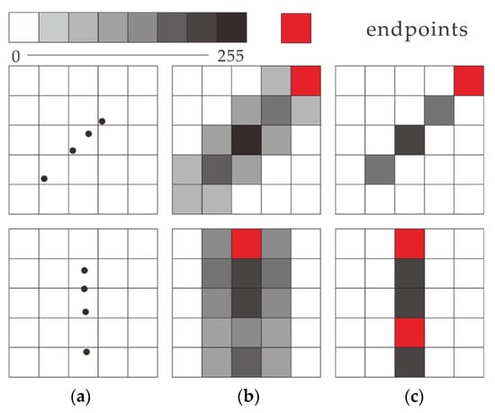
Figure 3. Rotation invariance with and without the consideration of neighboring cells. (a) Point cloud after 2D grid regularization; feature points detected in the generated images (b) with the consideration of neighboring cells and (c) without the consideration of neighboring cells.

2.2. Endpoint Validated Image Matching

In this stage, we first extract the features of generated images using SIFT and match them via a RANSAC algorithm. Then we detect endpoints to validate these matches to filter out the incorrectly matched image pairs.

2.2.1. RANSAC Image Matching

To match the generated images, we utilize SIFT to extract feature points and their descriptors, and use a RANSAC algorithm to perform feature matching in our framework. The image matching process is described as Algorithm 1.

Algorithm 1. RANSAC Image Matching.

1:  Macth (Itarget, Isource)

2:    SIFT (Itarget, Isource) →n pairs of feature points(Ftarget, Fsource)

3:    if (n < 2) return false

4:    random (i, j∈[1,n], i≠j)

5:      p1 = Ftarget.i, p2 = Ftarget.j

6:      p3 = Fsource.i, p4 = Fsource.j

7:      Trans

8:        RIM = rotation matrix (angle($\overrightarrow{\mathrm{p}1\mathrm{p}2}$, $\overrightarrow{\mathrm{p}3\mathrm{p}4}$))

9:        p3’ = RIM (p3), p4’ = RIM (p4)

10:        TIM = dist (midpoint (p1, p2), midpoint (p3’, p4’))

11:        Ts,t ← (RIM, TIM)

12:      m = num of dist (Ftarget, Ts,t (Fsource)) < threshold

13:    until mmax

14:    return Tfinal

Step 1: For the source image ${\mathrm{I}}_{\mathrm{source}}$ and target image ${\mathrm{I}}_{\mathrm{target}}$, SIFT is used to extract $\mathrm{n}$ correspondence point pairs, and if $\mathrm{n}$ is less than 2, the matching fails and exits directly.

Step 2: Two point pairs are randomly selected from the $\mathrm{n}$ pairs, and then the rotation angle $\mathsf{\theta }$ is calculated from the two pairs as shown in Figure 4a. ${\mathrm{I}}_{\mathrm{source}-\mathsf{\theta }}$ is obtained from rotating ${\mathrm{I}}_{\mathrm{source}}$ by $\mathsf{\theta }$, and the corresponding rotation matrix is:

$${\mathrm{R}}_{\mathrm{IM}}=\left(\begin{array}{cc}\cos \mathsf{\theta }& -\sin \mathsf{\theta }\\ \sin \mathsf{\theta }& \cos \mathsf{\theta }\end{array}\right)$$

(5)

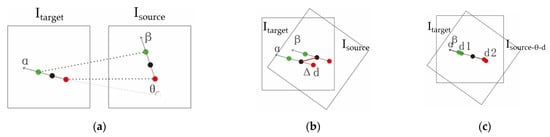
Figure 4. Image transformation: (a) Angle calculation; (b) Distance calculation after the rotation of the source image; (c) Translation of the source image.

Step 3: The average of the differences in the coordinates between points in each pair, $\Delta \mathrm{d}$, is calculated as shown in Figure 4b. Then ${\mathrm{I}}_{\mathrm{source}-\mathsf{\theta }-\mathrm{d}}$ is obtained from translating ${\mathrm{I}}_{\mathrm{source}-\mathsf{\theta }}$ by $\Delta \mathrm{d}$ as shown in Figure 4c, and the corresponding translation matrix is:

$${\mathrm{T}}_{\mathrm{IM}}=\left(\begin{array}{c}{\Delta \mathrm{d}}_{\mathrm{u}}\\ {\Delta \mathrm{d}}_{\mathrm{v}}\end{array}\right)$$

(6)

The transformation ${\mathrm{T}}_{\mathrm{s},\mathrm{t}}$ is thus the combination of the rotation and translation.

Step 4: The distance between each point pair is calculated after transforming all the feature points in ${\mathrm{I}}_{\mathrm{source}}$ by ${\mathrm{T}}_{\mathrm{s},\mathrm{t}}$. If the distance of a point pair is less than a certain threshold, it is considered as an ‘inner point’ in RANSAC. Then the number of ‘inner points’ $\mathrm{m}$ is counted.

Step 5: We repeat Steps 2–4 to obtain the transformation with the maximum number of the ‘inner points’ ${\mathrm{m}}_{\max }$, and then use the ${\mathrm{m}}_{\max }$ interior points together to calculate the final transformation matrix ${\mathrm{T}}_{\mathrm{final}}$ between images.

2.2.2. Endpoint Validation

RANSAC only performs well in image matching with reliable feature points and descriptors. However, there can still be a considerable portion of unreliable detected feature points due to tough situations such as heavy occlusions, which lowers the confidence of the RANSAC algorithm and produces unreliable image matching especially when only a few feature points are extracted. In this case, we design a method called endpoint validation to filter out the unreliable image matching, the core idea of which is to leverage the endpoints of detected line segments. In this method, we first use Hough transform, a voting algorithm in Hough parameter space, to detect line segments in grayscale images (Figure 5b). We then employ the parallelism analysis in combination with the Non-Maximum Suppression (NMS) in the Hough space to remove the unreliable lines (Figure 5c,d), since incorrectly detected line segments would be included in the detection results. Finally, we extract and match endpoints of the line segments between each two images to validate the RANSAC image matching results.

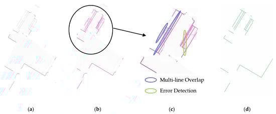
Figure 5. Line segment detection. (a) Grayscale image; (b) Line segment detection through Hough transform; (c) Illustration of incorrectly detected line segments; (d) Line segments after NMS.

Here, we first demonstrate some typical incorrect Hough transform detections as shown in Figure 5c. One is that multiple parallel line segments extremely close to each other may be detected for one wall as shown in each blue circle, and another one is false positive line segments as shown in the green circle.

Then we introduce parallelism analysis and NMS in detail to solve the aforementioned issues. In accordance with the room layout, the projections of walls on the x-y plane are parallel or perpendicular in most cases. As a result, there are groups of parallel lines in generated grayscale images. Based on this, we carry out the parallelism analysis to extract groups of lines with similar slopes. Firstly we cluster each line $\mathrm{L}$ into an existent group with the average slope $\mathsf{\phi }$ if the slope ${\vartheta }_{\mathrm{L}}$ of $\mathrm{L}$ satisfies:

$$\exists \mathsf{\phi }\in \mathsf{\varphi },\left|{\vartheta }_{\mathrm{L}}-\mathsf{\phi }\right|\le \mathsf{\tau }\left|\mathsf{\phi }\right|$$

(7)

where $\mathsf{\varphi }$ is the collection of all the average slopes of groups, and $\mathsf{\tau }$ is a small positive number close to zero. If there is no such group, we create a new one with this line $\mathrm{L}$. After the clustering of all the lines, we only keep the lines in the two largest groups for the NMS calculation.

Different from using the overlapping ratio in the object detection, we use the distance between parallel lines as the criteria in the NMS to detect lines as Algorithm 2.

Algorithm 2. NMS Line Filtering.

1:  Filter (parallel lines)

2:     collection LA (parallel lines), LF (empty)

3:     repeat

4:       l = higest voting score(LA)

5:       LA.remove(l), LF.add(l)

6:       for(l’∈LA)

7:         if(dist(l,l’) < threshold) LA.remove(l’)

8:     until LA is empty

9:     return LF

Step 1: Prepare two collections of lines $\mathrm{LA}$ and $\mathrm{LF}$. Initialize $\mathrm{LA}$ with all the detected lines after parallelism analysis, and $\mathrm{LF}$ to be empty.

Step 2. Take the line $\mathrm{l}$ with the highest voting score from the remaining lines in $\mathrm{LA}$, remove it from $\mathrm{LA}$ and add it to $\mathrm{LF}$.

Step 3. Calculate the distance of line $\mathrm{l}$ to each line $\mathrm{l}\text{’}$ in $\mathrm{LA}$. If the distance is smaller than the threshold ${\mathrm{d}}_{\mathrm{t}}$, remove that line $\mathrm{l}’$ from $\mathrm{LA}$.

Step 4. Repeat Steps 2–3 until there are no more lines left in $\mathrm{LA}$. $\mathrm{LF}$ is the final collection of detected lines as shown in Figure 5d.

Subsequently, we obtain the endpoints including the ends of the detected line segments and the wall corner points, i.e., the intersection points from extending those line segments. As illustrated in Figure 6a, the red points are the endpoints extracted in image ${\mathrm{I}}_{\mathrm{target}}$, and the green ones are those in image ${\mathrm{I}}_{\mathrm{source}}$. After applying the transformation matrix ${\mathrm{T}}_{\mathrm{final}}$ calculated in Section 2.2.1 to the endpoints of ${\mathrm{I}}_{\mathrm{source}}$, we calculate the distance between each red endpoint and each transformed green endpoint. If the distance is less than a threshold (usually two pixels), these two endpoints are considered to be matched. If less than two pairs of endpoints are matched, the match of these two images is invalid and filtered out.

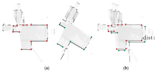
Figure 6. Verify the matching using endpoints. (a) Endpoint detection; (b) Endpoint matching.

2.3. Point Cloud Transformation

In this section, we aim to calculate the transformation between each two point clouds from the image transformation obtained in Section 2.2. Suppose that ${\mathrm{I}}_{\mathrm{i}}$ and ${\mathrm{I}}_{\mathrm{j}}$ are the generated grayscale images of point clouds ${\mathrm{P}}_{\mathrm{i}}$ and ${\mathrm{P}}_{\mathrm{j}}$, the transformation of ${\mathrm{I}}_{\mathrm{i}}$ into the coordinate system of ${\mathrm{I}}_{\mathrm{j}}$ is as follows:

$$\left(\begin{array}{c}{\mathrm{u}}_{\mathrm{j}}\\ {\mathrm{v}}_{\mathrm{j}}\end{array}\right){=\mathrm{R}}_{\mathrm{IM}}\left(\begin{array}{c}{\mathrm{u}}_{\mathrm{i}}\\ {\mathrm{v}}_{\mathrm{i}}\end{array}\right){+\mathrm{T}}_{\mathrm{IM}}$$

(8)

where ${\mathrm{R}}_{\mathrm{IM}}$ and ${\mathrm{T}}_{\mathrm{IM}}$ (expressed in Equations (5) and (6)) are the rotation and translation matrix from ${\mathrm{T}}_{\mathrm{final}}$ respectively, and $\left({\mathrm{u}}_{\mathrm{i}}{,\mathrm{v}}_{\mathrm{i}}\right)$ is a pixel in ${\mathrm{I}}_{\mathrm{i}}$, and $\left({\mathrm{u}}_{\mathrm{j}}{,\mathrm{v}}_{\mathrm{j}}\right)$ is the transformed pixel of $\left({\mathrm{u}}_{\mathrm{i}}{,\mathrm{v}}_{\mathrm{i}}\right)$ in the coordinate system of ${\mathrm{I}}_{\mathrm{j}}$.

According to Equation (3), there is a scaling and translation relation between an image and its corresponding point cloud, and thus the transformations from ${\mathrm{P}}_{\mathrm{i}}$ to ${\mathrm{I}}_{\mathrm{i}}$ and ${\mathrm{P}}_{\mathrm{j}}$ to ${\mathrm{I}}_{\mathrm{j}}$ are as follows:

$$\left(\begin{array}{c}{\mathrm{u}}_{\mathrm{i}}\\ {\mathrm{v}}_{\mathrm{i}}\end{array}\right)=\frac{1}{\mathrm{s}}\left[\left(\begin{array}{c}{\mathrm{x}}_{\mathrm{i}}\\ {\mathrm{y}}_{\mathrm{i}}\end{array}\right)-\left(\begin{array}{c}{\mathrm{x}}_{\mathrm{i}0}\\ {\mathrm{y}}_{\mathrm{i}0}\end{array}\right)\right]$$

(9)

$$\left(\begin{array}{c}{\mathrm{u}}_{\mathrm{j}}\\ {\mathrm{v}}_{\mathrm{j}}\end{array}\right)=\frac{1}{\mathrm{s}}\left[\left(\begin{array}{c}{\mathrm{x}}_{\mathrm{j}}\\ {\mathrm{y}}_{\mathrm{j}}\end{array}\right)-\left(\begin{array}{c}{\mathrm{x}}_{\mathrm{j}0}\\ {\mathrm{y}}_{\mathrm{j}0}\end{array}\right)\right]$$

(10)

Combining Equations (8)–(10), we deduce the transformation of ${\mathrm{P}}_{\mathrm{i}}$ into the coordinate system of ${\mathrm{P}}_{\mathrm{j}}$ as Equation (11). The transformation is further refined by using the ICP algorithm.

$$\left(\begin{array}{c}{\mathrm{x}}_{\mathrm{j}}\\ {\mathrm{y}}_{\mathrm{j}}\end{array}\right)=\left(\begin{array}{cc}\cos \mathsf{\theta }& -\sin \mathsf{\theta }\\ \sin \mathsf{\theta }& \cos \mathsf{\theta }\end{array}\right)\left(\begin{array}{c}{\mathrm{x}}_{\mathrm{i}}{-\mathrm{x}}_{\mathrm{i}0}\\ {\mathrm{y}}_{\mathrm{i}}{-\mathrm{y}}_{\mathrm{i}0}\end{array}\right)+\left(\begin{array}{c}{\mathrm{x}}_{\mathrm{j}0}\\ {\mathrm{y}}_{\mathrm{j}0}\end{array}\right)+\mathrm{s}\left(\begin{array}{c}{\Delta \mathrm{d}}_{\mathrm{u}}\\ {\Delta \mathrm{d}}_{\mathrm{v}}\end{array}\right)$$

(11)

2.4. Global Least-Square Optimization

In this section, we aim to calculate a base coordinate system where all the point clouds are registered to. A simple way to handle this is to select one of the clouds as the base, and then directly register other clouds to this base. The transformation between a cloud and the base can be obtained from the precalculated station-by-statin transformation. The problem of this way is that when the transformation chain is very long, there will be a large accumulation error. To resolve this problem, we introduce a global least-square optimization method to minimize the overall error.

As shown in Figure 7, we first construct a graph, where each node represents the transformation ${\mathrm{T}}_{\mathrm{i}}$ from the base coordinate system to a point cloud ${\mathrm{P}}_{\mathrm{i}}$ that we need to calculate, and each edge represents the transformation ${\mathrm{T}}_{\mathrm{i},\mathrm{j}}$ from ${\mathrm{P}}_{\mathrm{i}}$ to ${\mathrm{P}}_{\mathrm{j}}$. Thus, the transformation ${\mathrm{T}}_{\mathrm{i},\mathrm{j}}$ can be expressed as:

$${\mathrm{T}}_{\mathrm{i},\mathrm{j}}{=\mathrm{T}}_{\mathrm{i}}^{-1}{\mathrm{T}}_{\mathrm{j}},$$

(12)

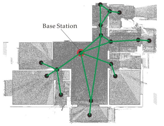
Figure 7. Multi-station cloud global optimization schematic.

In this graph, the values of edges are known from the calculation in the above sections, and the values of the nodes need to be derived. The deviation between the known and derived values can thus be expressed by transforming Equation (12) as follows:

$${\mathrm{e}}_{\mathrm{i},\mathrm{j}}{=\mathrm{T}}_{\mathrm{i},\mathrm{j}}^{-1}{\mathrm{T}}_{\mathrm{i}}^{-1}{\mathrm{T}}_{\mathrm{j}},$$

(13)

where ${\mathrm{e}}_{\mathrm{i},\mathrm{j}}$ is a matrix whose deviation from the identity matrix indicates the error.

An energy function is designed for all point clouds:

$$\mathrm{E}=\frac{1}{2}{{\displaystyle \sum }}_{\mathrm{i},\mathrm{j}}{\mathrm{e}}_{\mathrm{i},\mathrm{j}}^{\mathrm{T}}{\mathsf{\Sigma }}_{\mathrm{ij}}^{-1}{\mathrm{e}}_{\mathrm{i},\mathrm{j}},$$

(14)

where ${\mathsf{\Sigma }}_{\mathrm{ij}}^{-1}$ is the information matrix representing the importance of the edge $⟨\mathrm{i},\mathrm{j}⟩$.

At the beginning of the optimization, we use a base station as the initialization of the base coordinate system. The base station is the node in the graph with the most connections to other nodes in Figure 7. Then we minimize the energy in Equation (14) by using the Levenberg-Marquardt method from a graph optimization library named g2o. As the final result, we transform all the point clouds based on the optimized matrices to obtain a complete model.

3. Results

3.1. Dataset

In this paper, we utilize six terrestrial point cloud datasets to validate the performance of our framework. They are IPSN-2016, IPSN-2017, WHU-CAM, WHU-RES, WHUT-WK and WHUT-BSZ datasets, which includes four benchmark datasets and two datasets collected by ourselves. These point cloud datasets were collected in four large indoor scenes and two outdoor scenes.

A. IPSN-2016 and IPSN-2017. As shown in Figure 8, both two datasets are from the Microsoft Indoor Positioning Competition. IPSN-2016 was collected in a two-level exhibition area with 26 stations and 6,489,573 points. There is an up-and-down roof in this exhibition area. IPSN-2017 was collected with 47 stations and 4,624,991 points in a similar building scene but with a flat roof. These two datasets were collected in large indoor buildings with complex structures.

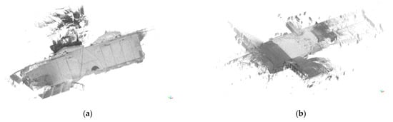
Figure 8. (a) IPSN-2016 and (b) IPSN-2017.

B. WHU-CAM and WHU-RES. As shown in Figure 9, these two datasets were collected at Wuhan University including high-rise buildings, metro stations, tunnels and other artificial structures. Alignment experiments are conducted on the datasets collected in the campus and residence area. The campus has 10 stations and 301,908 points, and the residence has 7 stations and 308,145 points. Both two datasets were collected in outdoor scenes. Compared to indoor point clouds, outdoor point cloud registration is more challenging, since buildings might be heavily occluded by trees in outdoor scenes.

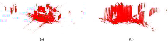
Figure 9. (a) WHU-CAM and (b) WHU-RES.

C. WHUT-WK and WHUT-BSZ. As shown in Figure 10, except for the above four benchmark datasets, we collected another two indoor terrestrial point cloud datasets, WHUT-WK and WHUT-BSZ, at Wuhan University of Technology. WHUT-WK was collected with 19 stations and 580,315 points, and WHUT-BSZ was collected with 11 stations and 1,749,584 points. Compared to the other four public datasets, these two datasets have a smaller amount of point cloud data, more complex indoor structures and lower overlapping areas between adjacent stations. These features make multi-station point cloud registration more challenging.

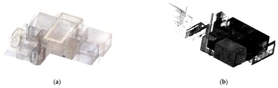
Figure 10. (a) WHUT-WK and (b) WHUT-BSZ.

3.2. Evaluation Metrics

In this experiment, two metrics are utilized for the evaluation of the performance of our framework. They are the rotation invariance of feature points in the images generated from the projection of point clouds, the accuracy and the efficiency of point cloud registration. We realize our algorithm by C++ in Visual Studio and run our code on a 64-bit Windows 10 mobile workstation with Intel Core i7-8750H@ 2.20 GHz and 8G RAM.

3.2.1. Rotation Invariance of Gaussian-Weighting Projection

The image matching process in this paper requires our Gaussian-weighting projection to be rotation invariant, so that the correspondence images pairs could be robustly matched. To evaluate the rotation invariance of Gaussian-weighting projection, we utilize the repetition rate, i.e., the reproducible ability of detecting feature points at the same location, as the metric.

Suppose that a grayscale image ${\mathrm{I}}_0$ is obtained from the projection of a point cloud ${\mathrm{P}}_0$, and feature points $\left\{{\mathrm{f}}_1,{\mathrm{f}}_2\cdots \right\}$ are extracted from ${\mathrm{I}}_0$ by using SIFT features. The point cloud ${\mathrm{P}}_0$ is then rotated by an angle $\mathsf{\theta }$ to obtain the point cloud ${\mathrm{P}}_{\mathsf{\theta }}$. Similarly, feature points $\left\{{\mathrm{f}}_1^{\mathsf{\theta }},{\mathrm{f}}_2^{\mathsf{\theta }}\cdots \right\}$ are detected in the generated image ${\mathrm{I}}_{\mathsf{\theta }}$ from ${\mathrm{P}}_{\mathsf{\theta }}$. Then the feature points $\left\{{\mathrm{f}}_1^{\mathsf{\theta }},{\mathrm{f}}_2^{\mathsf{\theta }}\cdots \right\}$ are rotated back by $-\mathsf{\theta }$ with a transformation matrix T to obtain $\left\{\mathrm{T}{\mathrm{f}}_1^{\mathsf{\theta }},\mathrm{T}{\mathrm{f}}_2^{\mathsf{\theta }}\cdots \right\}$. Correspondence point pairs are validated by calculating the distance between $\mathrm{T}{\mathrm{f}}_{\mathrm{i}}^{\mathsf{\theta }}$ and ${\mathrm{f}}_{\mathrm{j}}$. If the distance is less than a threshold value $\mathsf{ϵ}$ (set to be two pixels in our experiments), ${\mathrm{f}}_{\mathrm{j}}$ is considered a rotationally invariant feature point. The whole process is shown in Figure 11. The rotation invariant of a feature point ${\mathrm{f}}_{\mathrm{j}}$ is justified as follows:

$$\mathrm{invariance}=\{\begin{array}{c}\begin{array}{c}1,\mathrm{if}\left||{\mathrm{Tf}}_{\mathrm{i}}^{\mathsf{\theta }}{-\mathrm{f}}_{\mathrm{j}}|\right|\le \mathsf{ϵ}\\ 0,\mathrm{if}\left||{\mathrm{Tf}}_{\mathrm{i}}^{\mathsf{\theta }}{-\mathrm{f}}_{\mathrm{j}}|\right|>\mathsf{ϵ}\end{array}\end{array},$$

(15)

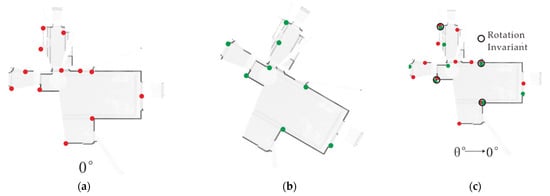
Figure 11. Rotation invariance of the generated image. (a) Detected SIFT feature points on image ${\mathrm{I}}_0$; (b) Detected SIFT feature points on image ${\mathrm{I}}_{\mathsf{\theta }}$; (c) The rotation invariant feature point validation.

The repetition rate is as follows:

$$\mathrm{Repeatability}=\frac{{\mathrm{N}}_{\mathrm{Inv}}}{{\mathrm{N}}_{\mathrm{All}}},$$

(16)

where ${\mathrm{N}}_{\mathrm{Inv}}$ is the number of rotation-invariant feature points, and $\mathrm{n}$ is the number of all feature points detected from the image ${\mathrm{I}}_0$.

3.2.2. Accuracy and Efficiency of Point Cloud Registration

We evaluate the registration accuracy by computing the root mean square error (RMSE) between the registered terrestrial point cloud with the ground truth data. In this experiment, the ground truth point cloud is obtained from manually registering point clouds, the same input point clouds of our framework. The RMSE is calculated as follows:

$$\mathrm{RMSE}=\sqrt{\frac{1}{\mathrm{n}}{\displaystyle \sum }_{\mathrm{i}=1}^{\mathrm{n}}\left[{\left({\mathrm{x}}_{\mathrm{i}}{-\mathrm{x}}_{\mathrm{i}}^{\prime }\right)}^2+{\left({\mathrm{y}}_{\mathrm{i}}{-\mathrm{y}}_{\mathrm{i}}^{\prime }\right)}^2+{\left({\mathrm{z}}_{\mathrm{i}}{-\mathrm{z}}_{\mathrm{i}}^{\prime }\right)}^2\right]}$$

(17)

where n is the total number of points in the registered point cloud, (${\mathrm{x}}_{\mathrm{i}},{\mathrm{y}}_{\mathrm{i}},{\mathrm{z}}_{\mathrm{i}}$) is the coordinate of a point from the ground truth point cloud, and (${\mathrm{x}}_{\mathrm{i}}^{\prime },{\mathrm{y}}_{\mathrm{i}}^{\prime },{\mathrm{z}}_{\mathrm{i}}^{\prime }$) is the coordinate of a point from the registered point cloud.

Moreover, we measure the efficiency of our method by recording the whole processing time from the projection of the point clouds to the global optimization.

3.3. Parameter Analysis

To explore the effect of cell size, we conduct two sets of experiments on the indoor and the outdoor dataset to test the efficiency and accuracy respectively. Rather than register multi-station point clouds, we register point clouds station-by-station from each dataset as a group test in the experiments. There are six groups of tests in indoor datasets and four groups in outdoor datasets. As illustrated in Figure 12, the size of the generated image decreases with the increase in cell size, and thus less feature points are detected. Consequently, a small number of feature points may even cause images not matched. For instance, in WHUT-WK, the performance is getting worse from a cell size larger than 0.07 m. In the indoor datasets, there are four groups with similar accuracy, of which the cell size is in the range of 0.01–0.06 m. When the cell size is above 0.06 m, the accuracy starts to drop remarkably. The accuracy of the other two groups shows similar trend at 0.05 m and 0.06 m respectively. The computation time of six groups from indoor datasets starts to converge from the cell size of 0.04 m. To leverage the efficiency and accuracy, we set the range of cell size in the range of 0.03–0.06 m for the indoor datasets. For the outdoor datasets, the accuracy does not change significantly when the cell size is in the range of 0.1–1.6 m. Additionally, there is no significant change with the computation time when the cell size is in the range of 0.7–2.5 m. To keep a decent trade-off between efficiency and accuracy, we set the range of cell size in the range of 0.7–1.6 m for the outdoor datasets.

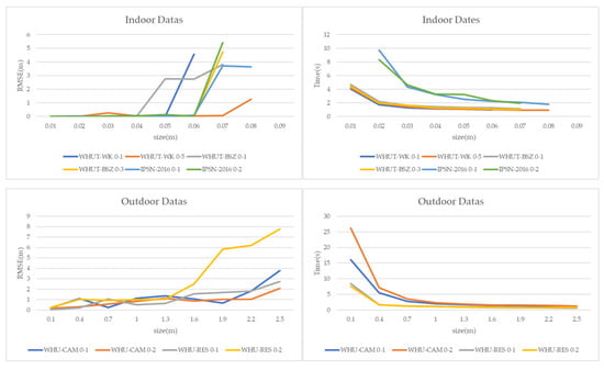
Figure 12. The effect of cell size on registration accuracy and time. The larger the cell size is, the smaller the generated image will be, accompanied by faster registration speed and worse accuracy.

3.4. Performance Analysis

3.4.1. Superiority Gaussian-Weighting Projection

In this section, we compare the rotation invariance of feature points in grayscale images generated by different point cloud projection strategies to prove the superiority of Gaussian-weighting projection. We conduct experiments on four datasets (WHUT-WK, WHUT-BSZ, IPSN-2016 and WHU-CAM). In the experiment, we first obtain 36 new point clouds by rotating the original point cloud 36 times with a 10° interval. Then we generate grayscale images using five different point cloud projection methods and detect feature points using SIFT afterwards. The five methods include 1 × 1, 3 × 3, and 5 × 5 neighborhood-weighting, binary mapping and unweighted projection methods. The average repetition rate is calculated for each point cloud in the four datasets.

The average repetition rates of five projection methods on four datasets are shown in Table 1. In terms of the rotation invariance, the 3 × 3 neighborhood weighting method performs the best, with an average value of 0.584 for the four datasets. The 5 × 5 neighborhood weighting is the second best, with an average value of 0.577. Compared to the 3 × 3, the 5 × 5 is more time-consuming. The reason is that the use of neighborhood-weighting well preserves the geometric features of point clouds and is robust to occlusion, which is as analyzed in Section 2.1. The binary mapping is able to obtain decent results with an average repetition rate of 0.556. It is because the binary mapping is not able to distinguish the differences of density and thus less stable. For instance, there are large fluctuations in the IPSN-2016 data as shown in Figure 13. In contrast, the 1 × 1 and unweighted methods perform worse, since these two methods could be easily affected by the sparse point cloud and occluded scenes, as indicated in Section 2.2.

Table 1. Average Repetition Rate of Different Projection Methods.

	Method	5 × 5 Neighbor	3 × 3 Neighbor	1 × 1 Neighbor	Binary Image	Unweighted
Datasets
WHUT-WK(avg)		0.635	0.658	0.325	0.600	0.332
WHUT-BSZ(avg)		0.625	0.604	0.339	0.589	0.294
IPSN-2016(avg)		0.565	0.568	0.241	0.553	0.246
WHU-CAM (avg)		0.481	0.504	0.230	0.483	0.192
AVG of all datasets		0.577	0.584	0.284	0.556	0.266

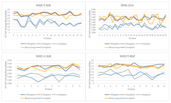
Figure 13. Comparison of rotation invariance of different projection methods.

3.4.2. Two-Station Cloud Alignment Performance

In this section, we compare the efficiency and accuracy of our framework to other 3D point cloud registration methods, including 4PCS [11], super-4PCS [12], k-4PCS [14] and Sánchez-Belenguer’s method [33]. In the experiment, we perform the station-by-station point cloud registration on the indoor dataset WHUT-WK and the outdoor dataset WHU-CAM as illustrated in Figure 14. Our registration time of two-station point clouds on the indoor datasets is between 1 and 1.5 s, and on the outdoor datasets is in the range of 5–7.5 s, which is comparable to Sánchez-Belenguer’s method, and much smaller than 4PCS based methods. Furthermore, our method achieves the RMSE of 0.118 m for 10 sets of indoor point clouds and 1.11 m for 10 sets of outdoor point clouds. In terms of the average RMSE of registering indoor data, our framework is 12.63 times better than 4PCS, 8.02 times better than super-4PCS, 6.02 times better than k-4PCS, and 2.82 times better on the indoor dataset and 1.46 times better on the outdoor dataset than Sánchez-Belenguer’s method.

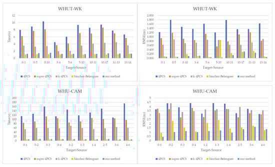
Figure 14. The comparison of efficiency and accuracy.

Projection-based methods significantly outperform other 3D point cloud registration methods for both efficiency and accuracy. For efficiency, the projection-based methods only search feature points in images instead of traversing every point in 3D point clouds to find correspondences between point clouds, which thus greatly improves the efficiency of registration. Moreover, the processing time of the projection-based methods is much less affected by the number of points in each cloud. As for accuracy, projection-based methods are at least 2 times better than other methods in terms of the average RMSE of registering outdoor data.

Compared to Sánchez-Belenguer’s point cloud projection method, our method consumes a bit more time since the neighborhood weighting takes into account more cells for the calculation. Whereas benefiting from Gaussian-weighting projection, our method is ~2 times better than Sánchez-Belenguer’s method in terms of accuracy.

3.5. Ablation Study

In addition, we test the performance of our framework on multi-station point clouds and conduct the ablation study on the aforementioned six datasets to evaluate two modules, global optimization and endpoint validation. As illustrated in Table 2, our framework with global optimization and endpoint validation performs the best. The framework without global optimization and endpoint performs the worst. The other two frameworks, with only global optimization or with only endpoint validation, perform the second best. The accuracy of three experimental datasets shows great improvement with the endpoint validation module, which indicates that our endpoint validation significantly filters out negative image matches. And the improvement of accuracy on all datasets using global optimization suggests that our global optimization module has greatly improved the overall accuracy of multi-station point cloud registration.

Table 2. Comparison of endpoint validation, global optimization. GO and NGO means with and without global optimization, and EV and NEV means with and without endpoint validation, respectively.

Datasets (Number of Stations)	Average Error (m)/Number of Alignment Stations
	NGO + NEV	NGO + EV	GO + NEV	GO + EV
WHUT-WK (19)	5.35/19	0.06/10	4.21/19	0.04/10
WHUT-BSZ (12)	0.10/12	0.10/12	0.09/12	0.09/12
IPSN-2016 (26)	3.30/24	0.11/21	2.61/24	0.08/21
IPSN-2017 (47)	1.86/47	1.23/43	1.57/47	0.98/43
WHU-CAM (10)	1.08/10	1.08/10	1.04/10	1.04/10
WHU-RES (7)	0.25/6	0.25/6	0.23/6	0.23/6

As shown in Figure 15 and Figure 16, we analyze the endpoint validation on WHUT-WK. In Figure 15, there are two station-connectivity diagrams, which illustrates the matching relations between two stations. In each diagram the green cells with number 1 indicates that the two stations are matched, and the pink cells represents the filtered out incorrectly matched stations. Empty cells illustrate that there is no connectivity between the two stations. Before the endpoint validation processing, station 2 is connected to station 3, and station 3 is connected to stations 5 and 8. Station 12 is connected to station 14, and station 11 is connected to station 15. After the endpoint validation, the matching relation of these stations are filtered out. The endpoint validation method effectively filters out incorrect matches. As shown in Figure 16, there is no overlapping between stations 12 and 14. Without endpoint validation the framework obtains an incorrect matching relation between stations 12 and 14. After endpoint validation, the negative match is filtered out. Station 3 and 5 are roughly registered due to the close distance between SIFT feature points. Even though stations 11 and 15 have a large overlap rate, they are still incorrectly matched. This is because the SIFT does not detect enough features in simple structured indoor scenes.

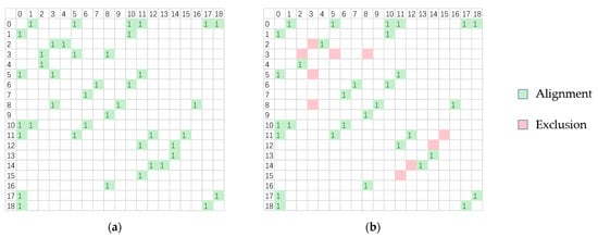
Figure 15. WHUT-WK alignment connectivity diagram. (a) Without endpoint verification. (b) With endpoint verification.

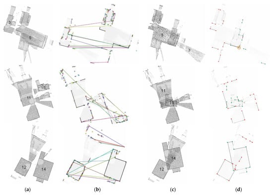
Figure 16. The filtering of incorrect matching on WHUT-WK. (a) Initial location. (b) Feature point matching. (c) Incorrect results. (d) Endpoint validation.

With the endpoint validation and global optimization, our framework significantly improves the terrestrial point cloud registration. The qualitative registration results of six datasets are shown in Figure 17.

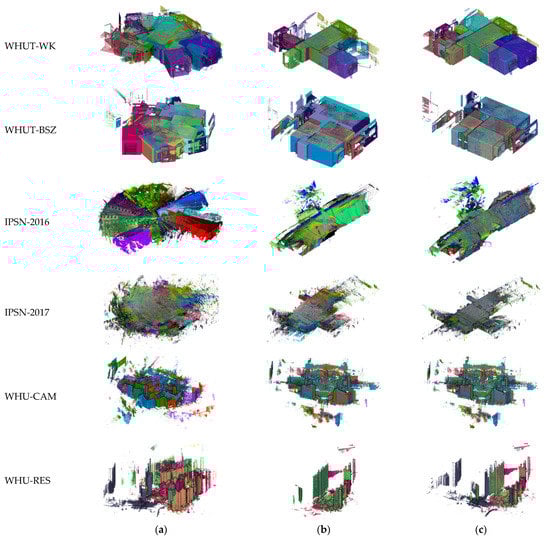
Figure 17. Global alignment results. (a) Input point clouds. (b) Alignment results. (c) Ground truth.

4. Discussion

Point cloud registration algorithms based on spatial feature points need to find and describe the feature points in 3D space, which is indeed beneficial for the registration of various angular positions. However, experiments have shown that the efficiency of the traditional spatial point cloud alignment method is lower for point cloud data of buildings collected in plane and automatically leveled, as the characteristics of such point clouds are not taken into account. At the same time, the spatial features need to consider the transformation of 6 degrees of freedom, which is more complicated in terms of formulation. In this paper, we use a point cloud alignment method based on image matching, which has a good improvement in efficiency and a relatively simple formulation. Experiment 3.4.2 shows that our method has a 2–12 times improvement in efficiency compared to spatial point cloud alignment algorithms.

For the projection of point clouds into images, the 2D grid regularization step is prone to bring about aliasing effects. In order to solve this problem and to make the resulting images more stable in terms of rotational invariance, we use a domain weighting method to smooth out the aliasing. Experiment 3.4.1 shows that the use of domain weighting results in more stable rotationally invariant feature points.

For image matching, which we based on the SIFT algorithm, although the method has good rotational invariance as well as maintaining a degree of stability to scale scaling and noise as well, there is still mismatching, which cannot exist in global alignment of multi-site clouds. We build on this algorithm by obtaining line segment endpoints and intersections through straight line detection and using the overlap of the transformed endpoints and intersections to verify the correctness of the matches, which can rule out incorrect matches well. The results of Experiment 3.5 show that our method is able to significantly reduce the global alignment error after excluding some of the unmatched data.

5. Conclusions

This paper proposes a terrestrial point cloud registration framework based on Gaussian-weighted projected image matching. In our framework, we first project terrestrial point clouds into 2D grids and generate grayscale images based on our Gaussian-weighting function. We then use the SIFT and RANSAC algorithm to perform image matching, after which endpoints are extracted to filter out incorrect matches. Subsequently, we calculate the transformation relation between point clouds station-by-station. We finally align multi-station point clouds by a global least-square optimization, and then obtain the complete model. Experimental results indicate that our Gaussian-weighting projection is rotation invariant and well preserves the structure information of terrestrial point clouds, and our endpoint validation method effectively filters out incorrect matches between images. In summary, our framework greatly outperforms other methods and achieves the state-of-the-art performance. A limitation of our framework might be that the point clouds must be collected for a scene with a flat plane. Our future work will focus on the registration of terrestrial point clouds in irregular building scenes.

References

- Tam, G.K.; Cheng, Z.Q.; Lai, Y.K.; Langbein, F.C.; Liu, Y.; Marshall, D.; Martin, R.R.; Sun, X.F.; Rosin, P.L. Registration of 3D point clouds and meshes: A survey from rigid to nonrigid. IEEE Trans. Vis. Comput. Graph. 2012, 19, 1199–1217. [Google Scholar] [CrossRef] [PubMed] [Green Version]
- Akca, D. Full Automatic Registration of Laser Scanner Points Clouds. Ph.D. Thesis, ETH Zurich, Zurich, Switzerland, 2003. [Google Scholar]
- Al-Durgham, K.; Habib, A.; Kwak, E. RANSAC approach for automated registration of terrestrial laser scans using linear features. In Proceedings of the ISPRS Annals of the Photogrammetry, Remote Sensing and Spatial Information Sciences, Antalya, Turkey, 11–13 November 2013. [Google Scholar]
- Kang, Z.; Li, J.; Zhang, L.; Zhao, Q.; Zlatanova, S. Automatic registration of terrestrial laser scanning point clouds using panoramic reflectance images. Sensors 2009, 9, 2621–2646. [Google Scholar] [CrossRef] [PubMed] [Green Version]
- Kawashima, K.; Yamanishi, S.; Kanai, S.; Date, H. Finding the next-best scanner position for as-built modelling of piping systems. In Proceedings of the International Archives of Photogrammetry, Remote Sensing and Spatial Information Sciences, Riva Del Garda, Italy, 23–25 June 2014. [Google Scholar]
- Besl, P.J.; McKay, N.D. A method for registration of 3-D shapes. IEEE Trans. Patt. Anal. Mach. Intell. 1992, 14, 239–256. [Google Scholar] [CrossRef]
- Frome, A.; Huber, D.; Kolluri, R.; Bülow, T.; Malik, J. Recognizing objects in range data using regional point descriptors. In Proceedings of the European Conference on Computer Vision, Prague, Czech Republic, 11–14 May 2004. [Google Scholar]
- Rusu, R.B.; Blodow, N.; Marton, Z.C.; Beetz, M. Aligning point cloud views using persistent feature histograms. In Proceedings of the IEEE/RSJ International Conference on Intelligent Robots and Systems, Nice, France, 22–26 September 2008. [Google Scholar]
- Rusu, R.B.; Blodow, N.; Beetz, M. Fast point feature histograms (FPFH) for 3D registration. In Proceedings of the IEEE International Conference on Robotics and Automation, Kobe, Japan, 12–17 May 2009. [Google Scholar]
- Rusu, R.B.; Bradski, G.; Thibaux, R.; Hsu, J. Fast 3d recognition and pose using the viewpoint feature histogram. In Proceedings of the IEEE/RSJ International Conference on Intelligent Robots and Systems, Taipei, Taiwan, 18–22 October 2010. [Google Scholar]
- Aiger, D.; Mitra, N.J.; Cohen-Or, D. 4-Points Congruent Sets for Robust Pairwise Surface Registration; ACM: New York, NY, USA, 2008; p. 85. [Google Scholar]
- Mellado, N.; Aiger, D.; Mitra, N.J. Super 4pcs fast global pointcloud registration via smart indexing. Comput. Graph. Forum. 2014, 33, 205–215. [Google Scholar] [CrossRef] [Green Version]
- Mohamad, M.; Rappaport, D.; Greenspan, M. Generalized 4-points congruent sets for 3d registration. In Proceedings of the 2014 International Conference on 3D Vision, Tokyo, Japan, 8–11 December 2014. [Google Scholar]
- Theiler, P.W.; Wegner, J.D.; Schindler, K. Markerless point cloud registration with keypoint-based 4-points congruent sets. In Proceedings of the ISPRS Annals of the Photogrammetry, Remote Sensing and Spatial Information Sciences, Antalya, Turkey, 11–13 November 2013. [Google Scholar]
- Zhong, Y. Intrinsic shape signatures: A shape descriptor for 3D object recognition. In Proceedings of the IEEE International Conference on Computer Vision Workshops, ICCV Workshops 2009, Kyoto, Japan, 27 September–4 October 2009. [Google Scholar]
- Alshawa, M. ICL: Iterative closest line A novel point cloud registration algorithm based on linear features. Ekscentar 2007, 10, 53–59. [Google Scholar]
- Lindeberg, T. Scale Invariant Feature Transform. Scholarpedia 2012, 7, 10491. [Google Scholar] [CrossRef]
- Lowe, D.G. Distinctive image features from scale-invariant keypoints. Int. J. Comput. Vis. 2004, 60, 91–110. [Google Scholar] [CrossRef]
- Lowe, D.G. Object recognition from local scale-invariant features. In Proceedings of the IEEE International Conference on Computer Vision, Kerkyra, Greece, 20–25 September 1999. [Google Scholar]
- Sipiran, I.; Bustos, B. Harris 3D: A robust extension of the Harris operator for interest point detection on 3D meshes. Vis. Comput. 2011, 27, 963–976. [Google Scholar] [CrossRef]
- Harris, C.; Stephens, M. A combined corner and edge detector. In Proceedings of the Alvey Vision Conference, Manchester, UK, 31 August–2 September 1988. [Google Scholar]
- Yew, Z.J.; Lee, G.H. 3dfeat-net: Weakly supervised local 3d features for point cloud registration. In Proceedings of the European Conference on Computer Vision, Munich, Germany, 8–14 September 2018. [Google Scholar]
- Aoki, Y.; Goforth, H.; Srivatsan, R.A.; Lucey, S. Pointnetlk: Robust & efficient point cloud registration using pointnet. In Proceedings of the IEEE Conference on Computer Vision and Pattern Recognition, Long Beach, CA, USA, 15–20 June 2019. [Google Scholar]
- Qi, C.R.; Yi, L.; Su, H.; Guibas, L.J. PointNet++: Deep Hierarchical Feature Learning on Point Sets in a Metric Space. In Proceedings of the Advances in Neural Information Processing Systems, Long Beach, CA, USA, 4–9 December 2017. [Google Scholar]
- Wu, W.; Zhang, Y.; Wang, D.; Lei, Y. SK-Net: Deep learning on point cloud via end-to-end discovery of spatial keypoints. In Proceedings of the AAAI Conference on Artificial Intelligence, New York, NY, USA, 7–12 February 2017. [Google Scholar]
- Wang, Y.; Solomon, J.M. Deep closest point: Learning representations for point cloud registration. In Proceedings of the IEEE/CVF International Conference on Computer Vision, Seoul, Korea, 27 October–2 November 2019. [Google Scholar]
- Xiao, J.; Adler, B.; Zhang, H. 3D point cloud registration based on planar surfaces. In Proceedings of the IEEE International Conference on Multisensor Fusion and Integration for Intelligent Systems, Hamburg, Germany, 13–15 September 2012. [Google Scholar]
- Forstner, W.; Khoshelham, K. Efficient and accurate registration of point clouds with plane to plane correspondences. In Proceedings of the IEEE International Conference on Computer Vision Workshops, Venice, Italy, 22–29 October 2017. [Google Scholar]
- Xiao, J.; Adler, B.; Zhang, J.; Zhang, H. Planar Segment Based Three-dimensional Point Cloud Registration in Outdoor Environments. J. Field Robot. 2013, 30, 552–582. [Google Scholar] [CrossRef]
- Xu, Y.; Boerner, R.; Yao, W.; Hoegner, L.; Stilla, U. Pairwise coarse registration of point clouds in urban scenes using voxel-based 4-planes congruent sets. ISPRS J. Photogramm. Remote Sens. 2019, 151, 106–123. [Google Scholar] [CrossRef]
- Yang, B.; Dong, Z.; Liang, F.; Liu, Y. Automatic registration of large-scale urban scene point clouds based on semantic feature points. ISPRS J. Photogramm. Remote Sens. 2016, 113, 43–58. [Google Scholar] [CrossRef]
- Sumi, T.; Date, H.; Kanai, S. Multiple TLS point cloud registration based on point projection images. In Proceedings of the International Archives of Photogrammetry, Remote Sensing and Spatial Information Sciences, Riva del Garda, Italy, 4–7 June 2018. [Google Scholar]
- Sánchez-Belenguer, C.; Ceriani, S.; Taddei, P.; Wolfart, E.; Sequeira, V. Global matching of point clouds for scan registration and loop detection. Rob. Auton. Syst. 2020, 123, 103324. [Google Scholar] [CrossRef]
- Shi, J. Good Features to Track. In Proceedings of the IEEE Conference on Computer Vision Pattern Recognition, Seattle, WA, USA, 21–23 June 1994. [Google Scholar]
- Li, Z.; Zhang, X.; Tan, J.; Liu, H. Pairwise Coarse Registration of Indoor Point Clouds Using 2D Line Features. ISPRS Int. J. Geo-Inf. 2021, 10, 26. [Google Scholar] [CrossRef]
- Wang, Y.; Zheng, N.; Bian, Z. A Closed-Form Solution to Planar Feature-Based Registration of LiDAR Point Clouds. ISPRS Int. J. Geo-Inf. 2021, 10, 435. [Google Scholar] [CrossRef]
- Ge, X.; Hu, H. Object-based incremental registration of terrestrial point clouds in an urban environment. ISPRS J. Photogramm. Remote Sens. 2020, 161, 218–232. [Google Scholar] [CrossRef]
- Dong, Z.; Liang, F.; Yang, B.; Xu, Y.; Zang, Y.; Li, J.; Wang, Y.; Dai, W.; Fan, H.; Hyyppä, J.; et al. Registration of large-scale terrestrial laser scanner point clouds: A review and benchmark. ISPRS J. Photogramm. Remote Sens. 2020, 163, 327–342. [Google Scholar] [CrossRef]
Publisher’s Note: MDPI stays neutral with regard to jurisdictional claims in published maps and institutional affiliations. |
© 2022 by the authors. Licensee MDPI, Basel, Switzerland. This article is an open access article distributed under the terms and conditions of the Creative Commons Attribution (CC BY) license (https://creativecommons.org/licenses/by/4.0/).