Article

Impact of Image-Processing Routines on Mapping Glacier Surface Facies from Svalbard and the Himalayas Using Pixel-Based Methods

by
Shridhar D. Jawak
1,
Sagar F. Wankhede
2,*,
Alvarinho J. Luis
3 and
Keshava Balakrishna
2
1
Svalbard Integrated Arctic Earth Observing System (SIOS), SIOS Knowledge Centre, P.O. Box 156, N-9171 Longyearbyen, Svalbard, Norway
2
Department of Civil Engineering, Manipal Institute of Technology, Manipal Academy of Higher Education, Manipal 576104, Karnataka, India
3
Earth System Sciences Organization, National Centre for Polar and Ocean Research (NCPOR), Ministry of Earth Sciences, Government of India, Headland Sada, Vasco-da-Gama 403804, Goa, India
*
Author to whom correspondence should be addressed.
Remote Sens. 2022, 14(6), 1414; https://doi.org/10.3390/rs14061414
Submission received: 24 December 2021 / Revised: 9 March 2022 / Accepted: 9 March 2022 / Published: 15 March 2022

Abstract

:
Glacier surface facies are valuable indicators of changes experienced by a glacial system. The interplay of accumulation and ablation facies, followed by intermixing with dust and debris, as well as the local climate, all induce observable and mappable changes on the supraglacial terrain. In the absence or lag of continuous field monitoring, remote sensing observations become vital for maintaining a constant supply of measurable data. However, remote satellite observations suffer from atmospheric effects, resolution disparity, and use of a multitude of mapping methods. Efficient image-processing routines are, hence, necessary to prepare and test the derivable data for mapping applications. The existing literature provides an application-centric view for selection of image processing schemes. This can create confusion, as it is not clear which method of atmospheric correction would be ideal for retrieving facies spectral reflectance, nor are the effects of pansharpening examined on facies. Moreover, with a variety of supervised classifiers and target detection methods now available, it is prudent to test the impact of variations in processing schemes on the resultant thematic classifications. In this context, the current study set its experimental goals. Using very-high-resolution (VHR) WorldView-2 data, we aimed to test the effects of three common atmospheric correction methods, viz. Dark Object Subtraction (DOS), Quick Atmospheric Correction (QUAC), and Fast Line-of-Sight Atmospheric Analysis of Hypercubes (FLAASH); and two pansharpening methods, viz. Gram–Schmidt (GS) and Hyperspherical Color Sharpening (HCS), on thematic classification of facies using 12 supervised classifiers. The conventional classifiers included: Mahalanobis Distance (MHD), Maximum Likelihood (MXL), Minimum Distance to Mean (MD), Spectral Angle Mapper (SAM), and Winner Takes All (WTA). The advanced/target detection classifiers consisted of: Adaptive Coherence Estimator (ACE), Constrained Energy Minimization (CEM), Matched Filtering (MF), Mixture-Tuned Matched Filtering (MTMF), Mixture-Tuned Target-Constrained Interference-Minimized Filter (MTTCIMF), Orthogonal Space Projection (OSP), and Target-Constrained Interference-Minimized Filter (TCIMF). This experiment was performed on glaciers at two test sites, Ny-Ålesund, Svalbard, Norway; and Chandra–Bhaga basin, Himalaya, India. The overall performance suggested that the FLAASH correction delivered realistic reflectance spectra, while DOS delivered the least realistic. Spectra derived from HCS sharpened subsets seemed to match the average reflectance trends, whereas GS reduced the overall reflectance. WTA classification of the DOS subsets achieved the highest overall accuracy (0.81). MTTCIMF classification of the FLAASH subsets yielded the lowest overall accuracy of 0.01. However, FLAASH consistently provided better performance (less variable and generally accurate) than DOS and QUAC, making it the more reliable and hence recommended algorithm. While HCS-pansharpened classification achieved a lower error rate (0.71) in comparison to GS pansharpening (0.76), neither significantly improved accuracy nor efficiency. The Ny-Ålesund glacier facies were best classified using MXL (error rate = 0.49) and WTA classifiers (error rate = 0.53), whereas the Himalayan glacier facies were best classified using MD (error rate = 0.61) and WTA (error rate = 0.45). The final comparative analysis of classifiers based on the total error rate across all atmospheric corrections and pansharpening methods yielded the following reliability order: MXL > WTA > MHD > ACE > MD > CEM = MF > SAM > MTMF = TCIMF > OSP > MTTCIMF. The findings of the current study suggested that for VHR visible near-infrared (VNIR) mapping of facies, FLAASH was the best atmospheric correction, while MXL may deliver reliable thematic classification. Moreover, an extensive account of the varying exertions of each processing scheme is discussed, and could be transferable when compared against other VHR VNIR mapping methods.

Graphical Abstract

1. Introduction

Remotely sensed observations of glaciers are an efficient means of monitoring the overall changes occurring in the cryosphere. Partly or fully inaccessible glacial regions have greatly benefitted from temporal and resolution advancements in remote sensing (RS) technology. Multispectral observations of glaciers have led to the development of a range of methods for mapping glacier extents [1,2], deriving albedo [3,4], monitoring of the equilibrium line altitude (ELA) [5,6], surface temperature [7,8], and identification of glacier zones [9,10]. Zones of a glacier refer to the distinct variations of snow and ice found on a glacier’s surface, occurring due to the natural accumulation, melt, refreezing, and flow of precipitated snow. These zones are also called facies. Different facies exhibit different reflectance characteristics, which can be monitored using multispectral sensors [11,12], SAR sensors [13,14], and radiometric observations [15,16], and are visually discernible in very-high-resolution (VHR) data [17]. Hence, mapping facies is usually tasked on a variety of RS products. Reflectance-based RS products are extremely versatile and can be incorporated into calibrating distributed mass balance models [18], spectral libraries, development of indices, and testing of methodologies, and can be compared band by band against existing literature [17]. Prior to identifying facies on a VHR multispectral image, a methodical preprocessing protocol of the image is of paramount importance to minimize signal errors and extract maximum information. Processes such as deriving reflectance and enhancing spatial resolution are necessary when looking for details such as sporadic distribution of snow. The current study aimed to map facies on glaciers of two distinct cryosphere zones while determining the best methods of pre-processing and band selection using VHR data. The following literature review presents an account of glacier facies, data preparation, and mapping methods to ascertain the objectives of this study.

1.1. Glacier Facies

First documented by Benson [19], the concept of glacier facies was thoroughly described by Pope and Rees [10]. Concisely stated, glaciological facies are the variations of snow and ice in the accumulation and ablation zones that stretch within the body of the glacier and can differ across seasons and years. However, the range of facies available on a glacier is most efficiently observed at the end of the ablation season. Surface observations of facies often are the intermix of supraglacial debris, particulate matter, crevasses, and meltwater streams, which represent the individual zones. Therefore, Jawak et al. [17] used the term “surface glacier facies”, derived from the surface classes used by Pope and Rees [10]. Glacier facies mapped through Synthetic Aperture Radar (SAR) data are often called radar zones [20] or radar facies [21]. Barzycka et al. [13] derived the changes of glacier facies on Hornsund glaciers in Svalbard using unsupervised classification of multisensor SAR data and compared it with ground-penetrating radar (GPR) observations and excavated ice cores. Like Barzycka et al. [22], they advocated the use of the Internal Reflection Energy (IRE) derived from GPR data for validation of SAR mapping and validation of facies extents. Mapping facies using SAR is usually conducted for identifying snowlines, firn lines, or the equilibrium line altitude (ELA), and/or monitoring glacier extents predominantly during winter months or early spring. However, the full range of ablation facies do not appear on the surface of the glacier until the end of summer, when the temporary snow cover is at its minimum. Cloud-free optical remote sensing, on the other hand, relies on ablation/summer season data to obtain maximum information of the available range of facies.

1.2. Multispectral Mapping of Glacier Facies

Supraglacial terrain classification usually falls into three broad categories: 1. debris and their associated phenomena; 2. identification of generalized facies; and 3. sensor-specific responses and methodologies for mapping facies. A large volume of literature is devoted to mapping glacial debris and understanding its associated complexities [8,23,24,25,26,27,28]. Usually, debris mapping entails usage of shortwave infrared (SWIR), and thermal infrared (TIR) bands in addition to the visible NIR (VNIR) range of optical data [29]. Elevation data is also necessary to adjust for topographic influence on retrieved debris characteristics [25]. However, Jawak et al. [17] mapped ice mixed debris and debris facies using only the VNIR range of the spectrum. Yousuf et al. [15] described the distinctions between studies in which mapping glacier facies was the main aim and studies in which facies were mapped due to a different primary objective such as outlining glacial extents. We focused on studies wherein mapping facies was the primary objective. After Dozier [30] highlighted the utility of Landsat TM for obtaining reflectance characteristics of snow, Hall et al. [31] and Williams et al. [12] used Landsat TM band ratios to distinguish between the reflectance of glacier facies and the terrain. Several TM band ratios were used to identify bare ice, debris-covered ice, slush, two facies of snow, and shadows in supervised and unsupervised classification schemes [32]. Summer facies derived by an ISODATA algorithm by Braun et al. [18] using TM and ETM+ bands were employed to validate distributed mass balance modelling. The potentials of band ratios of Landsat 8 (operational land imager) OLI, and a thermal infrared sensor (TIRS) were tested for mapping clean glacier ice, dirty glacier ice, slush zone, snow, and supraglacial debris [9]. Using pansharpened and atmospherically corrected imagery, the authors were also able to map crevasses, and observed a reduction in the derived at-satellite brightness temperature. However, Jawak et al. [17,33], who used 2 m resolution WorldView-2 (WV-2) data, were able to map crevasses using customized indices in the VNIR range. Their study focused on comparing pixel- and object-based methods of mapping facies using VHR data. Ali et al. [34] mapped spatiotemporal variation in facies in the Indian Himalayas using a range of optical sensors by creating ancillary layers using band ratios, elevation, and thermal data. Similar multisensor image and ancillary layer-based methods were tested by Shukla and Ali [35] and Yousuf et al. [15,36]. Pope and Rees [10] used Airborne Thematic Mapper (ATM) imagery, in situ spectral reflectance, and Landsat ETM+ imagery over Midtre Lovénbreen to map the facies using linear combinations of principal components derived from the spectral signatures. They highlighted the importance of sensor-specific indices, particularly in the VNIR range, for the most efficient surface classification of facies. Paul et al. [11] mapped facies using Sentinel 2A imagery and compared the results against Landsat 8. Their results suggested that a higher resolution would yield a higher-quality product. Optical remote sensing of glacier facies is dependent on sensor and scene characteristics, resolution of data, mapping technique, and ancillary information. Finer resolution scenes and processing parameters will invariably lead to better-quality facies products.

1.3. Pansharpening

Visual identification of glacier facies requires fine spatial resolution for observing textural differences and geometric characteristics, and good spectral resolution for associating the textural and tonal changes with reflectance characteristics of target facies. Pansharpening, the process of fusing panchromatic (PAN) and multispectral (MS) images, retains the spectral diversity of MS data while integrating the spatial sharpness of PAN data [37]. In addition to being a common image manipulation method prior to information extraction, enhancing spatial resolution is of paramount importance when the features are relatively small, or the terrain is homogenous. Xu et al. [38] compared pansharpened and non-pansharpened soil spectral indices on images from WV-2, Landsat 8, and GeoEye-1 to create soil mineral indices. After testing the Brovey, Gram–Schmidt (GS), and IHS methods, they inferred that the GS method was better at identifying structural and textural details. A recent review [39] suggested that the GS pansharpening method was the most optimal choice among the available methods. In glacial areas, the GS method delivered higher accuracies for Jawak and Luis [40], who tested it against other pansharpening methods by developing land cover mapping indices using WV-2 imagery. GS-sharpened imagery has also enabled minute-scale vegetation mapping in Antarctica [41]. Jawak et al. [17,33] identified glacier facies in the Himalayas using GS-sharpened WV-2 data by devising customized spectral index ratios. Although the GS method has proven to be a reliable method of pansharpening high-resolution images, Hyperspherical Color Space (HCS) sharpening was developed by Padwick et al. [42] specifically for WV-2 imagery. Their tests revealed that the HCS method retained high spectral and spatial performance against the GS, IHS, and PCA methods [42]. Wyzcalek and Wyzcalek [43] tested the efficacy of PCA against weighted HCS pansharpening in an object-oriented domain using NDVI thresholds to classify the segmented objects. Their results suggested that that the weighted HCS performed better than the PCA. However, other studies that compared HCS against other pansharpening methods suggested that it yielded quantitatively inferior results to methods such as Fuse Go and Ehlers, which retained better spatial and spectral details [44]. Snehamani et al. [45] compared 27 pansharpening algorithms, including the HCS, using QuickBird and WV-3 images captured over urban settings. Their findings suggested that the selection of pansharpening methods must be sensor- and scene-specific. This agreed with the observations of Nikolakopoulos and Oikonomidis [46]. Rayegani et al. [47] also arrived at the same conclusion while noting that the HCS method could induce some pepper noise effect, but it closely retained the histogram of the original image. It is worth noting that Wu et al. [48] proposed an enhanced HCS to correct some of the spatial distortion produced in the sharpened imagery. However, the effects of the HCS sharpening were not tested over glacierized landscapes, whereas the GS method was proven to be effective in the same settings. Furthermore, the effects of these methods on identifying glacier facies have not yet been observed.

1.4. Atmospheric Correction

Conversion of digital brightness numbers to at sensor radiance and subsequently to surface/apparent surface reflectance is an important image preprocessing step in any reflectance-based feature identification protocol. Atmospheric correction aims to resolve the influence of scattering and absorption by atmospheric molecules and aerosols occurring in the Field-of-View (FOV) of the acquiring sensor. Several atmospheric correction models have been developed through empirical statistical methods and atmosphere radiative transfer codes [49]. Some of the most popular atmospheric correction models are Dark Object Subtraction (DOS), the Quick Atmospheric Correction (QUAC), and the Fast-Line-of-Sight Atmospheric Analysis of Spectral Hypercubes (FLAASH). DOS rectifies the additive scattering effect [50], QUAC corrects the multiplicative scattering effect [51], and FLAASH [52] is based on the moderate-resolution atmospheric transmission 4 (MODTRAN4) radiative transfer code [53]. Marcello et al. [54] compared the performance of DOS, QUAC, FLAASH, Atmospheric Correction (ATCOR), and Second Simulation of a Satellite Signal in the Solar Spectrum (6S) models to retrieve vegetation and soil sites in semiarid areas. Their analysis was performed on WV-2 imagery and compared to in situ spectral signatures. They recommended the 6S model for information extraction using vegetation indices. However, except for the blue band, all the atmospherically corrected signatures and in-situ signatures closely matched. Shi et al. [55] observed that the FLAASH corrected reflectance was closest to in situ reflectance when compared to DOS, and QUAC for hyperspectral data over bloom water. This opposed the findings made by Dewi and Trisakti [56], who found that the FLAASH algorithm delivered inferior soil spectral patterns in comparison to DOS and QUAC. However, when assessed by factoring location and time consistency, they observed that FLAASH had the highest absolute value over DOS and QUAC. A comparative study between ATCOR, FLAASH, and DOS1 [57] for geological mapping in arid and semiarid environments using Landsat 8 data suggested that DOS1 provided a simpler alternative to the other two methods. While the FLAASH algorithm performed slightly better than DOS1, they maintained that usage of DOS1 delivered good performance in complex semiarid regions. Cryosphere studies have adopted all the above methods for retrieving surface reflectance. For example, Guo et al. [58] used FLAASH to retrieve albedo for mapping the spatiotemporal variability of the snow line altitude at the end of the melt season across High Mountain Asia (HMA) glaciers. Albert [59] used DOS to correct atmospheric scattering for ice area classification of an ice cap using Landsat TM 5 imagery. Karimi et al. [8] mapped debris-covered glaciers in Iran using QUAC-corrected satellite data. Jawak et al. [17,33] identified glacier facies in the Chandra basin using FLAASH-rectified WV-2 imagery. Luis and Singh [60] attempted to map facies on the Edithbreen glacier in Svalbard using FLAASH-corrected WV-3 data. All the reviewed literature on atmospheric correction invariably pointed toward selection of a method based solely upon the unique requirements of that study [61]. As the effects of DOS, FLAASH, and QUAC are yet to be observed for mapping of glacier facies in one comprehensive study, it would be premature to suggest one optimal method.

1.5. Research Motivation and Aim

SAR data operates mainly for winter assessment of glacier facies (Section 1.1). This is beneficial for accumulation-area estimations and winter facies of glaciers when the snowpack is mostly frozen, and SAR can penetrate well. However, seasonality of facies relies on summer season data. Summer facies on a glacier imply that most of the ablation zone would be wet. The varying degrees of wetness, thickness, and debris would determine the kinds of surface facies visible. Gore et al. [62] stated that these variable and altitudinal properties of melt exposed the full range of supraglacial features. Thakur et al. [63] suggested that the low penetrating depth of SAR into wet snow was a limiting factor [64,65]. Melt-induced reduction in reflectance [66] would, however, be identifiable in the multispectral bands of optical satellite data. Therefore, utilizing cloud-free optical remote sensing data during summer would greatly complement ongoing SAR efforts and provide reflectance-based products, such as spectral profiles and thematic outputs for further testing. While moderate-resolution mapping of supraglacial features using optical data is conducted at a basin-level [28], high-resolution (HR) data is mainly used for facies mapping on selected glaciers [9,11], with VHR data being used for validation purposes [67]. Efforts made by Luis and Singh [60] using VHR WV-3 data were only for a single glacier. Jawak et al. [17] used VHR WV-2 data, but only for selected glaciers of the same area. Hence, multiregion testing of VHR optical data for mapping glacier facies has not yet been comprehensively performed.
Moreover, optical data necessitates image-rectification procedures such as atmospheric correction (Section 1.4) and pansharpening (Section 1.3). The effect of different atmospheric corrections on resultant reflectance spectra was tested for other applications such as soil and vegetation mapping [54,56], bloom water hyperspectral retrieval [55], and geological mapping [57]. Cryosphere studies have relied on single atmospheric corrections before proceeding to extract albedo [58], classifying ice area [59], mapping debris-covered glaciers [8], monitoring seasonal variations [68], and characterizing glacier facies [15]. This suggested that a comparative assessment of the effects of different atmospheric corrections on resultant reflectance spectra of glacier facies and their subsequent classification has not been conducted. Lee and Yum [61] reviewed research-based usage of different atmospheric corrections and recommended selection of any correction method by evaluating requirements of the study. However, the evaluation for selecting a correction method for glacier facies mapping using VHR data itself has not yet been conducted.
Pansharpening supports better visual characterization of glacial features. This effect can be beneficial when mapping glacial extents and boundaries when coupled with relevant DEMs [9]. Xu et al. [38] observed that the GS pansharpening method was better suited to derive structural and textural details in an ensemble analysis of VHR and MR resolution images when applying soil indices. The same method yielded better results among a comparative study that mapped land cover in polar regions using WV-2 VHR data [40]. However, the HCS method [42] was shown to deliver superior results on segmented objects ratioed using NDVI [43]. Snehamani et al. [45] and Nikolakopoulos and Oikonomidis [46] concluded that pansharpening must be application- and image-oriented. To the best of the authors’ knowledge, a testing of the effects of pansharpening on the identification and mapping of glacier facies has not been carried out. While Jawak and Luis [17] and Luis and Singh [60] both used GS to sharpen WV-2 MS data, neither evaluated the effects of HCS, which was developed for WV-2 itself [42]. This study presents an efficient test for comparing the GS, which is purportedly the most suited method for land cover classification (GS) [39] against the HCS when using WV-2 imagery.
Based on the literature described, it was evident that there are research gaps in the schemes of image-processing routines for multispectral mapping of glacier facies. The gaps are summarized as follows: (a) optical VHR data has not been comprehensively tested on multiregion glaciers for mapping facies; (b) the effects of atmospheric correction are yet to be observed on the spectral and thematic results of mapped facies; and (c) the compounding effects of pansharpening on characterizing glacier facies has not been clearly studied. In addition to these, an exhaustive test of conventional and advanced pixel-based classification methods would aid in identifying which algorithms are the most efficient for mapping facies. A thorough evaluation of the effects of atmospheric correction, pansharpening, and various pixel-based classification algorithms on thematic outputs of glacier facies would result in robust recommendations for their operational mapping using VHR multispectral data. This summarizes the motivation for the current study. To accomplish this, the following research aims were set: (1) effective characterization of glacier facies using VHR multispectral data using pixel-based methods; (2) testing the effect of atmospheric correction procedures on glacier facies mapping; and (3) testing the effect of pansharpening methods on glacier facies mapping.
The current study evaluated the FLAASH, QUAC, and DOS atmospheric correction algorithms, and found the FLAASH correction to deliver the best reflectance pattern. GS and HCS pansharpening algorithms were tested, and the HCS was found to deliver the least decrement in spectral reflectance. A total of 12 conventional and advanced classification algorithms were employed to test the effects induced in thematic classification by variations in atmospheric corrections and pansharpening. Among the tested methods, the maximum likelihood classifier delivered the most consistent results across each atmospheric correction and pansharpening method. Based on the results of the study, conventional classifiers were more efficient and delivered higher accuracies in comparison to advanced classification algorithms. The results were consistent across two distinct study areas, Ny-Ålesund, Svalbard; and Chandra–Bhaga basin, Himalayas, using VHR WorldView-2 imagery.

2. Study Area and Data Used

2.1. Spatial Extent of the Test Sites

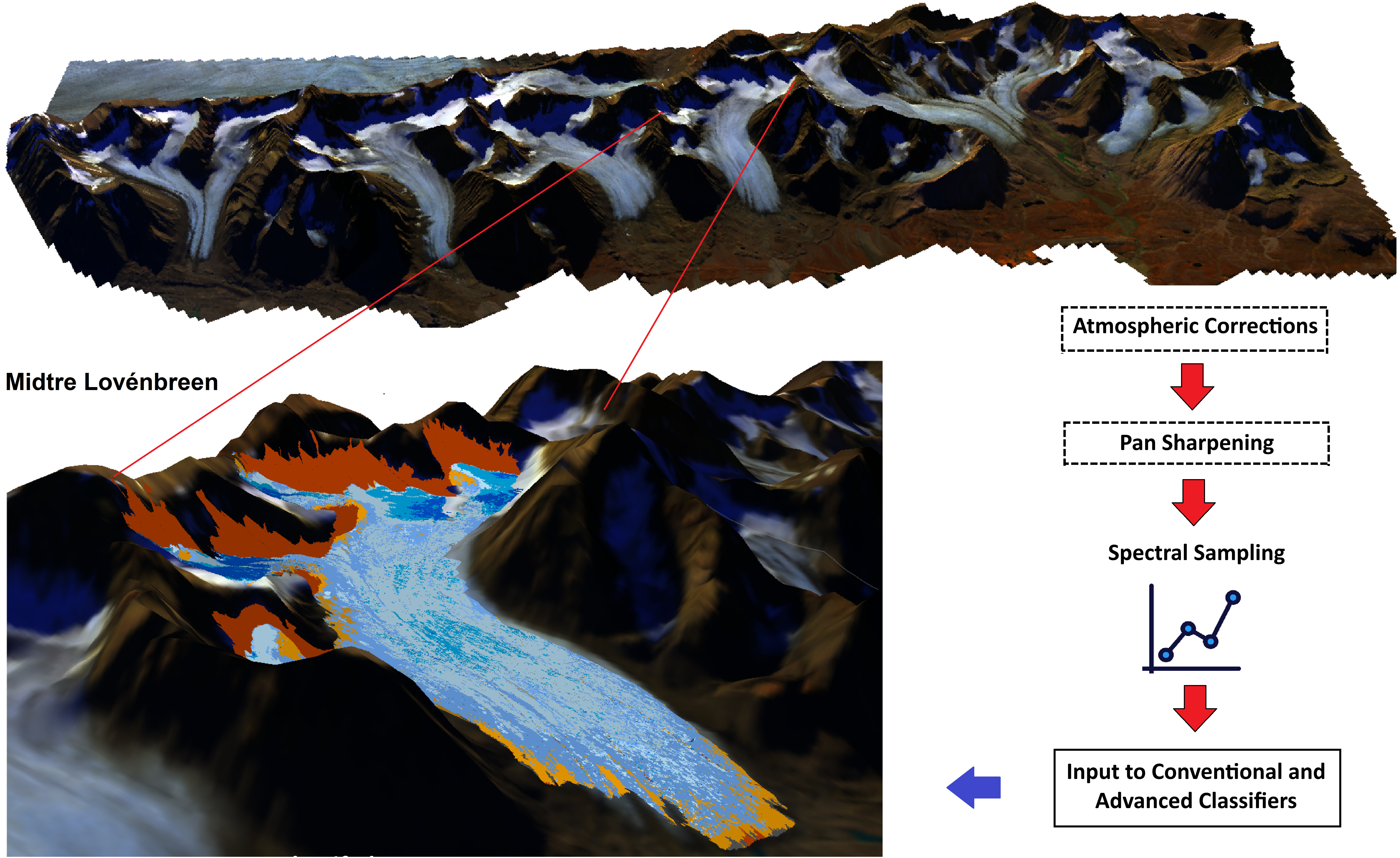
2.1.1. Site A: Ny-Ålesund, Svalbard

The Nordic archipelago of Svalbard is a pristine mass of glacial landscapes in the Arctic Ocean between 75° and 82°N [69]. An interplay of different oceanic currents and variation in atmospheric circulation causes this landscape to experience climates ranging from continental to coastal, with further fluctuations between winter, spring, and summer months [70]. Currently, this system is one of the most rapidly warming areas on the planet. The rate of its increase in temperature is reportedly double the global average [71]. The direct effect of this warming is visible on its glaciers in the form of glacier thinning [72], recession of perennial snow cover to higher elevations [73], and near-surface densification of the accumulation zone [74]. Due to the aforementioned factors, the entire region is of international scientific significance. The research base at Ny-Ålesund is an ode to this significance, and is the primary hub for scientific endeavors in western Svalbard. The glaciers near Ny-Ålesund are polythermal in nature [75,76]. The glaciers selected for this study included Vestre Brøggerbreen (VB), Austre Lovénbreen (AL), Austre Brøggerbreen (AB), Midtre Lovénbreen (ML), Edithbreen (EB), Botnfjellbreen (BB), Pedersbreen (PB), and Uvérsbreen (UB) (Figure 1). ML and AB are perhaps the most well documented of the selected glaciers. One of the earliest accounts of ML is a photographed documentation by Hamberg [77]. The Norwegian Polar Institute set up regular monitoring of mass balance for glaciers AB and ML in 1966 and 1967, respectively [69,78]. Furthermore, glacier surface facies were mapped on ML prior to this attempt by Pope and Rees [10,16], thereby presenting a working knowledge basis for direct comparison. Luis and Singh [60] also attempted to identify facies on the nearby Edithbreen glacier.

2.1.2. Site B: Chandra–Bhaga Basin, Himalaya

Known as the “Water Tower of Asia” [79], the Himalayas are a mountain chain of extreme cultural, sociological, economic, geopolitical, and strategic significance. Their cumulative scientific importance is, hence, phenomenal. In response to changing climates, the Himalayan cryosphere is receding, and has been observed to be losing frozen mass at an alarming rate [80]. The Indian Himalayas are well documented through both Survey of India (SOI) topographic maps and remote observations [81]. The hostile mountain terrain, vast landscape, and harsh weather conditions are often incumbent to field investigations, which result in certain pockets of glacier basins being selected for continuous monitoring. The Chandra–Bhaga basin is one such region. This basin is in the Lahaul and Spiti district of Himachal Pradesh, India. It lies within the monsoon–arid transition zone, and was therefore an optimal choice for studying glacial climatic response [82]. Himansh, the Indian Himalayan research base, is situated here at an altitude of 4080 m above mean sea level [17]. The glaciers selected were Samudra Tapu (ST), CB1, CB2, CB3, CB4, CB5, and CB6 (Figure 1). Samudra Tapu in the Chandra–Bhaga basin is analogous to Midtre Lovénbreen in Ny-Ålesund, as both are well monitored and provided established results for comparison. Alphanumeric identifiers were assigned to glaciers for which, to the best of our knowledge, no name has ever been assigned. Some of the studies over ST consisted of snow cover change analysis over four decades [83], snowline altitude changes for three decades [79], glacier facies mapping using VHR data [17,84], and debris cover variation analysis [85,86].
Table 1 documents all the selected glaciers from Ny-Ålesund and the Chandra–Bhaga basin, their respective areal extents, and their Global Land Ice Measurements from Space (GLIMS) reference ID [87].

2.2. Geospatial Data

The core datasets of this study were LV2A-processed images obtained from Digital Globe, Inc., Westminster, CO, USA [88]. The Himalayan image was acquired on 16 October 2014 (imagery © 2014 Maxar). In the Chandra–Bhaga basin, that period is just after the ablation season and the early onset of winter. It had a multispectral (MSL) resolution of 2 m and a panchromatic (PAN) resolution of 0.5 m. The Svalbard image was acquired on 10 August 2016 (imagery © 2016 Maxar). In Ny-Ålesund, this is right at the end of the ablation season. This arctic product had an at-nadir spatial resolution of 1.24 m, whereas the SWIR bands and PAN band had resolutions of 3.7 m and 0.31 m, respectively. The datasets had a radiometric resolution of 16 bits per pixel. The spectral resolution of WV-2 consisted of the bands PAN (0.45–0.80 µm), coastal (0.40–0.45 µm), blue (0.45–0.51 µm), green (0.51–0.58 µm), yellow (0.585–0.625 µm), red (0.63–0.69 µm), red edge (0.705–0.745 µm), near-infrared 1 (NIR1) (0.770–0.895 µm), and near-infrared 2 (NIR2) (0.86–1.04 µm). The projection and datum of the Svalbard image were done with WGS 1984 UTM Zone 33N, whereas the Himalayan image was projected with WGS 1984 UTM Zone 43N.
Pansharpened scenes were draped on 30 m Advanced Spaceborne Thermal Emission and Reflection Radiometer (ASTER) and Global Digital Elevation Model (GDEM) v2 [89] for the Chandra–Bhaga basin, and 5 m Arctic DEM [90,91] for Ny-Ålesund. The resultant 3D view of the study areas presented reliable surfaces for digitization of glacial boundaries [9,17].

3. Data Processing Methodology

3.1. Experimental Setup

The review of literature suggested utilizing the VNIR range of VHR optical data to exploit sensor-specific methods of mapping facies, specifically band ratioing. Comparison of outputs between ratios is beneficial to outlining the role of each band in mapping procedures. Based on the findings by Paul et al. [11] and Pope and Rees [16], it was observed that higher spatial and spectral differences in VHR data could improve the mapping outputs of glacier facies and deliver potentially superior results. Conventional and advanced supervised pixel-based classifiers (PBC) methods have also been shown to deliver good results in glaciological applications [17,59]. Finally, assessment of the effects of atmospheric corrections and pansharpening on the spatial and spectral differences induced by VNIR VHR data would thoroughly define an ideal processing protocol, as well as mapping mechanism. Figure 2 outlines the broad experimental setup of the current study.
This study aimed to map facies for selected glaciers in Ny-Ålesund, Svalbard; and the Chandra–Bhaga basin, Indian Himalayas, using VNIR VHR WV-2 data. Three different atmospheric corrections; viz., DOS, FLAASH, and QUAC, were used to derive reflectance, followed by pansharpening using GS and HCS. Glacial extents were defined by delineating 3D raised images over ASTER GDEM v2 and Arctic DEM, respectively. The subsets were then classified using conventional and advanced PBC methods, and the results were assessed using error matrices and qualitative assessment against published literature. Thus, the study used three atmospheric corrections, two pansharpening methods, and a host of classification algorithms to test the effects of pansharpening, atmospheric corrections, and classification algorithms on mapping glacier surface facies. Henceforth in the manuscript, processing “levels” of datasets will be referred to as processing schemes to describe the stage of processing. Table 2 displays each processing scheme and its associated nomenclature in the study. This nomenclature will be used to refer to the datasets, the classification, and respective workflows.

3.2. Image Processing

3.2.1. Radiometric Calibration and Atmospheric Correction

Conversion of DN to reflectance is a dual-step procedure, which involves: (a) converting digital number/brightness values to at-sensor spectral radiance; and (b) retrieving apparent surface spectral reflectance from at-sensor spectral radiance through atmospheric correction. The first step was carried out using the radiometric calibration module in Environment for Visualizing Images (ENVI) 5.3. This study tested three atmospheric correction models; each procedure is described as follows.
The FLAASH correction is a two-step process that requires: (1) retrieval of atmospheric parameters such as aerosol description and the water column amount; and (2) using the model atmosphere and aerosol description to convert radiance to reflectance using the radiative transfer code [92]. The atmosphere model [93] and aerosol model [94] were defined using the guidelines prescribed by Abreu and Anderson [95]. Other parameters such as initial visibility and GMT were user-defined using the image metadata. Factors including pixel size, aerosol height, CO2 mixing ratio, water column multiplier, zenith angle, sensor altitude, and scene center location were computed automatically upon definition of the sensor type. Table 3 highlights the parameters used for the images of each study area.
Unlike the FLAASH model, the QUAC correction is relatively straightforward. Described in [51] as an in-scene approach, it relies primarily on central wavelengths and the first step of sensor calibration. Due to this, the procedure directly involves input of the image into the QUAC module, which delivers the output scaled to a reflectance factor of 10,000 [92]. A simple band math correction brings the reflectance values into the range of 0–1. Like QUAC, the DOS correction is also an image-based corrective procedure. DOS is based on the principle that contributions of atmospheric scattering cause upwelling of the path radiance in dark pixels of an image in the concerned spectral [96]. Zhang et al. [97] outlined the DOS equation while stating that a single dark value was used to determine path radiance. For analyzing spectral signatures and subsequent classification, the imagery must be converted to reflectance. Therefore, following Rumora et al. [98], TOA reflectance was used an input to the DOS correction. Moreover, DOS correction in ENVI can incorporate user-defined dark pixel values. The procedure simply involves an operator-assisted identification of a few dark pixels and calculation of the average reflectance of each of the dark pixels. These average values can then be manually added into the DOS module window in ENVI 5.3 for each spectral band. Table 4 displays the average user-defined dark pixel reflectance values.

3.2.2. Pansharpening and Digitization

Pansharpening was performed in this study to test the differences between the GS, which is the most purported algorithm for retaining spectral information [40], and the HCS, which was designed for WV-2 imagery [42] against non-pansharpened imagery. GS estimates the panchromatic data based on the spectral response function of a given sensor [99]. The procedure requires direct input of the images into the GS module in ENVI. HCS sharpens MS imagery by replacing the intensity component of MS data in the hyperspherical color space with the intensity-matched form of the PAN band [44]. The procedure requires input of the PAN and MS images into the HCS fusion module in ERDAS IMAGINE.
Pandey and Venkatraman [79] experienced difficulties while manually digitizing ice divides and the glacier terminus. Bhardwaj et al. [9] resolved this issue by generating a 3D perspective of the area to observe and delineate the glacial boundaries. Jawak et al. [17] followed a similar approach, and highlighted the efficiency by which ice divides can be observed using the same method. Therefore, the current study followed suit by draping the GS-pansharpened imagery over the Arctic DEM for Ny-Ålesund and over the ASTER GDEM v2 for the Chandra–Bhaga basin. The glacial boundaries and ice divides were then digitized and extracted from the complete image using ArcGIS.

3.3. Glacier Facies Mapping Using Advanced Image Processing

Pixel-Based Classification

A wide variety of pixel-based algorithms can be employed for information extraction. Pope and Rees [10] used an unsupervised ISODATA algorithm to map facies. However, their base image was acquired using an Airborne Thematic Mapper (ATM). While this provided a good comparison against the Linear Combinations (LCs) of their study, it cannot be directly applied to satellite data. Supervised algorithms, on the other hand, have been used to map facies using satellite data [17,32,35,60,82] with good accuracies. Moreover, this study intended to improve upon comparisons between supervised classifiers [100] and test the effects of image-processing routines on the classification outputs. Such a test acts on the mathematical and computational differences between each classifier, a discussion that is beyond the scope of this paper. Nevertheless, as end users of classification algorithms, it was necessary to identify and evaluate their thematic performance. A comprehensive test of this scale would necessitate assessment of conventional and advanced pixel-based classifiers. ENVI offers both under its Terrain Categorization (TERCAT) and Target Detection (TD) workflows. Selected algorithms comprised Mahalanobis Distance (MHD), Maximum Likelihood (MXL), Minimum Distance (MD), Spectral Angle Mapper (SAM), Winner Takes All (WTA), Adaptive Coherence Estimator (ACE), Constrained Energy Minimization (CEM), Matched Filtering (MF), Mixture-Tuned Matched Filtering (MTMF), Mixture-Tuned Target-Constrained Interference-Minimized Filter (MTTCIMF), Orthogonal Space Projection (OSP), and Target-Constrained Interference-Minimized Filter (TCIMF). Table 5 describes each algorithm, the workflow under which they were available in ENVI, and reference studies in which the algorithms were used for information-extraction applications.
MHD, MXL, MD, and SAM are some of the most widely used and popular classifiers [133]. WTA is an ensemble of the majority classification from MHD, MXL, MD, and SAM. The CEM, MF, and OSP classifiers have been used for mapping glacier facies (Table 5). However, the other AC algorithms have been tested in applications requiring minute spectral differentiation (Table 5), and theoretically should be capable of discriminating between closely matching spectra of surface facies. Therefore, a comparative assessment of thematic classification among the popular and advanced algorithms using different processing schemes would lead to a greater understanding of their capabilities at identifying facies.
PBC is usually a two-step procedure requiring: (1) selection of training samples (regions of interest); and (2) application of supervised algorithms. Training samples were assigned based on visual and spectral analysis of the available facies. Polygonal regions of interest (ROIs) were outlined for each facies to accommodate their spectral variations (Supplementary Figure S1). Distribution of ROIs in percentage for the Chandra–Bhaga basin were as follows: snow was assigned 42.12%, glacier ice was assigned 20.82%, ice mixed debris was assigned 8.74%, and crevasses were assigned 9.10%; whereas shadowed area and debris were assigned ROIs containing 12.04% and 7.18%, respectively. For ROIs of the Ny-Ålesund glaciers, snow was distributed at 3.42%, streams and crevasses at 4.19%, shadowed snow at 22.36%, saturated snow at 11.57%, melting snow at 7.42%, melting glacier ice at 18.71%, and glacier ice at 20.23%; while dry snow and dirty ice were distributed at 3.34% and 8.76%, respectively. The MF, MTTCIMF, and MTMF algorithms required the imagery to undergo a minimum noise fraction (MNF) transformation prior to classification. Algorithms that did not require this transformation were processed directly after input of the image and ROIs into the respective workflows. Default parameters were retained in the workflows, and postclassification processing was avoided to negate unintentional analyst bias. Therefore, as performed by Jawak et al. [17], the stretch (square root) and rule thresholds (0.4) were common for each facies, for all classifiers, and for all the processing schemes.

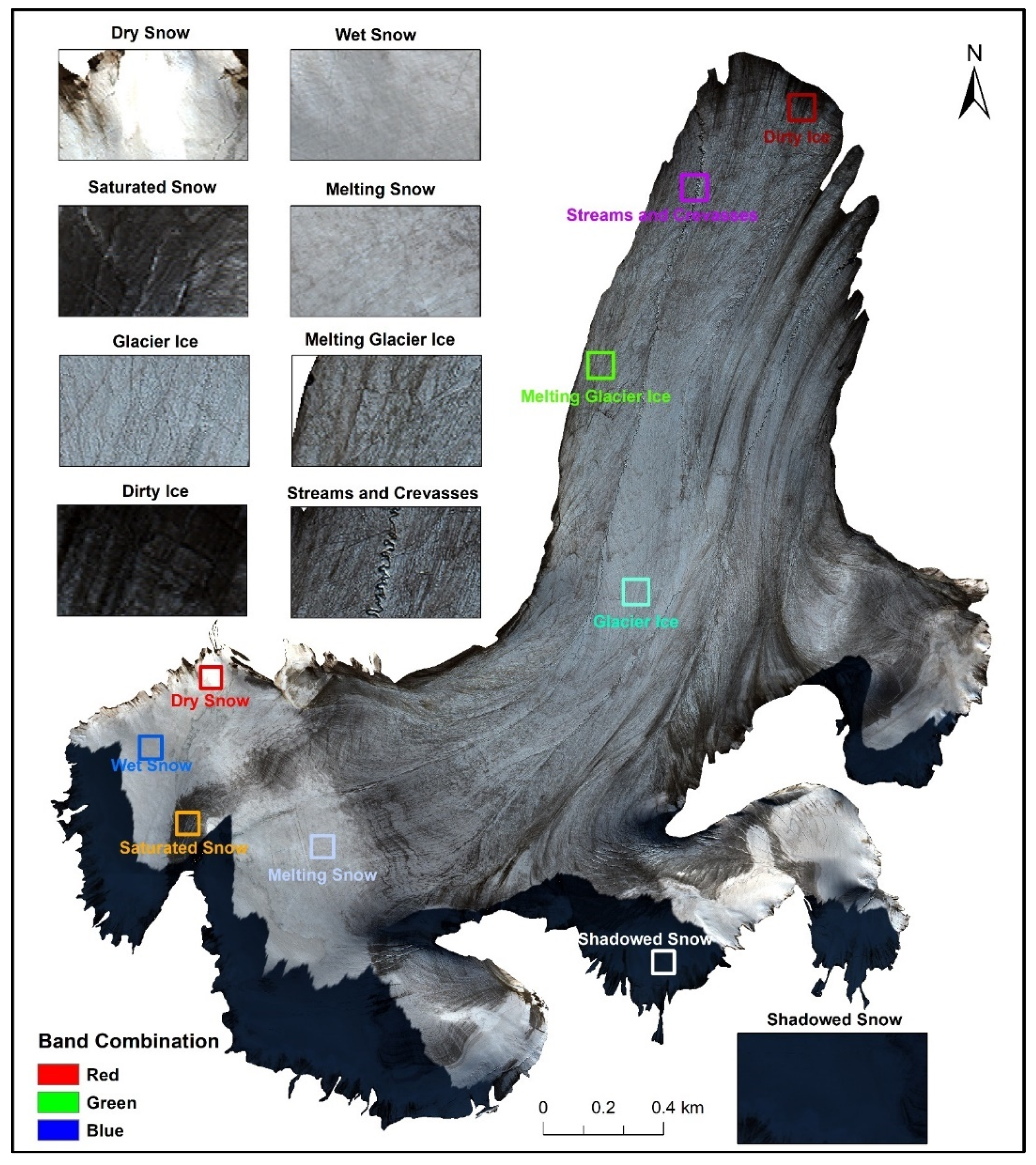
3.4. Identification of Surface Facies

In this study, glacier surface facies were identified in Ny-Ålesund and the Chandra–Bhaga basin using visual and spectral characteristics. Jawak et al. [17] described the visual identification of surface facies in the Chandra–Bhaga basin using the smoothness and higher elevation of snow, rougher and flow-induced striated texture of ice, disheveled structure of crevasses, and brightness variations between debris and ice mixed debris (IMD).
The same characterization was incorporated here to identify facies and derive spectral signatures for the Himalayan glaciers. A similar logic of surficial appearance, texture, and tonal variations, along with location on the glacier, was incorporated to identify surface facies on Ny-Ålesund glaciers. Figure 3 highlights the visual characteristics of observable surface facies on the ML glacier. The Chandra–Bhaga basin image was obtained at the start of early winter; hence, it showcased a large distribution of snow and glacier ice. However, the Ny-Ålesund image was obtained at the end of the ablation season, thereby showcasing the full range of surface facies. Facies identified on Ny-Ålesund glaciers consisted of dry snow, wet snow, melting snow, saturated snow, glacier ice, melting glacier ice, dirty ice, and streams and crevasses. Dry snow was characterized by its bright appearance at the highest elevation of the glacier. Wet snow appeared next, having a reduced brightness due to an increased moisture content than dry snow, but still maintaining an overall smoothness. Melting snow had more visible tonal roughness than wet snow, whereas saturated snow was much darker. This could be due to the high moisture and low integrity of the surface cover. Glacier ice was distinguishable through flow-induced striations and was distinct from melting glacier ice by its brighter appearance. Greater moisture and surface dust were the next possible reasons for its visual characteristic. Streams and crevasses were grouped together, as their individual characterization was difficult when much of the glacier’s surface appeared crevassed due to flowing supraglacial stream channels. Dirty ice was the darkest ablation facies characterizable, and functionally comprised more dust and debris toward the end of the glacial tongue.
Multispectral mapping of any earth feature entails utilization of spectral characteristics of the target feature. This requires good operator/analyst knowledge when field data is not available for reference. In this study, the spatial characteristics of facies were instrumental in identifying target sites. However, it was the spectral signatures that ultimately determined the separability of surface facies. As accuracies of spectral signatures rely upon the image-processing schemes employed, the current study presents the derived reflectance of facies identified on Ny-Ålesund glaciers in Figure 4 and the reflectance of facies identified on the Chandra–Bhaga basin glaciers in Figure 5. A detailed discussion of the variations in spectral signatures using each processing scheme is provided in Section 4.1.

3.5. Thematic Accuracy Assessment

The acquired satellite data could not be corroborated with field data due to harsh field conditions in the season of acquisition in the Himalayas and logistical difficulties in transit to Svalbard. In order to overcome this, the study followed an equalized random-sampling approach to assign reference points for analysis [134]. This approach provided every thematic class with an equal number of reference points [135]. To accommodate spatially limited facies, every class was allotted 10 reference points. Thus, for Ny-Ålesund glaciers, it resulted in 90 points per glacier, resulting in 720 pixels in total. For the Chandra–Bhaga basin glaciers, it resulted in 420 pixels in total. Bias was avoided in determining reference pixels by developing them independent of each other and by using polygons for ROIs and points for reference data. Confusion matrices were generated to calculate measures such as precision, recall, F1 score, overall accuracy (OA), error rate (ER), and specificity. Maxwell and Warner [136] described each measure, and Supplementary Table S1 displays the equations used to calculate precision, recall, F1 score, specificity and OA. ER was defined simply as “1-OA”. The measures were computed for every facies over each glacier individually, and were sequentially averaged to obtain mean values for each measure.

4. Results and Discussion

4.1. Spectral Signatures

The spectral characteristics of glacier surface facies are an account of snow ageing, metamorphosis, dust and debris entrainment, atmospheric depositions and a historical archive of glacial health, if monitored over long temporal scales. A change in reflectance characteristics is not only significant for ascertaining the state of changing snow and ice, but also for the understanding of possible causes for the visible change. This places a large importance on the selection of atmospheric-correction algorithms for deriving reflectance, and subsequently, spectral signatures. Figure 4 highlights the changes in spectral reflectance for each facies from Ny-Ålesund for each processing scheme. Figure 5 displays the variations induced by the respective processing schemes in derived spectral reflectance for facies observed in the Chandra–Bhaga basin. Both figures display the average reflectance for each facies. The reader is referred to Jawak et al. [17] for a detailed analysis of the spectral signature of facies derived in the Chandra–Bhaga basin. As the FLAASH atmospheric correction previously delivered the reflectance spectra most comparable with previous works, the characterizing of facies in the present analysis of Ny-Ålesund glaciers was initially performed using reflectance delivered by the same. Cassachia et al. [137] defined dry snow as not being subjected to melting or infiltration of water, and in principle it should be limited to the highest elevations on the glacier. No presence of water implied that facies with the highest reflectance would correspond to dry snow. Warren [138] described snow reflectance as being influenced by grain size, thickness of snow pack, mixing of dust and impurities, and moisture/liquid water content. Facies having a lower reflectance in the NIR region, but higher than other facies, would directly correspond to snow having greater moisture, and little to no surface impurities. Wet snow in this study was characterized by similar features. Wet snow and melting snow had a higher reflectance than fully saturated snow. The FLAASH-derived spectral signature of saturated snow closely matched that observed by Hinkler et al. [139]. The reflectance curves of dirty ice and glacier ice observed here were similar in trend to the curves depicted by Gao and Liu [140], who adapted their method from Zeng et al. [141]. Melting glacier ice identified here corresponded to that observed by Pope and Rees [10]. Table 6 displays bandwise-calculated variances for atmospheric corrections, GS pansharpening, and HCS pansharpening, according to maximum and minimum variance for each facies, averaged across all glaciers from the two test sites. Among the Chandra–Bhaga basin glaciers, snow class showed the maximum variation (0.31) among the atmospheric correction methods, whereas debris class showed the minimum variation (0.01). Snow and debris classes showed the same trend among the GS-sharpening (max: 0.29, min: 0.01) and HCS-sharpening processing schemes (max: 0.31, min: 0.01). For the Ny-Ålesund glaciers, dry snow exhibited a maximum variation of 0.20, while dirty ice showed a minimum variation of 0.00, for the atmospheric correction methods. For the GS sharpening schemes, dirty ice showed the maximum variation at 0.6; whereas the lowest variation was shown by shadowed snow at 0.01. The HCS sharpening schemes showed a maximum variation of 0.20 for dry snow, and a common minimum of 0.00 for shadowed snow and dirty ice. Section 4.3 discusses these variations in further detail.

4.2. Quantitative Analysis of Mapped Facies

This section analyzes classification results generated from the AC and CC workflows as an average of all the processing schemes for areal distribution and accuracy. Results are displayed for the glacier subsets ML and ST, and are presented according to the outputs for each facies.

4.2.1. Area per Facies Produced by Each Classifier

Areas of facies for Ny-Ålesund (reference glacier ML) and for the Chandra–Bhaga basin (reference glacier ST) are provided in Table 7 and Table 8.
Among the AC classifiers, the largest unclassified area for ML was given by TCIMF (0.20 km2), whereas OSP and MF produced the lowest unclassified area of 0.03 km2. Dry snow was given the largest distribution by ACE (0.64 km2) and the lowest by MTTCIMF (0.14 km2). Wet snow was classified with maximum areal distribution by MTMF (0.68 km2). The lowest distribution was reported by CEM at 0.45 km2. Melting snow achieved maximum distribution through MTTCIMF and the lowest through ACE at 0.63 km2 and 0.31 km2, respectively. MTTCIMF classified saturated snow at 0.72 km2, whereas the lowest distribution of saturated snow was produced by MTMF at 0.46 km2. The largest distribution of shadowed snow was provided by MTMF at 0.81 km2, and the lowest was delivered by OSP at 0.50 km2. Glacier ice was assigned the largest area by OSP at 0.60 km2, and the lowest at 0.29 km2 by TCIMF. Melting glacier ice was given the largest area at 0.74 km2 by ACE, and the lowest at 0.58 km2 by CEM. Dirty ice was distributed by CEM to a maximum of 0.93 km2, while ACE provided it with the lowest at 0.57 km2. Streams and crevasses were assigned the most area by MTTCIMF (0.42 km2), and the lowest by MF at 0.23 km2. Among the CC classifiers for ML, WTA assigned 0.02 km2 to unclassified, 0.16 km2 to dry snow, 0.38 km2 to wet snow, and 0.65 km2 to melting snow. Saturated snow, shadowed snow, and glacier ice were assigned 0.66 km2, 0.79 km2, and 0.54 km2, respectively. Melting glacier ice, dirty ice, and streams and crevasses were assigned 0.76 km2, 0.48 km2, and 0.32 km2, respectively.
For the reference glacier ST, among the AC methods, unclassified areas were provided with the largest area (0.81 km2) by MTTCIMF and MF, and with the least area by OSP (0.35 km2). Crevasses were mapped with the largest areal distribution at 6.22 km2 by MTTCIMF and the lowest at 4.05 km2 by MTMF. Glacier ice was mapped at 22.68 km2 by MTMF and 15.61 km2 by CEM. IMD was given the largest area at 10.44 by OSP km2, and the lowest at 4.04 km2 by ACE. Shadowed snow was mapped at 8.44 km2 by ACE and 1.93 km2 by MF. Debris cover was given a maximum areal extent of 10.77 km2 by MTTCIMF, and a lowest at 6.23 km2 by CEM. Snow was given the largest area at 34.17 km2 by CEM, and the lowest area for snow was given by OSP at 25.59 km2. Among the CC classifiers for ST, WTA classified 37.26 km2 as snow, 2.37 km2 as debris, and 1.65 km2 as shadowed snow. IMD, glacier ice, and crevasses were distributed as 1.84 km2, 27.71 km2 and 4.81 km2, respectively. Unclassified area totaled 0.37 km2. WTA was the ensemble of all CC methods, therefore its areal distribution was cumulatively affected by the area provided for each facies by the preceding CC algorithms.

4.2.2. Accuracy Achieved by Each Classifier

All measures of accuracy for all the classifiers are provided in Supplementary Sheet S1. This section aims to analyze the classification results of the AC and CC classifiers, and presents the F1 score as the harmonic mean of precision and recall [136] for each classifier as an average of all the processing schemes. This was to utilize the F1 score as a measure of reliability of the classification, independent of processing schemes.
(a)
F1 score for classification in Ny-Ålesund
Among the AC classifiers, dry snow was classified with a F1 score of 0.80 by ACE and 0.19 by TCIMF, whereas CEM, MF, MTMF, MTTCIMF, and OSP yielded an F1 score of 0.00. Similarly, wet snow was classified with an F1 score of 0.11 by ACE, 0.07 by TCIMF, and 0.00 by the other AC classifiers. Melting snow was classified with an F1 score of 0.36 by ACE, 0.18 by MTMF, 0.05 by OSP, and 0.04 by TCIMF. Saturated snow was mapped by ACE with an F1 score of 0.40, 0.22 by CEM and MF, 0.19 by OSP, 0.17 by MTMF, 0.04 by TCIMF, and 0.00 by TCIMF. Shadowed snow was classified with an F1 score of 0.00 by MTTCIMF, 0.10 by TCIMF, 0.20 by OSP, 0.21 by MTMF, 0.80 by ACE, and 0.33 by both CEM and MF. OSP and MTTCIMF classified glacier ice with an F1 score of 0.00, while TCIMF resulted in 0.04, MTMF in 0.15, and ACE in 0.51. CEM and MF each resulted in an F1 score of 0.21. Melting glacier ice was classified with an F1 score of 0.37 by CEM and MF, 0.11 by MTMF and OSP, 0.29 by ACE, and 0.04 by TCIMF. Dirty ice was mapped with a F1 score of 0.00 by MTTCIMF. CEM and MF yielded scores of 0.46 each, while ACE scored the highest with 0.54. OSP, TCIMF, and MTMF yielded scores of 0.13, 0.18, and 0.05, respectively. Streams and crevasses each were mapped by CEM and MF with an F1 score of 0.32, whereas ACE delivered an F1 score of 0.51, and MTMF delivered 0.07; MTTCIMF, OSP, and TCIMF delivered 0.00. Among the CC classifiers, MXL delivered a full F1 score of 1.00 for dry snow and shadowed snow, followed by 0.81 for streams and crevasses. Glacier ice and dirty ice were mapped by MXL with F1 scores of 0.74 and 0.73, respectively. Wet snow and melting snow were mapped with F1 scores of 0.69 and 0.68, respectively, by MXL. Melting glacier ice and saturated snow were classified by MXL with output F1 scores of 0.57 and 0.53, respectively. MHD classified both dry snow and shadowed snow with an F1 score of 0.93, while glacier ice achieved 0.72, dirty ice yielded 0.67, streams and crevasses resulted in 0.58, and saturated snow and melting snow achieved 0.47 and 0.45, respectively. Melting glacier ice and wet snow were classified with F1 scores of 0.39 and 0.33, respectively. MD classified dry snow with an F1 score of 0.96, while shadowed snow was classified with a score of 0.64. Melting snow and glacier ice scored 0.48 each. Dirty ice was mapped with a result of 0.47; glacier ice, saturated snow, and wet snow were classified with scores of 0.35, 0.30, and 0.24, respectively. Streams and crevasses were given a classified F1 score of 0.13. SAM classified shadowed snow with an F1 score of 0.83 and dry snow with an F1 score of 0.75, whereas melting glacier ice achieved 0.54, followed by wet snow at 0.48 and melting snow at 0.44. Glacier ice and saturated snow were classified with scores of 0.33 and 0.29, respectively; followed by dirty ice and streams and crevasses at 0.22 and 0.17, respectively. The WTA classifier achieved an F1 score of 0.95 for dry snow and shadowed snow, followed by streams and crevasses and glacier ice at 0.78 and 0.75, respectively. Dirty ice and saturated snow were classified with scores of 0.69 and 0.53, respectively. Melting snow and melting glacier ice achieved scores of 0.50 and 0.47 each. Lastly, wet snow was classified with a score of 0.38. Reliability orders for each facies are presented according to the classifiers. The reliability order for dry snow was: MXL > MD > WTA > MHD > ACE > SAM > TCIMF > CEM = MF = MTMF = MTTCIMF = OSP. The reliability for wet snow was: MXL > SAM > WTA > MHD > MD > ACE > TCIMF > CEM = MF = MTMF = MTTCIMF = OSP. The reliability of melting snow was: MXL > WTA > MD > MHD > SAM > ACE > MTMF > OSP > TCIMF > CEM = MF = MTTCIMF. Saturated snow presented the following reliability order: MXL = WTA > MHD > ACE > MD > SAM > CEM = MF > OSP > MTMF > TCIMF > MTMF. The reliability for shadowed snow was: MXL > WTA > MHD > SAM > ACE > MD > CEM = MF > OSP > MTMF > TCIMF > MTTCIMF. Glacier ice presented the following reliability order: WTA > MXL > MHD > ACE > MD > SAM > CEM = MF > MTMF > TCIMF > MTTCIMF = OSP. The reliability order for melting glacier ice was: MXL > SAM > MD > WTA > MHD > CEM = MF > ACE > MTMF = OSP > TCIMF > MTTCIMF. Dirty ice presented the following reliability order: MXL > WTA > MHD > ACE > MD > CEM = MF > SAM > TCIMF > OSP > MTMF > MTTCIMF. The reliability order for streams and crevasses was: MXL > WTA > MHD > ACE > CEM = MF > SAM > MD > MTMF > MTTCIMF = OSP = TCIMF.
(b)
F1 score for classification in the Chandra–Bhaga basin
Among the AC classifiers, crevasses were mapped with an F1 score of 0.69 by ACE, 0.53 for both CEM and MF, 0.17 for both MTMF and OSP, 0.21 for TCIMF, and 0.07 for MTTCIMF. Glacier ice was classified by CEM and MF with a common F1 score of 0.83, ACE delivered a score of 0.77, and MTMF scored 0.32. OSP and TCIMF delivered F1 scores of 0.21 each, whereas the lowest score was delivered by MTTCIMF (0.00). IMD was classified by ACE with an F1 score of 0.40. CEM and MF resulted in scores of 0.30 each. TCIMF resulted in a score of 0.21, whereas OSP produced a score of 0.19. MTMF delivered a score of 0.10, and MTTCIMF produced a score of 0.02. Shadowed snow was mapped by ACE with a score of 0.79, and TCIMF produced a score of 0.39. CEM, OSP, and MF delivered F1 scores of 0.34 each. MTMF and MTTCIMF delivered F1 scores of 0.33 and 0.00, respectively. Debris was mapped with a common F1 score of 0.23 for CEM, MF, and TCIMF. OSP and ACE provided scores of 0.22 and 0.16 each. MTMF and MTTCIMF resulted in scores of 0.07 and 0.00, respectively. ACE, CEM, and MF produced a common F1 score of 0.67 for snow, followed by MTMF with a score of 0.26. OSP and TCIMF mapped snow with a score of 0.23, whereas MTTCIMF delivered 0.00. Among the CC classifiers, MXL mapped crevasses with an F1 score of 0.80, MHD delivered a score of 0.79, whereas MD and SAM delivered scores of 0.67 and 0.28, respectively. Glacier ice was mapped with the highest F1 score of 0.96 by MD, followed by MXL with a score of 0.92. SAM and MHD were mapped with scores of 0.87 and 0.84, respectively. IMD was given the highest F1 score of 0.55, whereas SAM resulted in the lowest score of 0.00. MXL and MHD mapped IMD with scores of 0.47 and 0.41 each. Shadowed snow was classified with high scores of 0.93 and 0.90 by MHD and MXL, respectively; whereas MD and SAM were mapped with scores of 0.20 and 0.17, respectively. Debris was classified by MD with a score of 0.62. SAM and MHD delivered scores of 0.27 and 0.25, respectively; while MXL resulted in a score of 0.47. MD mapped snow with a high F1 score of 0.98, followed by MXL with a score of 0.97, and MHD at 0.95. SAM delivered a score of 0.77. WTA classified snow with an F1 score of 0.96, followed by shadowed snow with an F1 score of 0.95. Crevasses were subsequently mapped with a score of 0.89, followed by glacier ice at 0.88. IMD and debris were mapped with scores of 0.44 and 0.61 each. The order for reliable classification of crevasses was: WTA > MXL > MHD > ACE > MD > CEM = MF > SAM > TCIMF > MTMF = OSP > MTTCIMF. The reliability order for glacier ice was: MD > MXL > WTA > SAM > MHD > CEM = MF > ACE > MTMF > OSP = TCIMF > MTTCIMF. Ice mixed debris presented the following reliability order: MD > MXL > WTA > MHD > ACE > CEM = MF > TCIMF > OSP > MTMF > MTTCIMF > SAM. The reliability order for shadowed snow was: WTA > MXL > MHD > ACE > TCIMF > CEM = MF = OSP > MTMF > MD > SAM > MTTCIMF. Debris presented the following reliability order: MD > WTA > MXL > SAM > MHD > CEM = MF = TCIMF > OSP > ACE > MTMF > MTTCIMF. The reliability order for snow was: MD > MXL > WTA > MHD > SAM > ACE = CEM = MF > MTMF > OSP = TCIMF > MTTCIMF.
Table 9 gives an overall representation of classifier performance averaged over all the processing schemes. Apart from the ACE classifier, all other classifiers showed a greater error rate while classifying facies in Ny-Ålesund in comparison to the Chandra–Bhaga basin. The difference between them, however, was 0.01. The best-performing classifier was the MXL, while the worst was the MTTCIMF. The order of overall classifier performance was thus: MXL > WTA > MHD > ACE > MD > CEM = MF > SAM > MTMF = TCIMF > OSP > MTTCIMF.

4.2.3. Comparison between Atmospheric Correction Methods

Figure 6 displays the overall accuracy (OA) achieved by each of the classification algorithms across the atmospheric corrections. An analysis of the trends of the OA revealed a similar trend for all three atmospheric corrections. Averages and variances were calculated for both study areas for DOS, FLAASH, and QUAC. Visual analysis of Figure 6 depicts FLAASH as having the least total variance, with DOS and QUAC showing consistent variances. MXL and WTA achieved the highest OA.
The DOS_MXL classification showed no variance across both study areas, FLAASH_MXL classification achieved 0.01 variance, and the QUAC_MXL classification achieved a variance of 0.03. WTA classification varied by 0.05, 0.03, and 0.06 for DOS_WTA, FLAASH_WTA, and QUAC_WTA, respectively. DOS_MHD classification resulted in a variance of 0.07, FLAASH_MHD resulted in 0.03, and QUAC_MHD resulted in 0.04. DOS_MD resulted in a variation of 0.14, FLAASH_MD delivered a variance of 0.15, and QUAC_MD resulted in 0.04. DOS_ACE produced a variance of 0.06, FLAASH_ACE resulted in 0.04, and FLAASH_QUAC resulted in 0.10. DOS_SAM produced a classification variance of 0.03, FLAASH_SAM produced a variance of 0.03, and QUAC_SAM delivered 0.08. DOS_MTTCIMF delivered a variance of 0.02, FLAASH_MTTCIMF produced 0.01, and QUAC_MTTCIMF resulted in 0.16. DOS_MTMF classified with a resultant variance of 0.04, FLAASH_MTMF classified with a variance of 0.02, and QUAC_MTMF produced a variance of 0.07. DOS_CEM resulted in a variance of 0.24, FLAASH_CEM produced a variance of 0.38, and QUAC_CEM delivered 0.07. DOS_MF classified facies with a variance of 0.24, followed by FLAASH_MF at 0.01and QUAC_MF at 0.01. DOS_OSP classified facies with a variance of 0.03, FLAASH_OSP delivered 0.05, and QUAC_OSP produced 0.13. DOS_TCIMF produced a variance of 0.12, FLAASH_TCIMF delivered a variance of 0.00, and QUAC_TCIMF produced a variance of 0.09.
In summary, the classifier showing the most consistent performance across different atmospheric corrections and test sites was the MXL, followed by WTA. The atmospheric correction showing the least variation across the test sites was FLAASH. The highest OA was achieved by DOS_WTA (0.81), whereas the lowest was achieved by FLAASH_MTTCIMF (0.01). The order of reliability among the atmospheric corrections was: FLAASH > QUAC > DOS. This reliability was based upon the total variance in the OA across all the classifiers and both test sites. The reliability order of classifier performance averaged across both test sites for each atmospheric correction (based on OA) was: DOS_WTA > QUAC_MXL > DOS_MXL > FLAASH_MXL = FLAASH_WTA = QUAC_WTA > DOS_MHD > QUAC_MHD > DOS_MD = FLAASH_MD > DOS_ACE > FLAASH_MHD > QUAC_ACE > DOS_CEM = DOS_MF > QUAC_MD > FLAASH_ACE > DOS_SAM > FLAASH_CEM = FLAASH_MF = QUAC_SAM > QUAC_CEM > FLAASH_SAM > QUAC_MF > DOS_OSP = QUAC_TCIMF > DOS_MTMF = DOS_TCIMF > QUAC_OSP > FLAASH_MTMF > QUAC_MTTCIMF > FLAASH_OSP > FLAASH_TCIMF > QUAC_MTMF > DOS_MTTCIMF > FLAASH_MTTCIMF.

4.2.4. Effect of Pansharpening

Table 10 showcases the average error rate (both study areas) achieved by each classifier for each processing scheme when not pansharpened, GS sharpened, and HCS sharpened. The error rate was a suitable measure to highlight the changes in performance for each scheme. An initial analysis of Table 10 presented a general trend of decrease in classifier performance after pansharpening. GS_DOS_ACE showed an increase in error by 0.18 from DOS_ACE, whereas HCS_DOS_ACE increased by 0.28. The errors in GS_DOS_CEM and GS_DOS_MF increased by 0.32, whereas HCS_DOS_CEM increased by 0.33 and HCS_DOS_MF by 0.34. GS_DOS_MTMF showed a 0.00 increase in error, whereas HCS_DOS_MTMF increased by 0.06. MTTCIMF presents a case of decreasing error by 0.09 and 0.08 for the GS_DOS and HCS_DOS processing schemes, respectively. OSP classification had an increase in error of 0.17 for GS_DOS and 0.14 for HCS_DOS, respectively. TCIMF performance decreased by 0.12 for GS_DOS and 0.08 for HCS_DOS subsets.
MHD classification resulted in an increase in error of 0.36 for HCS_DOS and 0.12 for GS_DOS. MXL classification showed an increase in error of 0.27 for HCS_DOS and 0.03 for GS_DOS. MD performance showed an increase in error of 0.46 for HCS_DOS and 0.32 for GS_DOS. SAM showed an increase in the resultant error by 0.24 for HCS_DOS and 0.12 for GS_DOS.WTA classification increased in error by 0.41 for HCS_DOS and 0.15 for GS_DOS. For the FLAASH subsets, GS _FLAASH_ACE decreased in performance by 0.27, whereas the HCS_FLAASH_ACE classification showed an increase in performance by 0.05. HCS_FLAASH_CEM, HCS_FLAASH_MF, HCS_FLAASH_MTMF, HCS_FLAASH_MTTCIMF, HCS_FLAASH_OSP, and HCS_FLAASH_TCIMF showed an increase in classification performance by 0.01, 0.11, 0.12, 0.35, 0.16, and 0.34, respectively. GS_FLAASH_MTTCIMF, GS_FLAASH_OSP, and GS_FLAASH_TCIMF increased in performance by 0.10, 0.03, and 0.08, respectively. GS_FLAASH_CEM and GS_FLAASH_MF each showed a common decrease in performance by 0.16. GS_FLAASH_MTMF increased in error by 0.03. MHD classification decreased in performance by 0.35 and 0.08 for the GS_FLAASH and HCS_FLAASH subsets.
MXL classification increased in error by 0.50 and 0.47 for the HCS_FLAASH and GS_FLAASH subsets. GS_FLAASH_MD, GS_FLAASH_SAM, and GS_FLAASH_WTA increased in resultant error by 0.43, 0.23, and 0.48, respectively. HCS_FLAASH_MD, HCS_FLAASH_SAM, HCS_FLAASH_WTA decreased in performance by 0.44, 0.25, and 0.48, respectively. For the QUAC subsets, only GS_QUAC_MTTCIMF and HCS_QUAC_MTTCIMF showed a decrease in error by 0.12 and 0.41, respectively. GS_QUAC_ACE and HCS_QUAC_ACE showed an increase in error by 0.37 and 0.35, respectively. GS_QUAC_CEM and GS_QUAC_MF each showed a common increase in error of 0.20. Similarly, HCS_QUAC_CEM and HCS_QUAC_MF each resulted in a common increase in error of 0.17. GS_QUAC_MTMF and HCS_QUAC_MTMF resulted in an increase in classification error of 0.06 and 0.03, respectively. GS_QUAC_OSP and HCS_QUAC_OSP delivered an increase in error by 0.03 and 0.07 each. TCIMF classification of GS_QUAC and HCS_QUAC subsets resulted in an increase in classification error by 0.11 and 0.12, respectively. GS_QUAC_MHD and HCS_QUAC_MHD resulted in a decrease in performance by 0.47 and 0.18 each. MXL classification resulted in an increase in error by 0.56 for GS_QUAC and 0.24 for HCS_QUAC. GS_QUAC_MD and HCS_QUAC_MD increased in error by 0.27 and 0.17 each. SAM classification of the GS_QUAC and HCS_QUAC subsets delivered an increase in error by 0.21 and 0.11, respectively. GS_QUAC_WTA and HCS_QUAC_WTA resulted in an increase in classification error by 0.48 and 0.18, respectively. The average variance between DOS, GS_DOS, and HCS_DOS for each classifier produced the following order of increasing variability: MTMF < MTTCIMF < TCIMF < OSP < SAM < ACE = MXL < CEM < MF < SAM < WTA < MD. The average variance between FLAASH, GS_FLAASH, and HCS_FLAASH for each classifier resulted in the following variability order: MTMF < OSP < CEM < MF = SAM < ACE < MTTCIMF = TCIMF = MHD < MD < MXL < WTA. Variability between QUAC, GS_QUAC, and HCS_QUAC resulted in the following order: MTMF < OSP < TCIMF < CEM = MF = SAM < MD < ACE = MTTCIMF < MHD < WTA < MXL. While the MTMF produced the least varying classification between nonsharpened and pansharpened imagery, it possessed a high error for all the subsets of imagery tested in this study.
The cumulative average error rate for the pansharpened subsets revealed the following order of reliability: GS_DOS > HCS_FLAASH > HCS_QUAC > HCS_DOS > GS_FLAASH > GS_QUAC. Upon averaging the effects of atmospheric corrections, the HCS pansharpening was calculated to have a lower error rate (0.71) for all classification algorithms and all atmospheric corrections, when compared to the GS method (0.76). Figure 7, Figure 8 and Figure 9 display the thematic results of FLAASH_MXL and HCS_FLAASH_MXL.

4.3. Discussion

Atmospheric correction impacts the quality of observable and derivable spectral reflectance of desired targets. Section 1.4 highlights studies that compared atmospheric corrections and the complexity imbued in the selection process. The overarching consensus states that the choice of atmospheric correction is application-centric [61]. A careful assessment of the impact of atmospheric correction on the spectral signature of target facies in this study was presented in Section 4.1. Previously, the FLAASH correction was used to derive target spectral reflectance and then matched against existing literature for its validity [17]. In the current study, spectral signatures of facies derived from the FLAASH correction were used in the same capacity. The extracted signatures closely matched those observed in previous efforts (Section 4.1), based on the properties of reduced reflectance [62] and mixing of moisture, dust, impurities, and debris [138]. Subsequent extraction of spectral signatures of the same facies from subsets of each processing scheme revealed a variance between each scheme, and thereby, differences in the resultant classifications. The highest variances between DOS, FLAASH, and QUAC were most prominent in B1, B2, B7, and B8. This was potentially because B1 and B2 (Coastal and Blue) were used to provide atmospheric information [142,143], and were therefore affected the most by its effects, whereas B7 and B8 (NIR1 and NIR2) were predominantly affected by water absorption and dispersion of suspended particles [144]. Moreover, Chakouri et al. [57] suggested that the green-to-NIR spectrum is least affected by atmospheric scattering. Analysis of Figure 4 and Figure 5, as well as the maximum and minimum variations of spectra depicted in Table 6, highlighted that the reflectance spectra of facies derived from non-pansharpened imagery showed the least variations between B3 (Green) to B6 (Red Edge), and the most variations were observed at B1 (Coastal) for most of the facies. Reliability based on variance in OA across both study areas for all classifiers suggested that DOS was the worst performer. This was likely because DOS does not emulate atmospheric absorption, and produces a decrement of surface reflectance [145,146]. Moreover, as the minimum value of dark pixels was a combination of atmospheric effects, specular reflection, and skylight scattering from the entire image [147], the DOS configuration was too simplistic for separating overlapping spectral signatures from different classes. FLAASH was the most reliable atmospheric correction method, as the results of the classification from its subsets were the most consistent. This was believed to be due to close matching of FLAASH-derived reflectance with surface reflectance [148]. QUAC performed poorer than FLAASH in the current study, perhaps due to the nonexistence of a minimum of 10 distinct spectral classes [93,149]. Saini et al. [149] further went on to reiterate the realistic reflectance derived through FLAASH.
The literature review of pansharpening (Section 1.3) arrived at a task-specific conclusion, similar to that for atmospheric correction. A visual analysis of Figure 4 and Figure 5 highlighted the decrease in reflectance derived from pansharpened imagery. This implied an overall decrement in spectral signature characteristics. GS_DOS was found to have the most deterioration. Resultant spectra from HCS_DOS/FLAASH/QUAC were found to match closely with the nonsharpened DOS-, FLAASH-, and QUAC-derived spectra. This agreed with Rayegani et al. [47] and Padwick et al. [42]. Spectra of the Chandra–Bhaga basin snow class showed the highest variance (0.29) across GS_DOS, GS_FLAASH, and GS_QUAC. The highest variance across HCS_DOS, HCS_FLAASH, and HCS_QUAC was found for the spectra of the Chandra–Bhaga basin snow class (0.31). Moreover, variance in GS- and HCS-sharpened spectra for the Chandra–Bhaga basin facies was found to be higher than that of the Ny-Ålesund facies. Shadowed snow for both CB and Ny-Ålesund showed a much lower variance across the GS and HCS subsets than other facies. The spectral bands showing the most variance were B1, B2, B7, and B8. This was due to the obvious reason that atmospheric influences (for B1 and B2) were only reduced by appropriate correction algorithms, whereas the effects of moisture and particle mixing (B7 and B8) were target- and scene-specific. Ablation facies were characterized by increasing moisture, saturation, densification to ice and subsequent discharge of melt water. Therefore, the variations in B7 and B8 would most likely be persistent. Although HCS was more stable than GS across all its subsets according to its classification performance (Section 4.2.4), both resulted in a high error rate. One reason could be the compounding effect of the previous atmospheric corrections and subsequent variety of classification algorithms. Previous assertions of the utility of the GS method [38,39,40] did not hold true in the current study.

4.3.1. Classifiers and Surface Facies: Performance and Comparison

Jawak et al. [41] tested a variety of band ratios and classifiers, such as MTTCIMF, CEM, ACE, OSP, MTMF, MF, MXL, SVM, NNC, and SAM, to map Antarctic vegetation using WV-2 data. Their work showed the prowess of MTMF in mapping sparse vegetation patches. Moreover, the MXL was inefficient in their analysis by creating a maximum number of misclassified pixels. The current study, however, delivered the opposite results. Here, MXL and MD performed better than MTMF in an overall identification of facies. This contrasting result could be because the adjacent classes in their work; namely, landmass/rocks, water bodies, snow/ice on lakes and rocks, shadowed ice, shadowed landmass, melt water, and surface debris on snow/ice, were all highly distinctive in their spectral characteristics. In the case of the surface facies, distinct classes were based on reduction in reflectance properties induced by melt and mixing of particles. This was also noted by Jawak et al. [41] when shadowed ice and melt water on the surface of rocks caused significant misclassification in the AC methods. Kumar et al. [130] attempted to identify minerals at the subpixel level using MTTCIMF in mountainous areas of Rajasthan, India. Their results suggested that MTTCIMF performed poorly when there was high interclass similarity. Portions of the reflectance spectra of facies overlapped each other (Figure 5 and Figure 6), which could have caused poorer performance of MTTCIMF in facies applications. Curiously, MTTCIMF delivered higher accuracy for the GS and HCS subsets for all three atmospheric corrections. This could imply that pansharpening VHR imagery may improve target detection using MTTCIMF. An increase in accuracy was also observed for classification results of ACE, CEM, MF, MTMF, OSP, and TCIMF for the HCS_FLAASH subset. The greatest increase was for the HCS_FLAASH_MTTCIMF classification (0.35 increase, 35% improvement). Although the increase in performance did not improve the overall ranking of the classifiers to a large extent, it was an important factor to note, as an increase in the total number of pixels under the same polygonal unit of the concerned ROI could improve target detection when sharpened by HCS in this instance. Millan et al. [129] tested five AC methods (CEM, ACE, SAM, TCIMF, and MTMF) for estimating reflectance of targets of interest in mine-related flooded areas of Nord-Rhein Westphalia, Germany. They found variable performance of the classifiers for their targets, but recommended SAM, ACE, and MTMF, as targets were better classified using these. They inferred this, as the recommended classifiers showed low sensitivity to Bidirectional Reflectance Distribution Factor (BRDF) effects on target classes. In the current case, each glacier was carefully extracted from the complete imagery, nullifying any valley rock/nonglacier influence. Moreover, any BRDF influence observed over each glacier for the spectral bands would be uniform throughout the classification process, and should not have been a hindrance in the results of the current study [17]. Moreover, Millan et al. [129] also described the effectivity of specific classifiers for individual targets. Here, for the Ny-Ålesund facies, dry snow, wet snow, melting snow, shadowed snow, glacier ice, melting glacier ice, dirty ice, and streams and crevasses were best classified by MXL, whereas saturated snow was equally well classified by MXL and WTA. For the Chandra–Bhaga basin facies, crevasses and shadowed snow were best classified by WTA, whereas glacier ice, IMD, debris, and snow were best classified by MD. Jin et al. [150] tested MF, SAM, CEM, TCIMF, ACE, and OSP for target detection at subpixel and full-pixel scales over Cooke City, Montana, USA. Their findings suggested that classifiers based on matched filters (MF, CEM, MTMF, and TCIMF) had poor generalization, causing misclassification of pixels belonging to the same class but with slightly different spectral signatures. Poor performance of the MF-based classifiers in the current study supported the same inference. Furthermore, they found that the ACE classifier achieved better target visibility and classification than other AC methods. Here, ACE was the best performer of all the AC algorithms across all processing schemes, and therefore validated the same inference. Jawak and Luis [151] assessed the performance of SVM, MXL, NNC, SAM, and an ensemble WTA to map land cover in Larsemann Hills, Antarctica, using HCS-sharpened WV-2 imagery. They found that WTA performed best, while MXL performed worst. However, the accuracies of all methods were quite high. In the current study, MXL and WTA performed well across all processing schemes. The performance of SAM as shown by Jawak and Luis [151] depended upon the abundance and separability of spectral classes. A significant feature of their study was the nonoverlap of land cover classes, thereby resulting in high accuracy. The differences in facies, however, was not essentially a sharp contrast. The variations from accumulation to ablation can cause confusion if spectral signatures are not carefully considered. Moreover, SAM performed poorly here, leading to unclassified pixels, consequently causing unclassified pixels in the WTA classification. The default settings in ENVI were used to enable an unbiased analysis of classifier performance. This may have led to low representation of the maximum angle between the ROI and input pixel spectrum. Luis and Singh [60] attempted to map surface facies on the Edithbreen glacier in Ny-Ålesund, Svalbard, using VHR WV-3 and Landsat 8 OLI data. Their attempt focused on comparing pixel- and object-based methods. While the object-based methods thoroughly achieved the best results, the pixel-based results for MHD, MXL, and MD highlighted the robustness of MXL. However, MD performed poorly in their analysis, which countered the current findings; this could be possibly be due to the larger number of overlapping classes defined by Luis and Singh [60]. Albert [59] compared MXL, MD, parallelepiped (PP), SAM, ISODATA, linear unmixing, MTMF, a range of fuzzy classification methods, and band math indices/techniques to delineate ice cover around the tropical Quelccaya ice cap in Peru. The author used a DOS-corrected Landsat 5 TM image. The final processing steps involved conversion of radiance to reflectance units. However, in the current study, DN was first converted into radiance and then to TOA reflectance before performing user-defined DOS [98]. Albert [59] found SAM to be the most accurate of the supervised classifiers. This occurred due to testing of a variety of angular thresholds. The author noted that that the supervised classifiers performed well because snow and ice were one thematic class, rather than bifurcated into different snow and ice facies. This suggested that additional categories of closely matching spectra, but with distinct thematic features, may reduce the performance of many supervised classifiers. The results of the current study were consistent with this.
Pope and Rees [10] mapped glacier facies on the ML glacier using in situ spectral reflectance on field-observed surface classes of facies through ETM+ imagery classification. The authors used an unsupervised ISODATA algorithm and principle-component-derived linear combinations (LCs) to categorize surface classes. Several classes identified by the authors were based upon field assessment of grain size and visible/flowing water on the surface. The spectral reflectance signatures used for validation were collected a decade after the image acquisition. This was the opposite of the recent recommendation by Yousuf et al. [36], who suggested snow and ice validation data should be closely timed with the image capture. Due to nonavailability of field spectra, the current study relied on image and spectra interpretation and published literature for references and a comparison of spectral signatures (refer to Section 3.4 and Section 4.1, and [17]). The comparative pixel- and object-based characterization of glacier facies on the Edithbreen glacier by Luis and Singh [60] presented a curious case. Common classes between their work and the current study included dry and wet snow, melting ice, and shadow. Uncommon classes included percolation snow, dirty snow, debris, off-glacier, water stream, and crevasses. The separation of water stream and crevasses was avoided in the current study due to increased spectral confusion and probability of misclassification. Moreover, absence of in situ/reference spectra enhanced the chances of incorrect training of ROIs. Manual digitization of glacial boundaries negated the need for an off-glacier class. Furthermore, when comparing Landsat 8 (L8) and WV-3, their L8 classification showed a class called wet semisaturated snow. This class was identified by Pope and Rees [10] after in situ collection, and was separated from dry semisaturated ice by an increased amount of water on the surface. The quantity of water that marked the spectral contrast between wet snow and wet semisaturated snow was not easily identified with medium-resolution satellite data. Luis and Singh [60] touted the effectivity of the object-based indices; however, the thematic results showcased dirty “snow”, a snow surface facies class on the ablation area of the glacier, using WV-3, but then labeled the same as dirty ice in classification of L8 data. Nevertheless, their work provided an important reconnaissance for future effective mapping of surface facies in the region. The current study built upon their findings and objectively characterized facies using visual and spectral characteristics. Jawak et al. [17,33] mapped surface facies using a combination of pixel- and object-based classification techniques on FLAASH-corrected WV-2 data. Their goal was to effectively characterize facies for the Chandra–Bhaga basin region using VNIR VHR satellite data. The current study aimed to test the impacts of varying processing schemes on the overall classification of surface facies to determine the most efficient and accurate method for future mapping attempts. Testing of additional supervised classifiers such as TCIMF, MTTCIMF, MTMF, and ACE proved useful in highlighting the utility of matched filtering methods and the performance of ACE. Moreover, improvement in classification accuracy by MTTCIMF after pansharpening was an important clue to the potential implementation of the algorithm using in situ spectra and/or aerial imagery.

4.3.2. Computer Processing Time and Limitations

Successful data-driven remote sensing applications depend upon stable computational infrastructure. In the preceding sections, this study qualitatively and quantitatively assessed classified thematic results of different processing schemes. Therefore, it is now necessary to evaluate the computational requirements and loads of the individual schemes. To this end, the study considered factors such as data acquisitional challenges, system properties, time taken for processing, and storage space needed. The specifications of the primary system used to process data in this study (System A) consisted of 16 GB of RAM (DDR4), an SSD with 256 GB, an HDD with 1 TB, a ninth-generation Intel® Core™ i7-9750H (64-bit) processor, and a NVIDIA® GeForce® GTX 1650 (4GB) graphics card. In addition to this, an additional portable hard drive with more than 4 TB of storage was needed to store all the generated data. All files, beginning from calibration to classification, were saved in default ENVI formats to maintain uniformity. The HCS sharpening performed in ERDAS IMAGINE 15 necessitated input files in its default IMG imagine format. The HCS-sharpened files were then exported back into the default ENVI format (.dat) for further classification. This standardization of file formats was in line with the recommendations by Shcadt et al. [152] for big data management. Table 11 highlights the complete processing time and storage space needed, from calibration to classification, for each of the image-processing schemes for glaciers ML and ST. This presents an account of the practical limitations when processing data for such applications. In terms of the processing schemes, the GS and HCS products occupied the maximum disk space and processing time with no superior enhancements in accuracy. The Himalayan glacial subsets, being bigger in size, took the most space and time. AC classification of the Samudra Tapu GS_FLAASH subset had the largest file size (312 GB), and consequently took the most processing time (593 h) of all the subsets and processing schemes tested in the current study.
The smallest input file was the Midtre Lovénbreen DOS subset (0.44 GB). As an example of the comprehensive approach of the study, the total time for image calibration and classification of the glacial subsets of Samudra Tapu and Midtre Lovénbreen was 5247.05 h, with a combined disk size of 3909.80 GB. The CC methods, being lesser in number, consequently occupied less disk space. Considering the accuracies delivered by AC and CC algorithms (Section 4.2.2), and the respective times for processing and storage space (Table 11), it was evident that the CC methods were much more efficient.

4.3.3. Inherent Challenges and Limitations

In the quest for assessing image-processing impacts on mapping glacier facies, the current study encountered and attempted to resolve several computational challenges, as described in the sections above. However, some challenges for mapping facies and supraglacial terrain were inherent to this application itself. Factors such as cloud cover, seasonal snow, precipitation, and crevassed surfaces pose difficulties for efficient snow and ice delineation [153]. Debris cover is a challenge for glacier terrain mapping due to its spectral confusion with the surrounding valley rocks [154], as most of the debris on the surface of a glacier is deposited either by rockfalls from the surrounding valley or is entrained into the glacial mass during its movement from the bed rock. This can cause erroneous mapping, as spectral signature-based classification methods may misclassify supraglacial debris and valley rock due to the resultant spectral similarity. Shadowed snow, dependent on sun azimuth and solar elevation [155], can create areas of spectral mixing, causing misclassifications [17]. Cumulatively, the topography of the area [156], the time/season of capture, illumination conditions, and local weather [155] all play key roles in determining the features visible on a glacier’s surface and the “quality” of the image. Bernardo et al. [142] found that a residue of atmospheric attenuation was left in the image after atmospheric correction. This influenced band-by-band comparison against known spectral libraries and in situ spectra. In such a case, selection of appropriate atmospheric correction algorithms would be of prime importance when mapping methods rely upon reflectance characteristics. For example, DOS correction ignores the effect of atmospheric dispersion on spectral signatures and is often too simplistic, resulting in a decrement in surface reflectance [146]. Algorithms such as FLAASH provide the most realistic reflectance pattern, as they consider variables such as sensor altitudes and atmospheric and aerosol models to reduce the compounding effects of atmospheric attenuation. Therefore, while simplistic methods such as DOS are convenient and time-efficient, they may retain more noise than sophisticated methods such as FLAASH. WV-2 applicability for glacier facies mapping was demonstrated in the past [17,33,60] and in this study as well. However, the WV-2 dataset is expensive to procure; this adds logistic impediments to its usage for long-term temporal monitoring of facies.
Remotely sensed imagery can acquire noise at any moment, beginning from acquisition/image capture, rectification procedures, geometric corrections to enhancements, and even compression from data storage and transmission procedures [157,158]. VHR satellite data consists of noise acquired during the acquisition and transmission [159]. According to Liang et al. [160], this is an impulse noise, also called the salt-and-pepper noise, which presents as white and black pixels in the spectral image. Estimation of this noise is an important part of information-extraction procedures, specifically for hyperspectral data. The minimum noise fraction (MNF) transformation [161] in ENVI is a two-step principal component analysis that enhances the quality of data by reducing computational requirements. This is performed by reducing data dimensionality and segregating the noise to yield higher-order components comprising noise-free, coherent eigen images [17,162,163]. Noise statistics in the form of eigenvalues for each spectral band are generated in the forward MNF transformation [163]. Table 12 highlights the estimated noise in the raw image and for each processing scheme for subsets of Samudra Tapu, Chandra–Bhaga basin, and Ny-Ålesund, Svalbard.
Spectral bands with eigenvalues (Table 12) closer to 1 contained noise, and those with values greater than 1 contained data [163]. Hence, when averaged across all processing schemes, B1 contained the maximum data and least noise, followed by B2, B3, B4, B5, B6, B7, and B8, which comprised the least data with maximum noise. While the performance of each band was consistent, the processing schemes had a variable level of noise in each subset. In the case of hyperspectral data, this noise statistic is important when considering which spectral bands can be retained for further classification/processing (bands with high data) and which bands can be rejected (bands with high noise). In the present study, only eight spectral bands comprised the current set of imagery. Moreover, the aim of this experiment was to gauge variations induced by each processing scheme in the resultant spectral reflectance and thematic classification. An inverse MNF transform was suggested to denoise imagery [163], and a comparative test of denoised imagery has promising future potential for assessing the impact on glacier facies extraction. The current study served as a baseline for such a potential test.
In the current study, surrounding valley rocks were not incumbent to classification, as the glacial subsets were manually digitized and extracted. A greater number of atmospheric corrections and pansharpening methods were not tested here. However, the current methods were sufficient to observe the overall effects of different methods. B1, B2, B7, and B8 displayed the maximum variation in spectral reflectance across each processing scheme and for most of the identified facies (Table 6). This can be a limitation for the FLAASH correction, as its execution has been noted to have significant dependence upon the visible bands, especially the blue (here, B2) band [56]. QUAC was limited by less than 10 spectral classes, as the discernible surface facies numbered 9 for the Ny-Ålesund glaciers and 6 for the Chandra–Bhaga basin glaciers. Pansharpened data took the most time for classification and occupied the most disk space, without resulting in any improvements in accuracy. Some classification algorithms, such as MTMF [41] and SAM [59], have shown better results for identifying land cover and snow classes, but were not apt at discriminating the minute variation in facies. Ramezan et al. [164] suggested utilizing larger training data samples for improving overall accuracy across classification methods. This may improve AC methods in future. Lack of field data limited the current study. However, by utilizing an equalized sampling approach described by Keshri et al. [134], the study assigned equal points to each facies class, and gauged them not only for their accuracies and average error rates, but also for the variances between each processing scheme. This ensured that the end goal—understanding the impacts of image-processing schemes on the VHR classification of surface facies—was achieved.
Albedo plays a crucial role in the analysis of surface characteristics of glacial bodies. As glacier surface facies vary in terms of their reflectance characteristics, the albedo of these facies will differ. Moreover, glacier surface facies are completely discernible only at the end of the ablation season. Any precipitation event prior to image acquisition will cover the target facies with snow and hamper effective characterization. However, the influence of precipitation on reflectance and the variations in albedo of surface facies are influential characteristics that require their own independent study. Nevertheless, freely available albedo products such as the Moderate Resolution Imaging Spectroradiometer (MODIS) MCD43A3 [165], the Suomi National Polar-Orbiting Partnership (Suomi NPP), NASA Visible Infrared Imaging Radiometer Suite (VIIRS) VNP43IA3 [166] and VNP43MA3 [167], and the Copernicus Global Land Service (CGLS) VEGETATION sensor on the Project for On-Board Autonomy platform (PROBA-V) Surface Albedo (SA) [168] version 1.5.1., are available for assessment against glacier facies maps. In this context, however, spatial resolution and data gaps play a large role in determining usability of these products. For facies mapped at resolutions of 2 m and less (akin to the current study), direct comparison between albedo data of 500 m resolution or more can be difficult for small glaciers such as Midtre Lovénbreen. For comparison, the current study downloaded the VIIRS VNP43IA3 (500 m resolution) product for Ny-Ålesund, and CGLS PROBA-V v1.5.1 (1 km resolution) for the Chandra–Bhaga basin. Supplementary Figure S2 highlights the gaps in CGLS PROBA-V SA v1.5.1 during the month and year of image acquisition near the Samudra Tapu glacier. Such large gaps rendered the dataset unsuitable for the current study. Similar, albeit smaller, gaps were observed for Ny-Ålesund for the month and year of image acquisition in the VIIRS VNP43IA3 dataset. The VNP43IA3 products are available for download at [169], and the CGLS PROBA-V SA v1.5.1. products can be downloaded at [170]. In studies that involve mountain glaciers and assessment of glacier surface characteristics, coarse resolution albedo is not useful [3]. Hence, Naegeli et al. [3] utilized Sentinel-2 and Landsat 8 data to derive albedo products using narrow-to-broadband conversion formulae described by Knap et al. [171] and Liang [172] and compared them to albedos derived from the Airborne Prism Experiment (APEX) imaging spectrometer. Zhou et al. [173] concluded that albedo derived from moderate-resolution sensors such as Landsat 8 is almost free of the mixed pixel effect, and thus results in greater accuracy than coarse-resolution albedo (500 m). Moderate-resolution albedo can be useful for binary glacial surface characterization (snow and ice albedo). However, when multiple supraglacial features are mapped, finer-resolution products are better suited at capturing the small-scale heterogeneity of glacier surfaces [3].
Local weather conditions and sudden precipitation events or dust storms will impact albedo and spectral reflectance. Dust exerts direct and indirect effects on the earth’s radiation absorption, scattering, and energy balance [174]. Mineral or light-absorbing dust on the surface of a glacier can influence the spectral reflectance of facies, decrease surface albedo, and thereby increase melting of snow and ice [175,176]. Global and regional air mass circulation highlight a significant contribution from Iceland in air masses containing submicron dust particles reaching the Arctic [177,178]. The most effective measure of dust and debris mineralogy is performed using in situ analytical techniques such as X-ray diffraction (XRD), as performed by Moroni et al. [175] to differentiate between local and transported dust in Ny-Ålesund. However, satellite image analysis of supraglacial mineralogy as performed by Casey et al. [179] for the Ngozumpa and Khumbu glaciers in the Himalayas required application of mineral indices, inclusion of shortwave and thermal infrared (SWIR and TIR) spectral bands, and hyperspectral reflectance. While the separation of dust and facies spectral reflectance can improve the identification of glacier facies and enhance complex distributed mass balance modeling, the current study was limited by a lack of SWIR/TIR wavelengths, hyperspectral data, and in situ analytical verification. The present experiment focused upon the reflectance variations introduced by changing image-processing parameters in the easily observable surface facies.
Moreover, testing the effects of precipitation would also need corroborative seasonal/multitemporal imagery. At present, this was beyond the scope of this study. Nevertheless, freely available precipitation data for Ny-Ålesund [180] showed zero precipitation on the date of image acquisition. Similar data for the Chandra–Bhaga basin was not found at the time of writing this manuscript.

4.3.4. Significances and a Path Forward

Selection of image-processing schemes is of paramount importance for accurate identification of image targets, subsequent analysis of spectral reflectance, and thematic classification. The literature described in Section 1 highlighted the application-centric notion of selection of image-processing methods. Robust processing routines can prepare satellite data for a variety of information-extraction methods. A standardized processing routine, if defined for glacier surface facies mapping, would go a long way in enabling temporal monitoring. In the current study, the FLAASH correction retrieved the most reliable reflectance in comparison to DOS and QUAC. Pansharpening did not necessarily improve classification accuracy. GS produced the worst spectral reflectance when coupled with the atmospheric corrections, whereas HCS showed detrimental performance with QUAC and DOS, but an improved performance for AC methods with FLAASH. The MTTCIMF classifier showed improved performance for GS sharpening as well, but only for FLAASH correction. Matched-filtering-based classifiers are poor at generalization [150], and as such can misclassify pixels of the same facies with a small variation in spectral reflectance. Therefore, the MF, CEM, MTMF, TCIMF, and MTTCIMF classifiers are disadvantaged for mapping facies, as often elevation and illumination differences on the glacier can cause the same facies to show a small deviation from its average spectral signature. Moreover, Jin et al. [150] concluded that the ACE classifier delivered better performance than the OSP. The findings of the present study corroborated the performance of the matched-filtering-based methods, as well as the better performance of ACE. Therefore, while ACE was not as accurate as the CC methods, it was the best performer of the AC methods. The CC methods delivered the best performance with a more efficient computer processing time. The biggest disadvantage of the AC methods was the time needed for processing. This also was true for the GS and HCS sharpening. Pansharpening of VHR imagery did not improve glacier facies mapping; rather, it added an excessive computational load. MXL is a robust and efficient information-extraction method and provides the most consistent results across a range of VHR processing schemes. The MXL classifier was the best overall classifier; however, MD also showed significant results for the Chandra–Bhaga basin glaciers. MXL was previously shown to be a reliable algorithm in areas of spectral confusion [59], and to deliver accurate results [181]. Moreover, the entire processing and classification was performed on VNIR data, thus reiterating its utility in mapping facies in the absence of SWIR or thermal data [10,17]. Improvements over previous attempts included an attempt at mapping facies of two geographically distinct groups of glaciers (15 glaciers in total). With three atmospheric corrections, two pansharpening algorithms, and 12 classification algorithms, for a total of 15 glaciers, the current study evaluated an exhaustive 1620 thematic surface facies accuracy measurements.
Implementing a robust image-processing routine would aid in standardized preparation of satellite data and highlight the effects and anomalies that may result and promote another area of research. Accurate derivation of facies may also help calibrate distributed mass balance modelling [18]. Keeping this at the center, the study provided the following recommendations for further attempts. (1) the FLAASH algorithm would retrieve the best spectral reflectance, while being slightly sensitive to residual atmospheric effects in the blue band [142]. (2) HCS may enhance target detection of facies only if coupled with FLAASH for WV-2 data; however, Snehamani et al. [45] suggested considering the usage of pansharpening based on the value of time and cost. Here, GS and HCS subsets were the bulkiest and took the maximum processing time. As no significant improvement in overall accuracy was observed in this case, the study refrained from recommending it for future use. (3) Between the CC and AC methods, AC was the most computationally demanding. CC processing was faster and more accurate. ACE and MTTCIMF are recommended from the AC for future testing for improved mapping using larger training samples [157], and if possible, more spectral bands. Among the CC methods, MXL and MD are recommended for further use. (4) Different information extraction approaches such as machine learning [182], SVM [54], object-based mapping [99], band ratios [11], and multidataset/auxiliary layers [36] can be tasked in the future to comparatively map complex facies against the results achieved here. Analysis of denoised satellite imagery for future mapping of glacier facies can be compared with the baseline results of this study. Finer-resolution albedo products derived from in situ measurements or high-spatial-resolution satellite data can be assessed against facies’ reflectance spectra. In addition to denoising, advanced classification methods such as object-based mapping have helped reduce the effect of salt-and-pepper noise, and thus open another pathway for a potential comparative study [183].
This study was the first of a three-part series that will present a complete account of image-processing routines, parameters, and their associated impacts on the thematic classification of glacier surface facies. The current study focused on image-processing routines and pixel-based classification techniques. The forthcoming studies will focus on more complex information extraction methods, the combined effects of processing parameters on the different classification techniques, and a band-by-band analysis of all these attempts at mapping facies with upcoming methods.

5. Conclusions

This study evaluated three atmospheric correction methods and two pansharpening methods for their impacts on glacier facies classification of five conventional and seven advanced classifiers. This was carried out using WV-2 data for glaciers in two separate cryosphere regions: Chandra-Bhaga basin, Himalayas; and Ny-Ålesund, Svalbard. The atmospheric correction methods included DOS, QUAC, and FLAASH. The pansharpening methods included GS and HCS. The conventional methods consisted of MHD, MXL, MD, SAM, and WTA. The advanced methods consisted of ACE, CEM, MF, MTMF, MTTCIMF, OSP, and TCIMF. The focus of the work was on testing the effects of variations in processing schemes on the resultant classification of surface facies using VHR WV-2 imagery, and not on the mapping of facies to the highest accuracy possible. This permitted the use of image- derived spectra and visual interpretation to assign validation points. FLAASH-derived spectral signatures were used as a reference for comparison against the literature, with good agreement. The lack of field data was not a hindrance, as the accuracy assessment focused on analyzing the deviation in performance between each processing scheme before cumulatively assigning the classifiers a reliability order/ranking. The FLAASH subsets delivered higher overall accuracies, followed by QUAC and DOS. The MXL classifier was the least variant across the three atmospheric corrections, delivering OA values of 0.78, 0.73, and 0.79 for DOS, FLAASH, and QUAC corrections, respectively. WTA classification of the DOS subsets resulted in the highest OA of 0.81, whereas the lowest OA (0.01) was delivered by MTTCIMF classification of the FLAASH subsets. Pansharpening did not improve performance, but rather caused a decrement in the derived reflectance, as well as in classifier performance. Based upon the average error rate of the classified GS and HCS subsets, the following order of reliability was derived: GS_DOS > HCS_FLAASH > HCS_QUAC > HCS_DOS > GS_FLAASH > GS_QUAC. Cumulatively, The HCS pansharpening delivered better results than the GS pansharpening. For the Chandra–Bhaga basin glaciers, crevasses and shadowed snow were best mapped by WTA (F1 scores of 0.89 and 0.95); glacier ice, IMD, debris, and snow were best classified by MD (F1 scores of 0.96, 0.55, 0.62, and 0.98, respectively). For the Ny-Ålesund glaciers, dry snow, wet snow, melting snow, shadowed snow, glacier ice, melting glacier ice, dirty ice, and streams and crevasses were best mapped by MXL, with F1 scores of 1.00, 0.69, 0.68, 1.00, 0.74, 0.57, 0.73, and 0.81, respectively. Saturated snow was classified equally well by WTA and MXL (F1 score of 0.53). The final order of classifier performance, independent of atmospheric corrections and pansharpening, was: MXL > WTA > MHD > ACE > MD > CEM = MF > SAM > MTMF = TCIMF > OSP > MTTCIMF. The best CC method was the MXL, whereas the best AC method was the ACE. An assessment based on computational time suggested that FLAASH correction followed by MXL classification was the most efficient mechanism for supervised classification of surface facies. The experiment carried out here was an exhaustive assessment to decipher which method of image processing was the most efficient and accurate for surface facies classification. Future recommendations have been provided to test the robustness of the current results and potentially apply it across a larger scale. As an important indicator of a changing planet, accurate derivation of surficial glacier properties will play a key role in the broader analysis of environmental change. This study presented an important first phase in the development of an efficient mapping and monitoring system.

Supplementary Materials

The following are available online at https://www.mdpi.com/article/10.3390/rs14061414/s1, Figure S1: Example of polygonal training ROIs for classification displayed upon Samudra Tapu and Midtre Lovenbreen, respectively. The ROIs were assigned after visual and spectral analysis of the observable facies. Both the images are portrayed with a band combination of Red: NIR1 (B8), Green: Red (B5), and Blue: Green (B3). Figure S2: Data gaps in CGLS PROBA-V Surface Albedo v1.5.1. for the date of 24 October 2014. The inset is a highlight the global data product, leading to a zoomed inset of the Indian Himalayas showing the location of the Samudra Tapu (Chandra–Bhaga basin). Inset b displays the boundary of the Samudra Tapu glacier and isolated pixels with albedo data. Table S1: Nomenclature of processing schemes used in the current study. TP: samples are those that were in the positive class and were correctly classified, TN: samples that were correctly classified as negative, FP: samples that were not truly of the positive class but were incorrectly mapped as positive, FN: samples that were mapped as negative when they actually were positive [134]. Sheet S1: Excel sheet showing all the average derived values for each measure of accuracy. Each measure is presented with values for all the atmospheric corrections, pansharpening methods, classification algorithms, and averages across all processing schemes.

Author Contributions

Conceptualization and experiment setup, S.D.J. and S.F.W.; methodology and manuscript design, S.D.J. and S.F.W.; software and processing, S.D.J. and S.F.W.; validation, S.D.J. and S.F.W.; result analysis and discussion, S.D.J. and S.F.W.; resources, A.J.L. and K.B.; writing—original draft preparation, S.F.W. and S.D.J.; writing—review and editing, S.D.J., A.J.L. and K.B.; visualization, S.F.W.; supervision, S.D.J., A.J.L. and K.B.; project administration, S.D.J., A.J.L. and K.B. All authors have read and agreed to the published version of the manuscript.

Funding

The article processing charge (APC) for this publication was covered by the SIOS-Knowledge Center (Research Council of Norway project no. 291644) through the Early Career Researcher presentation award for S.F.W. during the SIOS Online conference on EO and RS, June 2020.

Data Availability Statement

Freely available data used in the current study- (1) ASTER GDEM v2. Downloaded from: Gdex.cr.usgs.gov/gdex/ (accessed on 2 February 2017). The data is now moved to GDEM v3: asterweb.jpl.nasa.gov/gdem.asp (reviewed on 12 March 2022) ASTER GDEM is a product of Japan’s Ministry of Economy, Trade, and Industry (METI) and NASA. (2) Arctic DEM. Available online: Pgc.umn.edu/data/arcticdem/ (accessed on 21 January 2019). (3) VIIRS VNP43IA3 Albedo Product. Available online: https://lpdaac.usgs.gov/products/vnp43ia3v001/ (accessed on 25 February 2022). (4) CGLS PROBA-V Surface Albedo Data. Available online: https://land.copernicus.eu/global/products/sa (accessed on 25 February 2022).

Acknowledgments

S.F.W. would like to thank SIOS for awarding an Early Career Researcher award for his presentation in the SIOS online conference 2020 and participation in the SIOS terrestrial remote sensing training course in 2020. The authors would like to thank DigitalGlobe for providing high-resolution satellite data. Chandra–Bhaga basin imagery © 2014 Maxar; Ny-Ålesund imagery © 2016 Maxar. The authors thank the reviewers for their constructive criticism, which helped improve the manuscript. The authors also thank HOD, Civil Engineering, and Director, MIT, MAHE for their support.

Conflicts of Interest

The authors declare no conflict of interest.

References

  1. Cisek, D.; Mahajan, M.; Brown, M.; Genaway, D. Remote sensing data integration for mapping glacial extents. In Proceedings of the 2017 New York Scientific Data Summit (NYSDS), IEEE Conference, New York, NY, USA, 6–9 August 2017; pp. 1–4. [Google Scholar]
  2. Kargel, J.S.; Abrams, M.J.; Bishop, M.P.; Bush, A.; Hamilton, G.; Jiskoot, H.; Kääb, A.; Kieffer, H.H.; Lee, E.M.; Paul, F.; et al. Multispectral imaging contributions to global land ice measurements from space. Remote Sens. Environ. 2005, 99, 187–219. [Google Scholar] [CrossRef]
  3. Naegeli, K.; Damm, A.; Huss, M.; Wulf, H.; Schaepman, M.; Hoelzle, M. Cross-Comparison of Albedo Products for Glacier Surfaces Derived from Airborne and Satellite (Sentinel-2 and Landsat 8) Optical Data. Remote Sens. 2017, 9, 110. [Google Scholar] [CrossRef] [Green Version]
  4. Pope, E.L.; Willis, I.C.; Pope, A.; Miles, E.S.; Arnold, N.S.; Rees, W.G. Contrasting snow and ice albedos derived from MODIS, Landsat ETM+ and airborne data from Langjökull, Iceland. Remote Sens. Environ. 2016, 175, 183–195. [Google Scholar] [CrossRef] [Green Version]
  5. Rabatel, A.; Dedieu, J.-P.; Vincent, C. Using remote-sensing data to determine equilibrium-line altitude and mass-balance time series: Validation on three French glaciers, 1994–2002. J. Glaciol. 2005, 51, 539–546. [Google Scholar] [CrossRef] [Green Version]
  6. Parrot, J.F.; Lyberis, N.; Lefauconnier, B.; Manby, G. SPOT multispectral data and digital terrain model for the analysis of ice-snow fields on arctic glaciers. Int. J. Remote Sens. 1993, 14, 425–440. [Google Scholar] [CrossRef]
  7. Kraaijenbrink, P.D.A.; Shea, J.M.; Litt, M.; Steiner, J.F.; Treichler, D.; Koch, I.; Immerzeel, W. Mapping Surface Temperatures on a Debris-Covered Glacier with an Unmanned Aerial Vehicle. Front. Earth Sci. 2018, 6, 64. [Google Scholar] [CrossRef] [Green Version]
  8. Karimi, N.; Farokhnia, A.; Karimi, L.; Eftekhari, M.; Ghalkhani, H. Combining optical and thermal remote sensing data for mapping debris-covered glaciers (Alamkouh Glaciers, Iran). Cold Reg. Sci. Technol. 2012, 71, 73–83. [Google Scholar] [CrossRef]
  9. Bhardwaj, A.; Joshi, P.; Snehmani; Sam, L.; Singh, M.; Singh, S.; Kumar, R. Applicability of Landsat 8 data for characterizing glacier facies and supraglacial debris. Int. J. Appl. Earth Obs. Geoinf. 2015, 38, 51–64. [Google Scholar] [CrossRef]
  10. Pope, A.; Rees, G. Using in situ spectra to explore Landsat classification of glacier surfaces. Int. J. Appl. Earth Obs. Geoinf. 2014, 27, 42–52. [Google Scholar] [CrossRef]
  11. Paul, F.; Winsvold, S.H.; Kääb, A.; Nagler, T.; Schwaizer, G. Glacier Remote Sensing Using Sentinel-2. Part II: Mapping Glacier Extents and Surface Facies, and Comparison to Landsat 8. Remote Sens. 2016, 8, 575. [Google Scholar] [CrossRef] [Green Version]
  12. Williams, R.S.; Hall, D.K.; Benson, C.S. Analysis of glacier facies using satellite techniques. J. Glaciol. 1991, 37, 120–128. [Google Scholar] [CrossRef] [Green Version]
  13. Barzycka, B.; Grabiec, M.; Błaszczyk, M.; Ignatiuk, D.; Laska, M.; Hagen, J.O.; Jania, J. Changes of glacier facies on Hornsund glaciers (Svalbard) during the decade 2007–2017. Remote Sens. Environ. 2020, 251, 112060. [Google Scholar] [CrossRef]
  14. Brown, I.A.; Kirkbride, M.P.; Vaughan, R.A. Find the firn line! The suitability of ERS-1 and ERS-2 SAR data for the analysis of glacier facies on Icelandic icecaps. Int. J. Remote Sens. 1999, 20, 3217–3230. [Google Scholar] [CrossRef]
  15. Yousuf, B.; Shukla, A.; Arora, M.K.; Jasrotia, A.S. Glacier facies characterization using optical satellite data: Impacts of radiometric resolution, seasonality, and surface morphology. Prog. Phys. Geogr. Earth Environ. 2019, 43, 473–495. [Google Scholar] [CrossRef]
  16. Pope, A.; Rees, W.G. Impact of spatial, spectral, and radiometric properties of multispectral imagers on glacier surface classification. Remote Sens. Environ. 2014, 141, 1–13. [Google Scholar] [CrossRef]
  17. Jawak, S.D.; Wankhede, S.F.; Luis, A.J. Explorative Study on Mapping Surface Facies of Selected Glaciers from Chandra Basin, Himalaya Using World, View-2 Data. Remote Sens. 2019, 11, 1207. [Google Scholar] [CrossRef] [Green Version]
  18. Braun, M.; Schuler, T.V.; Hock, R.; Brown, I.; Jackson, M. Comparison of remote sensing derived glacier facies maps with distributed mass balance modelling at Engabreen, northern Norway. IAHS Publ. Ser. Proc. Rep. 2007, 318, 126–134. [Google Scholar]
  19. Benson, C. Stratigraphic Studies in the Snow and Firn of the Greenland Ice Sheet, No. RR70; Cold Regions Research and Engineering Lab: Hanover, NH, USA, 1962; Available online: http://acwc.sdp.sirsi.net/client/en_US/search/asset/1001392;jsessionid=351D596A6CE87F45BAEB04E7B9ECE897.enterprise-15000 (accessed on 17 January 2018).
  20. Braun, M.; Rau, F.; Saurer, H.; Gobmann, H. Development of radar glacier zones on the King George Island ice cap, Antarctica, during austral summer 1996/97 as observed in ERS-2 SAR data. Ann. Glaciol. 2000, 31, 357–363. [Google Scholar] [CrossRef] [Green Version]
  21. Brown, I.A. Radar Facies on the West Greenland Ice Sheet: Comparison with AVHRR Albedo Data. In Proceedings of the 22nd Symposium of the European Association of Remote Sensing Laboratories, Prague, Czech, 4–6 June 2002; Available online: http://www.earsel.org/symposia/2002-symposium-Prague/pdf/050.pdf (accessed on 18 August 2020).
  22. Barzycka, B.; Błaszczyk, M.; Grabiec, M.; Jania, J. Glacier facies of Vestfonna (Svalbard) based on SAR images and GPR measurements. Remote Sens. Environ. 2019, 221, 373–385. [Google Scholar] [CrossRef]
  23. Anderson, L.S.; Armstrong, W.H.; Anderson, R.S.; Buri, P. Debris cover and the thinning of Kennicott Glacier, Alaska: In situ measurements, automated ice cliff delineation and distributed melt estimates. Cryosphere 2021, 15, 265–282. [Google Scholar] [CrossRef]
  24. Alifu, H.; Johnson, B.A.; Tateishi, R. Delineation of Debris-Covered Glaciers Based on a Combination of Geomorphometric Parameters and a TIR/NIR/SWIR Band Ratio. IEEE J. Sel. Top. Appl. Earth Obs. Remote Sens. 2016, 9, 781–792. [Google Scholar] [CrossRef]
  25. Bhardwaj, A.; Joshi, P.K.; Snehmani; Singh, M.; Sam, L.; Gupta, R. Mapping debris-covered glaciers and identifying factors affecting the accuracy. Cold Reg. Sci. Technol. 2014, 106–107, 161–174. [Google Scholar] [CrossRef]
  26. Foster, L.A.; Brock, B.W.; Cutler, M.E.J.; Diotri, F. A physically based method for estimating supraglacial debris thickness from thermal band remote-sensing data. J. Glaciol. 2012, 58, 677–691. [Google Scholar] [CrossRef] [Green Version]
  27. Zhang, Y.; Hirabayashi, Y.; Fujita, K.; Liu, S.; Liu, Q. Heterogeneity in supraglacial debris thickness and its role in glacier mass changes of the Mount Gongga. Sci. China Earth Sci. 2015, 59, 170–184. [Google Scholar] [CrossRef]
  28. Pandey, A.; Rai, A.; Gupta, S.K.; Shukla, D.P.; Dimri, A. Integrated approach for effective debris mapping in glacierized regions of Chandra River Basin, Western Himalayas, India. Sci. Total Environ. 2021, 779, 146492. [Google Scholar] [CrossRef] [PubMed]
  29. Winsvold, S.H.; Kaab, A.; Nuth, C. Regional Glacier Mapping Using Optical Satellite Data Time Series. IEEE J. Sel. Top. Appl. Earth Obs. Remote Sens. 2016, 9, 3698–3711. [Google Scholar] [CrossRef] [Green Version]
  30. Dozier, J. Snow Reflectance from LANDSAT-4 Thematic Mapper. IEEE Trans. Geosci. Remote Sens. 1984, GE-22, 323–328. [Google Scholar] [CrossRef]
  31. Hall, D.; Ormsby, J.; Bindschadler, R.; Siddalingaiah, H. Characterization of Snow and Ice Reflectance Zones on Glaciers Using Landsat Thematic Mapper Data. Ann. Glaciol. 1987, 9, 104–108. [Google Scholar] [CrossRef] [Green Version]
  32. De Angelis, H.; Rau, F.; Skvarca, P. Snow zonation on Hielo Patagónico Sur, Southern Patagonia, derived from Landsat 5 TM data. Glob. Planet. Chang. 2007, 59, 149–158. [Google Scholar] [CrossRef]
  33. Jawak, S.D.; Wankhede, S.F.; Luis, A.J.; Pandit, P.H.; Kumar, S. Implementing an object-based multi-index protocol for mapping surface glacier facies from Chandra-Bhaga basin, Himalaya. Czech Polar Rep. 2019, 9, 125–140. [Google Scholar] [CrossRef]
  34. Ali, I.; Shukla, A.; Romshoo, S. Assessing linkages between spatial facies changes and dimensional variations of glaciers in the upper Indus Basin, western Himalaya. Geomorphology 2017, 284, 115–129. [Google Scholar] [CrossRef]
  35. Shukla, A.; Ali, I. A hierarchical knowledge-based classification for glacier terrain mapping: A case study from Kolahoi Glacier, Kashmir Himalaya. Ann. Glaciol. 2016, 57, 1–10. [Google Scholar] [CrossRef] [Green Version]
  36. Yousuf, B.; Shukla, A.; Arora, M.K.; Bindal, A.; Jasrotia, A.S. On Drivers of Subpixel Classification Accuracy—An Example from Glacier Facies. IEEE J. Sel. Top. Appl. Earth Obs. Remote Sens. 2020, 13, 601–608. [Google Scholar] [CrossRef]
  37. Rahimzadeganasl, A.; Alganci, U.; Goksel, C. An Approach for the Pan Sharpening of Very High Resolution Satellite Images Using a CIELab Color Based Component Substitution Algorithm. Appl. Sci. 2019, 9, 5234. [Google Scholar] [CrossRef] [Green Version]
  38. Xu, Y.; Smith, S.E.; Grunwald, S.; Abd-Elrahman, A.; Wani, S.P. Incorporation of satellite remote sensing pan-sharpened imagery into digital soil prediction and mapping models to characterize soil property variability in small agricultural fields. ISPRS J. Photogramm. Remote Sens. 2016, 123, 1–19. [Google Scholar] [CrossRef] [Green Version]
  39. Meng, X.; Shen, H.; Li, H.; Zhang, L.; Fu, R. Review of the pansharpening methods for remote sensing images based on the idea of meta-analysis: Practical discussion and challenges. Inf. Fusion 2019, 46, 102–113. [Google Scholar] [CrossRef]
  40. Jawak, S.; Luis, A.J. A spectral index ratio-based Antarctic land-cover mapping using hyperspatial 8-band World, View-2 imagery. Polar Sci. 2013, 7, 18–38. [Google Scholar] [CrossRef] [Green Version]
  41. Jawak, S.D.; Luis, A.J.; Fretwell, P.T.; Convey, P.; Durairajan, U.A. Semiautomated Detection and Mapping of Vegetation Distribution in the Antarctic Environment Using Spatial-Spectral Characteristics of World, View-2 Imagery. Remote Sens. 2019, 11, 1909. [Google Scholar] [CrossRef] [Green Version]
  42. Padwick, C.; Deskevich, M.; Pacifici, F.; Smallwood, S. World, View-2 Pan-Sharpening. In Proceedings of the ASPRS 2010 Annual Conference, San Diego, CA, USA, 26 April 2010; pp. 1–14. Available online: http://www.asprs.org/wp-content/uploads/2013/08/Padwick.pdf (accessed on 12 May 2021).
  43. Wyczałek, I.; Wyzcałek, E. Studies on parsharpening and object-based classification of World, View-2 multispectral image. Arch. Photogramm. Cartogr. Remote Sens. 2013, 109–117. [Google Scholar]
  44. Pushparaj, J.; Hegde, A.V. Evaluation of pan-sharpening methods for spatial and spectral quality. Appl. Geomat. 2016, 9, 1–12. [Google Scholar] [CrossRef]
  45. Snehmani, A.G.; Ganju, A.; Kumar, S.; Srivastava, P.K.; Hari Ram, R.P. A comparative analysis of pansharpening techniques on Quick, Bird and World, View-3 images. Geocarto Int. 2016, 32, 1268–1284. [Google Scholar] [CrossRef]
  46. Nikolakopoulos, K. Quality assessment of ten fusion techniques applied on Worldview-2. Eur. J. Remote Sens. 2015, 48, 141–167. [Google Scholar] [CrossRef]
  47. Rayegani, B.; Barati, S.; Goshtasb, H.; Sarkheil, H.; Ramezani, J. An effective approach to selecting the appropriate pan-sharpening method in digital change detection of natural ecosystems. Ecol. Inform. 2019, 53, 100984. [Google Scholar] [CrossRef]
  48. Wu, B.; Fu, Q.; Sun, L.; Wang, X. Enhanced hyperspherical color space fusion technique preserving spectral and spatial content. J. Appl. Remote Sens. 2015, 9, 097291. [Google Scholar] [CrossRef]
  49. Du, Y.; Teillet, P.M.; Cihlar, J. Radiometric Normalization of Multi-temporal High Resolution Satellite Images with Quality Control for Land Cover Change Detection. Remote Sens. Environ. 2002, 82, 123–134. [Google Scholar] [CrossRef]
  50. Chavez, P.S., Jr. An improved dark-object subtraction technique for atmospheric scattering correction of multispectral data. Remote Sens. Environ. 1988, 24, 459–479. [Google Scholar] [CrossRef]
  51. Bernstein, L.S.; Jin, X.; Gregor, B.; Adler-Golden, S.M. Quick atmospheric correction code: Algorithm description and recent upgrades. Opt. Eng. 2012, 51, 111719. [Google Scholar] [CrossRef]
  52. Cooley, T.; Anderson, G.; Felde, G.; Hoke, M.; Ratkowski, A.; Chetwynd, J.; Gardner, J.; Adler-Golden, S.; Matthew, M.; Berk, A.; et al. FLAASH, a MODTRAN4-based atmospheric correction algorithm, its application and validation. In Proceedings of the IEEE International Geoscience and Remote Sensing Symposium 2003, Toronto, ON, Canada, 24–28 June 2002; IEEE: Piscataway, NJ, USA; Volume 3, pp. 1414–1418. [Google Scholar] [CrossRef]
  53. Adler-Golden, S.M.; Matthew, M.W.; Bernstein, L.S.; Levine, R.Y.; Berk, A.; Richtsmeier, S.C.; Acharya, P.K.; Anderson, G.P.; Felde, J.W.; Gardner, J.A.; et al. Atmospheric correction for shortwave spectral imagery based on MODTRAN4. SPIE Proc. 1999, 3753, 61–69. [Google Scholar] [CrossRef]
  54. Marcello, J.; Eugenio, F.; Perdomo, U.; Medina, A. Assessment of Atmospheric Algorithms to Retrieve Vegetation in Natural Protected Areas Using Multispectral High Resolution Imagery. Sensors 2016, 16, 1624. [Google Scholar] [CrossRef] [PubMed] [Green Version]
  55. Shi, L.; Mao, Z.; Chen, P.; Han, S.; Gong, F.; Zhu, Q. Comparison and evaluation of atmospheric correction algorithms of QUAC, DOS, and FLAASH for HICO hyperspectral imagery. SPIE Proc. 2016, 9999, 999917. [Google Scholar] [CrossRef]
  56. Dewi, E.K.; Trisakti, B. Comparing Atmospheric Correction Methods for Landsat Oli Data. Int. J. Remote Sens. Earth Sci. 2016, 13, 105–120. [Google Scholar] [CrossRef] [Green Version]
  57. Chakouri, M.; Lhissou, R.; El Harti, A.; Maimouni, S.; Adiri, Z. Assessment of the image-based atmospheric correction of multispectral satellite images for geological mapping in arid and semi-arid regions. Remote Sens. Appl. Soc. Environ. 2020, 20, 100420. [Google Scholar] [CrossRef]
  58. Guo, Z.; Geng, L.; Shen, B.; Wu, Y.; Chen, A.; Wang, N. Spatiotemporal Variability in the Glacier Snowline Altitude across High Mountain Asia and Potential Driving Factors. Remote Sens. 2021, 13, 425. [Google Scholar] [CrossRef]
  59. Albert, T.H. Evaluation of Remote Sensing Techniques for Ice-Area Classification Applied to the Tropical Quelccaya Ice Cap, Peru. Polar Geogr. 2002, 26, 210–226. [Google Scholar] [CrossRef]
  60. Luis, A.J.; Singh, S. High-resolution multispectral mapping facies on glacier surface in the Arctic using World, View-3 data. Czech Polar Rep. 2020, 10, 23–36. [Google Scholar] [CrossRef]
  61. Lee, K.H.; Yum, J.M. A Review on Atmospheric Correction Technique Using Satellite Remote Sensing. Korean J. Remote Sens. 2019, 35, 1011–1030. [Google Scholar] [CrossRef]
  62. Gore, A.; Mani, S.; HariRam, R.P.; Shekhar, C.; Ganju, A. Glacier surface characteristics derivation and monitoring using Hyperspectral datasets: A case study of Gepang Gath glacier, Western Himalaya. Geocarto Int. 2017, 34, 23–42. [Google Scholar] [CrossRef]
  63. Thakur, P.K.; Garg, V.; Nikam, B.; Singh, S.; Chouksey, A.; Dhote, P.R.; Aggarwal, S.P.; Chauhan, P.; Kumar, A.S. Jasmine Snow Cover and Glacier Dynamics Study Using C-And L-Band Sar Datasets in Parts of North West Himalaya. ISPRS-Int. Arch. Photogramm. Remote Sens. Spat. Inf. Sci. 2018, XLII-5, 375–382. [Google Scholar] [CrossRef] [Green Version]
  64. Hallikainen, M.; Pulliainen, J.; Praks, J.; Arslan, A. Progress and challenges in radar remote sensing of snow. In Proceedings of the Third International Symposium on Retrieval of Bio-and Geophysical Parameters from SAR Data for Land Applications, Sheffield, UK, 11–14 September 2001; ESA SP-475. ESA Publications Division: Noordwijk, The Netherlands; pp. 185–192, ISBN 92-9092-741-0. [Google Scholar]
  65. Thakur, P.K.; Aggarwal, S.P.; Garg, P.K.; Garg, R.D.; Mani, S.; Pandit, A.; Kumar, S. Snow physical parameter estimation using space-based SAR. Geocarto Int. 2012, 27, 263–288. [Google Scholar] [CrossRef]
  66. Dozier, J.; Painter, T.H. Multispectral and hyperspectral remote sensing of alpine snow properties. Annu. Rev. Earth Planet. Sci. 2004, 32, 465–494. [Google Scholar] [CrossRef] [Green Version]
  67. Racoviteanu, A.; Williams, M.W. Decision Tree and Texture Analysis for Mapping Debris-Covered Glaciers in the Kangchenjunga Area, Eastern Himalaya. Remote Sens. 2012, 4, 3078–3109. [Google Scholar] [CrossRef] [Green Version]
  68. Negi, H.S.; Thakur, N.K.; Ganju, A. Snehmani Monitoring of Gangotri glacier using remote sensing and ground observations. J. Earth Syst. Sci. 2012, 121, 855–866. [Google Scholar] [CrossRef] [Green Version]
  69. Schuler, T.V.; Kohler, J.; Elagina, N.; Hagen, J.O.M.; Hodson, A.J.; Jania, J.A.; Kääb, A.M.; Luks, B.; Małecki, J.; Moholdt, G.; et al. Reconciling Svalbard Glacier Mass Balance. Front. Earth Sci. 2020, 8, 8. [Google Scholar] [CrossRef]
  70. Svendsen, H.; Beszczynska-Møller, A.; Hagen, J.O.; Lefauconnier, B.; Tverberg, V.; Gerland, S.; Ørbæk, J.B.; Bischof, K.; Papucci, C.; Zajączkowski, M.; et al. The physical environment of Kongsfjorden–Krossfjorden, an Arctic fjord system in Svalbard. Polar Res. 2002, 21, 133–166. [Google Scholar] [CrossRef] [Green Version]
  71. Isaksen, K.; Nordli, Ø.; Førland, E.J.; Lupikasza, E.; Eastwood, S.; Niedźwiedź, T. Recent warming on Spitsbergen—Influence of atmospheric circulation and sea ice cover. J. Geophys. Res. Atmos. 2016, 121, 121. [Google Scholar] [CrossRef]
  72. Nuth, C.; Kohler, J.; König, M.; von Deschwanden, A.; Hagen, J.O.; Kääb, A.; Moholdt, G.; Pettersson, R. Decadal changes from a multi-temporal glacier inventory of Svalbard. Cryosphere 2013, 7, 1603–1621. [Google Scholar] [CrossRef] [Green Version]
  73. Van Pelt, W.J.J.; Pohjola, V.; Reijmer, C. The Changing Impact of Snow Conditions and Refreezing on the Mass Balance of an Idealized Svalbard Glacier. Front. Earth Sci. 2016, 4, 4. [Google Scholar] [CrossRef]
  74. Van Pelt, W.; Kohler, J. Modelling the long-term mass balance and firn evolution of glaciers around Kongsfjorden, Svalbard. J. Glaciol. 2015, 61, 731–744. [Google Scholar] [CrossRef] [Green Version]
  75. Hambrey, M.J.; Murray, T.; Glasser, N.; Hubbard, A.; Hubbard, B.; Stuart, G.; Hansen, S.; Kohler, J. Structure and changing dynamics of a polythermal valley glacier on a centennial timescale: Midre Lovénbreen, Svalbard. J. Geophys. Res. Earth Surf. 2005, 110. [Google Scholar] [CrossRef]
  76. Evans, D.J.; Strzelecki, M.; Milledge, D.; Orton, C. Hørbyebreen polythermal glacial landsystem, Svalbard. J. Maps 2012, 8, 146–156. [Google Scholar] [CrossRef] [Green Version]
  77. Hamberg, A. En resa till norra Ishafet sommaren 1892. J. Geol. 1895, 4, 25–61. [Google Scholar]
  78. Liestøl, O. The glaciers in the Kongsfjorden area, Spitsbergen. Nor. Geogr. Tidsskr.-Nor. J. Geogr. 1988, 42, 231–238. [Google Scholar] [CrossRef]
  79. Pandey, P.; Venkataraman, G. Changes in the glaciers of Chandra–Bhaga basin, Himachal Himalaya, India, between 1980 and 2010 measured using remote sensing. Int. J. Remote Sens. 2013, 34, 5584–5597. [Google Scholar] [CrossRef]
  80. Kaushik, S.; Joshi, P.K.; Singh, T. Development of glacier mapping in Indian Himalaya: A review of approaches. Int. J. Remote Sens. 2019, 40, 6607–6634. [Google Scholar] [CrossRef]
  81. Mir, R.A.; Jain, S.K.; Saraf, A.K.; Goswami, A. Glacier changes using satellite data and effect of climate in Tirungkhad basin located in western Himalaya. Geocarto Int. 2013, 29, 293–313. [Google Scholar] [CrossRef]
  82. Pandey, P.; Kulkarni, A.V.; Venkataraman, G. Remote sensing study of snowline altitude at the end of melting season, Chandra-Bhaga basin, Himachal Pradesh, 1980–2007. Geocarto Int. 2013, 28, 311–322. [Google Scholar] [CrossRef]
  83. Sahu, R.; Gupta, R.D. Glacier mapping and change analysis in Chandra basin, Western Himalaya, India during 1971–2016. Int. J. Remote Sens. 2020, 41, 6914–6945. [Google Scholar] [CrossRef]
  84. Jawak, S.D.; Wankhede, S.F.; Luis, A.J. Exploration of Glacier Surface Facies, Mapping Techniques Using Very High Resolution Worldview-2 Satellite Data. Proceedings 2018, 2, 339. [Google Scholar] [CrossRef] [Green Version]
  85. Shukla, A.; Arora, M.; Gupta, R. Synergistic approach for mapping debris-covered glaciers using optical–thermal remote sensing data with inputs from geomorphometric parameters. Remote Sens. Environ. 2010, 114, 1378–1387. [Google Scholar] [CrossRef]
  86. Shukla, A.; Gupta, R.; Arora, M. Estimation of debris cover and its temporal variation using optical satellite sensor data: A case study in Chenab basin, Himalaya. J. Glaciol. 2009, 55, 444–452. [Google Scholar] [CrossRef] [Green Version]
  87. Raup, B.; Racoviteanu, A.; Khalsa, S.J.; Helm, C.; Armstrong, R.; Arnaud, Y. The GLIMS geospatial glacier database: A new tool for studying glacier change. Glob. Planet. Chang. 2007, 56, 101–110. [Google Scholar] [CrossRef]
  88. Digital Globe Product Details. Available online: https://www.geosoluciones.cl/documentos/worldview/Digital,Globe-Core-Imagery-Products-Guide.pdf (accessed on 20 February 2020).
  89. ASTER GDEM v2. Available online: Gdex.cr.usgs.gov/gdex/ (accessed on 2 February 2017).
  90. Arctic DEM. Available online: Pgc.umn.edu/data/arcticdem/ (accessed on 21 January 2019).
  91. Porter, C.; Morin, P.; Howat, I.; Noh, M.-J.; Bates, B.; Peterman, K.; Keesey, S.; Schlenk, M.; Gardiner, J.; Tomko, K.; et al. “ArcticDEM”, Harvard Dataverse, V1. 2018. Available online: https://www.pgc.umn.edu/data/arcticdem/ (accessed on 13 March 2022).
  92. Radiative Transfer Code. Available online: https://www.harrisgeospatial.com/docs/backgroundflaash.html (accessed on 20 November 2021).
  93. Atmospheric Correction User Guide. Available online: https://www.l3harrisgeospatial.com/portals/0/pdfs/envi/Flaash_Module.pdf (accessed on 20 November 2021).
  94. Kaufman, Y.; Wald, A.; Remer, L.; Gao, B.-C.; Li, R.-R.; Flynn, L. The MODIS 2.1-μm channel-correlation with visible reflectance for use in remote sensing of aerosol. IEEE Trans. Geosci. Remote Sens. 1997, 35, 1286–1298. [Google Scholar] [CrossRef]
  95. Abreu, L.W.; Anderson, G.P. The MODTRAN 2/3 report and LOWTRAN 7 model. Contract 1996, 19628, 132. [Google Scholar]
  96. Teillet, P.; Fedosejevs, G. On the Dark Target Approach to Atmospheric Correction of Remotely Sensed Data. Can. J. Remote Sens. 1995, 21, 374–387. [Google Scholar] [CrossRef]
  97. Zhang, Z.; He, G.; Zhang, X.; Long, T.; Wang, G.; Wang, M. A coupled atmospheric and topographic correction algorithm for remotely sensed satellite imagery over mountainous terrain. GIScience Remote Sens. 2017, 55, 400–416. [Google Scholar] [CrossRef]
  98. Rumora, L.; Miler, M.; Medak, D. Impact of Various Atmospheric Corrections on Sentinel-2 Land Cover Classification Accuracy Using Machine Learning Classifiers. ISPRS Int. J. Geo-Inform. 2020, 9, 277. [Google Scholar] [CrossRef] [Green Version]
  99. Laben, C.A.; Brower, B.V. Process for Enhancing the Spatial Resolution of Multispectral Imagery Using Pan-Sharpening. U.S. Patent 6,011,875, 4 January 2000. [Google Scholar]
  100. Rastner, P.; Bolch, T.; Notarnicola, C.; Paul, F. A Comparison of Pixel-and Object-Based Glacier Classification with Optical Satellite Images. IEEE J. Sel. Top. Appl. Earth Obs. Remote Sens. 2014, 7, 853–862. [Google Scholar] [CrossRef]
  101. Description of CC and AC Algorithms. Available online: https://www.l3harrisgeospatial.com/Learn/Whitepapers/Whitepaper-Detail/ArtMID/17811/Article,ID/17299/Workflow-Tools-in-ENVI (accessed on 24 November 2021).
  102. Mahmon, N.A.; Ya’Acob, N.; Yusof, A.L. Differences of image classification techniques for land use and land cover classification. In Proceedings of the 2015 IEEE 11th International Colloquium on Signal Processing & Its Applications (CSPA), Kuala Lumpur, Malaysia, 6–8 March 2015; Institute of Electrical and Electronics Engineers (IEEE): Piscataway, NJ, USA, 2015; pp. 90–94. [Google Scholar]
  103. Hamill, P.; Giordano, M.; Ward, C.; Giles, D.; Holben, B. An AERONET-based aerosol classification using the Mahalanobis distance. Atmos. Environ. 2016, 140, 213–233. [Google Scholar] [CrossRef]
  104. Doma, M.I.; Gomaa, M.S.; Amer, R.A. Sensitivity of Pixel-Based Classifiers to Training Sample Size in Case of High Resolution Satellite Imagery. ERJ. Eng. Res. J. 2014, 37, 365–370. [Google Scholar] [CrossRef]
  105. Gao, Y.; Mas, J.F. A comparison of the performance of pixel-based and object-based classifications over images with various spatial resolutions. Online J. Earth Sci. 2008, 2, 27–35. [Google Scholar]
  106. Gevana, D.; Camacho, L.; Carandang, A.; Camacho, S.; Im, S. Land use characterization and change detection of a small mangrove area in Banacon Island, Bohol, Philippines using a maximum likelihood classification method. For. Sci. Technol. 2015, 11, 197–205. [Google Scholar] [CrossRef]
  107. Chandra Bhensle, A.; Raja, R. An efficient face recognition using PCA and Euclidean distance classification. Int. J. Comput. Sci. Mob. Comput. 2014, 3, 407–413. [Google Scholar]
  108. Ahmed, A.; Muaz, M.; Ali, M.; Yasir, M.; Minallah, N.; Ullah, S.; Khan, S. Comparing pixel-based classifiers for detecting tobacco crops in north-west Pakistan. In Proceedings of the 2015 7th International Conference on Recent Advances in Space Technologies (RAST), Istanbul, Turkey, 16–19 June 2015; IEEE Conference: Piscataway, NJ, USA, 2015; pp. 211–216. [Google Scholar]
  109. Cho, M.A.; Debba, P.; Mathieu, R.; Naidoo, L.; Van Aardt, J.; Asner, G. Improving Discrimination of Savanna Tree Species Through a Multiple-Endmember Spectral Angle Mapper Approach: Canopy-Level Analysis. IEEE Trans. Geosci. Remote Sens. 2010, 48, 4133–4142. [Google Scholar] [CrossRef]
  110. Petropoulos, G.P.; Vadrevu, K.P.; Xanthopoulos, G.; Karantounias, G.; Scholze, M. A Comparison of Spectral Angle Mapper and Artificial Neural Network Classifiers Combined with Landsat TM Imagery Analysis for Obtaining Burnt Area Mapping. Sensors 2010, 10, 1967–1985. [Google Scholar] [CrossRef] [PubMed] [Green Version]
  111. Chen, K.; Wang, L.; Chi, H. Methods of Combining Multiple Classifiers with Different Features and Their Applications to Text-Independent Speaker Identification. Int. J. Pattern Recognit. Artif. Intell. 1997, 11, 417–445. [Google Scholar] [CrossRef]
  112. Mancini, A.; Frontoni, E.; Zingaretti, P. A Winner Takes All Mechanism for Automatic Object Extraction from Multi-Source Data. In Proceedings of the 2009 17th International Conference on Geoinformatics IEEE, Fairfax, VA, USA, 12–14 August 2009; pp. 1–6. [Google Scholar]
  113. Ni, L.; Xu, H.; Zhou, X. Mineral Identification and Mapping by Synthesis of Hyperspectral VNIR/SWIR and Multispectral TIR Remotely Sensed Data with Different Classifiers. IEEE J. Sel. Top. Appl. Earth Obs. Remote Sens. 2020, 13, 3155–3163. [Google Scholar] [CrossRef]
  114. Sukcharoenpong, A.; Yilmaz, A.; Li, R. An Integrated Active Contour Approach to Shoreline Mapping Using HSI and DEM. IEEE Trans. Geosci. Remote Sens. 2015, 54, 1586–1597. [Google Scholar] [CrossRef]
  115. Zou, S.; Gader, P.; Zare, A. Hyperspectral tree crown classification using the multiple instance adaptive cosine estimator. Peer J. 2019, 7, e6405. [Google Scholar] [CrossRef] [PubMed] [Green Version]
  116. Soul, M.E.; Broadwater, J.B. Featureless classification for active sonar systems. In Proceedings of the OCEANS’10 IEEE SYDNEY, Sydney, NSW, Australia, 24–28 May 2010; IEEE: Piscataway, NJ, USA, 2010; pp. 1–5. [Google Scholar]
  117. Ren, H.; Du, Q.; Chang, C.-I.; Jensen, J. Comparison between constrained energy minimization based approaches for hyperspectral imagery. In Proceedings of the IEEE Workshop on Advances in Techniques for Analysis of Remotely Sensed Data, Greenbelt, MD, USA, 27–28 October 2003; IEEE: Piscataway, NJ, USA, 2003; pp. 244–248. [Google Scholar]
  118. Du, Q.; Ren, H.; Chang, C.-I. A comparative study for orthogonal subspace projection and constrained energy minimization. IEEE Trans. Geosci. Remote Sens. 2003, 41, 1525–1529. [Google Scholar] [CrossRef] [Green Version]
  119. Pour, A.B.; Park, T.-Y.S.; Park, Y.; Hong, J.K.; Pradhan, B. Application of Constrained Energy Minimization (CEM) Algorithm to ASTER Data for Alteration Mineral Mapping. In Proceedings of the IGARSS 2019–2019 IEEE International Geoscience and Remote Sensing Symposium, IEEE, Yokohama, Japan, 28 July–2 August 2019; pp. 6760–6763. [Google Scholar]
  120. Gürsoy, Ö.; Atun, R. Investigating Surface Water Pollution by Integrated Remotely Sensed and Field Spectral Measurement Data: A Case Study. Pol. J. Environ. Stud. 2019, 28, 2139–2144. [Google Scholar] [CrossRef]
  121. Harris, J.R.; Rogge, D.; Hitchcock, R.; Ijewliw, O.; Wright, D. Mapping lithology in Canada’s Arctic: Application of hyperspectral data using the minimum noise fraction transformation and matched filtering. Can. J. Earth Sci. 2005, 42, 2173–2193. [Google Scholar] [CrossRef]
  122. Funk, C.; Theiler, J.; Roberts, D.; Borel, C. Clustering to improve matched filter detection of weak gas plumes in hyperspectral thermal imagery. IEEE Trans. Geosci. Remote Sens. 2001, 39, 1410–1420. [Google Scholar] [CrossRef] [Green Version]
  123. Mehr, S.G.; Ahadnejad, V.; Abbaspour, R.A.; Hamzeh, M. Using the mixture-tuned matched filtering method for lithological mapping with Landsat TM5 images. Int. J. Remote Sens. 2013, 34, 8803–8816. [Google Scholar] [CrossRef]
  124. Williams, A.P.; Hunt, E.R. Estimation of leafy spurge cover from hyperspectral imagery using mixture tuned matched filtering. Remote Sens. Environ. 2002, 82, 446–456. [Google Scholar] [CrossRef]
  125. Zadeh, M.; Tangestani, M.; Roldan, F.; Yusta, I. Mineral Exploration and Alteration Zone Mapping Using Mixture Tuned Matched Filtering Approach on ASTER Data at the Central Part of Dehaj-Sarduiyeh Copper Belt, SE Iran. IEEE J. Sel. Top. Appl. Earth Obs. Remote Sens. 2014, 7, 284–289. [Google Scholar] [CrossRef]
  126. Singha, A.; Bhowmik, M.K.; Bhattacherjee, D. Akin-based Orthogonal Space (AOS): A subspace learning method for face recognition. Multimedia Tools Appl. 2020, 79, 35069–35091. [Google Scholar] [CrossRef]
  127. Ren, H.; Chang, C.-I. A target-constrained interference-minimized filter for subpixel target detection in hyperspectral imagery. In Proceedings of the IGARSS 2000, IEEE 2000 International Geoscience and Remote Sensing Symposium, Taking the Pulse of the Planet: The Role of Remote Sensing in Managing the Environment, Honolulu, HI, USA, 24–28 July 2000; IEEE: Piscataway, NJ, USA, 2002; Volume 4, pp. 1545–1547. [Google Scholar]
  128. Du, Q.; Ren, H. On the performance of CEM and TCIMF. In Proceedings of the Defense and Security, Algorithms and Technologies for Multispectral, Hyperspectral, and Ultraspectral Imagery XI, Orlando, FL, USA, 28 March 2005; SPIE: Bellingham, WA, USA, 2005; Volume 5806, pp. 861–869. [Google Scholar]
  129. Millan, V.E.G.; Pakzad, K.; Faude, U.; Teuwsen, S.; Muterthies, A. Target Detection of Mine-RELATED flooded Areas Using AISA-Eagle Data. In Proceedings of the 2014 6th Workshop on Hyperspectral Image and Signal Processing: Evolution in Remote Sensing (WHISPERS), Lausanne, Switzerland, 24–27 June 2014; IEEE: Piscataway, NJ, USA, 2014; pp. 1–4. [Google Scholar]
  130. Seyedain, S.A.; Valadan Zoej, M.J.; Maghsoudi, Y.; Janalipour, M. Improving the Classification Accuracy Using Combination of Target Detection Algorithms in Hyperspectral Images. J. Geomatics Sci. Technol. 2015, 4, 161–174. Available online: http://jgst.issge.ir/article-1-170-en.html (accessed on 18 September 2021).
  131. Kumar, C.; Shetty, A.; Raval, S.; Champatiray, P.K.; Sharma, R. Sub-pixel mineral mapping using EO-1 hyperion hyperspectral data. Int. Arch. Photogramm. Remote Sens. Spat. Inf. Sci. 2014, 40, 455. [Google Scholar] [CrossRef] [Green Version]
  132. Sidike, P.; Khan, J.; Alam, M.; Bhuiyan, S. Spectral Unmixing of Hyperspectral Data for Oil Spill Detection. In Optics and Photonics for Information Processing; SPIE Optical Engineering + Applications: San Diego, CA, USA, 2012; Volume 8498, p. 84981B. [Google Scholar] [CrossRef]
  133. Jawak, S.D.; Devliyal, P.; Luis, A.J. A Comprehensive Review on Pixel Oriented and object Oriented Methods for Information Extraction from Remotely Sensed Satellite Images with a Special Emphasis on Cryospheric Applications. Adv. Remote Sens. 2015, 4, 177–195. [Google Scholar] [CrossRef] [Green Version]
  134. Keshri, A.K.; Shukla, A.; Gupta, R.P. ASTER ratio indices for supraglacial terrain mapping. Int. J. Remote Sens. 2009, 30, 519–524. [Google Scholar] [CrossRef]
  135. Richards, J.A. Remote Sensing Digital Image Analysis; Springer: Berlin/Heidelberg, Germany, 2013. [Google Scholar]
  136. Maxwell, A.E.; Warner, T.A. Thematic Classification Accuracy Assessment with Inherently Uncertain Boundaries: An Argument for Center-Weighted Accuracy Assessment Metrics. Remote Sens. 2020, 12, 1905. [Google Scholar] [CrossRef]
  137. Casacchia, R.; Lauta, F.; Salvatori, R.; Cagnati, A.; Valt, M.; Ørbæk, J.B. Radiometric investigation of different snow covers in Svalbard. Polar Res. 2001, 20, 13–22. [Google Scholar] [CrossRef] [Green Version]
  138. Warren, S.G. Optical properties of snow. Rev. Geophys. 1982, 20, 67–89. [Google Scholar] [CrossRef]
  139. Hinkler, J.; Ørbæk, J.B.; Hansen, B.U. Detection of spatial, temporal, and spectral surface changes in the Ny-Ålesund area 79°, N, Svalbard, using a low cost multispectral camera in combination with spectroradiometer measurements. Phys. Chem. Earth Parts A/B/C 2003, 28, 1229–1239. [Google Scholar] [CrossRef]
  140. Gao, J.; Liu, Y. Applications of remote sensing, GIS and GPS in glaciology: A review. Prog. Phys. Geogr. Earth Environ. 2001, 25, 520–540. [Google Scholar] [CrossRef]
  141. Zeng, Q.; Cao, M.; Feng, X.; Liang, F.; Chen, X.; Sheng, W. Study on spectral reflection characteristics of snow, ice and water of northwest China. Sci. Sin. Ser. B 1984, 46, 647–656. [Google Scholar]
  142. Bernardo, N.; Watanabe, F.; Rodrigues, T.; Alcântara, E. Atmospheric correction issues for retrieving total suspended matter concentrations in inland waters using OLI/Landsat-8 image. Adv. Space Res. 2017, 59, 2335–2348. [Google Scholar] [CrossRef] [Green Version]
  143. Roy, D.P.; Wulder, M.A.; Loveland, T.R.; Woodcock, C.E.; Allen, R.G.; Anderson, M.C.; Helder, D.; Irons, J.R.; Johnson, D.M.; Kennedy, R.; et al. Landsat-8: Science and product vision for terrestrial global change research. Remote Sens. Environ. 2014, 145, 154–172. [Google Scholar] [CrossRef] [Green Version]
  144. Binding, C.E.; Jerome, J.H.; Bukata, R.P.; Booty, W.G. Suspended particulate matter in Lake Erie derived from MODIS aquatic colour imagery. Int. J. Remote Sens. 2010, 31, 5239–5255. [Google Scholar] [CrossRef]
  145. Prieto-Amparan, J.A.; Villarreal-Guerrero, F.; Martinez-Salvador, M.; Manjarrez-Domínguez, C.; Santellano-Estrada, E.; Pinedo-Alvarez, A. Atmospheric and Radiometric Correction Algorithms for the Multitemporal Assessment of Grasslands Productivity. Remote Sens. 2018, 10, 219. [Google Scholar] [CrossRef] [Green Version]
  146. Lu, D.; Mausel, P.; Brondizio, E.; Moran, E. Assessment of atmospheric correction methods for Landsat TM data applicable to Amazon basin LBA research. Int. J. Remote Sens. 2002, 23, 2651–2671. [Google Scholar] [CrossRef]
  147. Gong, S.; Huang, J.; Li, Y.; Wang, H. Comparison of atmospheric correction algorithms for TM image in inland waters. Int. J. Remote Sens. 2008, 29, 2199–2210. [Google Scholar] [CrossRef]
  148. Manakos, I.; Manevski, K.; Kalaitzidis, C.; Edler, D. Comparison between Atmospheric Correction Modules on the Basis of Worldview-2 Imagery and In Situ spectroradiometric Measurements. In Proceedings of the 7th EARSeL SIG Imaging Spectroscopy Workshop, Edinburgh, UK, 11–13 April 2011. [Google Scholar]
  149. Saini, V.; Tiwari, R.; Gupta, R. Comparison of FLAASH and QUAC Atmospheric Correction Methods for Resourcesat-2 LISS-IV Data. In Proceedings of the SPIE, Earth Observing Missions and Sensors: Development, Implementation, and Characterization IV, New Delhi, India, 2 May 2016. [Google Scholar]
  150. Jin, X.; Paswaters, S.; Cline, H. A comparative study of target detection algorithms for hyperspectral imagery. SPIE Proc. 2009, 7, 73341W. [Google Scholar] [CrossRef]
  151. Jawak, S.D.; Luis, A. Very high-resolution satellite data for improved land cover extraction of Larsemann Hills, Eastern Antarctica. J. Appl. Remote Sens. 2013, 7, 73460. [Google Scholar] [CrossRef]
  152. Schadt, E.E.; Linderman, M.D.; Sorenson, J.; Lee, L.; Nolan, G.P. Computational solutions to large-scale data management and analysis. Nat. Rev. Genet. 2010, 11, 647–657. [Google Scholar] [CrossRef] [PubMed] [Green Version]
  153. Racoviteanu, A.; Paul, F.; Raup, B.; Khalsa, S.J.; Armstrong, R. Challenges and recommendations in mapping of glacier parameters from space: Results of the 2008 Global Land Ice Measurements from Space (GLIMS) workshop, Boulder, Colorado, USA. Ann. Glaciol. 2009, 50, 53–69. [Google Scholar] [CrossRef] [Green Version]
  154. Robson, B.A.; Bolch, T.; Mac Donell, S.; Hölbling, D.; Rastner, P.; Schaffer, N. Automated detection of rock glaciers using deep learning and object-based image analysis. Remote Sens. Environ. 2020, 250, 112033. [Google Scholar] [CrossRef]
  155. Lu, Y.; Zhang, Z.; Shangguan, D.; Yang, J. Novel Machine Learning Method Integrating Ensemble Learning and Deep Learning for Mapping Debris-Covered Glaciers. Remote Sens. 2021, 13, 2595. [Google Scholar] [CrossRef]
  156. De Beer, C.M.; Sharp, M.J. Topographic influences on recent changes of very small glaciers in the Monashee Mountains, British Columbia, Canada. J. Glaciol. 2009, 55, 691–700. [Google Scholar] [CrossRef] [Green Version]
  157. Petrou, Z.I.; Kosmidou, V.; Manakos, I.; Stathaki, T.; Adamo, M.; Tarantino, C.; Tomaselli, V.; Blonda, P.; Petrou, M. A rule-based classification methodology to handle uncertainty in habitat mapping employing evidential reasoning and fuzzy logic. Pattern Recognit. Lett. 2014, 48, 24–33. [Google Scholar] [CrossRef]
  158. Benz, U.C.; Hofmann, P.; Willhauck, G.; Lingenfelder, I.; Heynen, M. Multi-resolution, object-oriented fuzzy analysis of remote sensing data for GIS-ready information. ISPRS J. Photogramm. Remote Sens. 2004, 58, 239–258. [Google Scholar] [CrossRef]
  159. Ansari, R.A.; Buddhiraju, K.M. Noise Filtering in High-Resolution Satellite Images Using Composite Multiresolution Transforms. PFG–J. Photogramm. Remote Sens. Geoinf. Sci. 2018, 86, 249–261. [Google Scholar] [CrossRef]
  160. Liang, H.; Li, N.; Zhao, S. Salt and Pepper Noise Removal Method Based on a Detail-Aware Filter. Symmetry 2021, 13, 515. [Google Scholar] [CrossRef]
  161. Green, A.; Berman, M.; Switzer, P.; Craig, M. A transformation for ordering multispectral data in terms of image quality with implications for noise removal. IEEE Trans. Geosci. Remote Sens. 1988, 26, 65–74. [Google Scholar] [CrossRef] [Green Version]
  162. Shimamura, Y.; Izumi, T.; Matsuyama, H. Evaluation of a useful method to identify snow-covered areas under vegetation–Comparisons among a newly proposed snow index, normalized difference snow index, and visible reflectance. Int. J. Remote Sens. 2006, 27, 4867–4884. [Google Scholar] [CrossRef]
  163. ENVI User’s Guide. 2009. Available online: https://www.tetracam.com/PDFs/Rec_Cite9.pdf (accessed on 1 March 2022).
  164. Ramezan, C.A.; Warner, T.A.; Maxwell, A.E.; Price, B.S. Effects of Training Set Size on Supervised Machine-Learning Land-Cover Classification of Large-Area High-Resolution Remotely Sensed Data. Remote Sens. 2021, 13, 368. [Google Scholar] [CrossRef]
  165. Schaaf, C.; Wang, Z. MCD43A4 MODIS/Terra+Aqua BRDF/Albedo Nadir BRDF Adjusted Ref Daily L3 Global-500m V006; NASA EOSDIS Land Processes DAAC: Sioux Falls, SD, USA, 2018.
  166. Schaaf, C.; Wang, Z.; Zhang, X.; Strahler, A. VIIRS/NPP BRDF/Albedo Albedo Daily L3 Global 500m SIN Grid V001; NASA EOSDIS Land Processes DAAC: Sioux Falls, SD, USA, 2018. [CrossRef]
  167. Schaaf, C.; Wang, Z.; Zhang, X.; Strahler, A. VIIRS/NPP BRDF/Albedo Albedo Daily L3 Global 1km SIN Grid V001; NASA EOSDIS Land Processes DAAC: Sioux Falls, SD, USA, 2018. [CrossRef]
  168. Dierckx, W.; Sterckx, S.; Benhadj, I.; Livens, S.; Duhoux, G.; Van Achteren, T.; Francois, M.; Mellab, K.; Saint, G. PROBA-V mission for global vegetation monitoring: Standard products and image quality. Int. J. Remote Sens. 2014, 35, 2589–2614. [Google Scholar] [CrossRef]
  169. Download of VIIRS VNP43IA3 Datasets. Available online: https://lpdaac.usgs.gov/products/vnp43ia3v001/ (accessed on 25 February 2022).
  170. Download of CGLS PROBA-V Surface Albedo Data. Available online: https://land.copernicus.eu/global/products/sa (accessed on 25 February 2022).
  171. Knap, W.H.; Reijmer, C.H.; Oerlemans, J. Narrowband to broadband conversion of Landsat TM glacier albedos. Int. J. Remote. Sens. 1999, 20, 2091–2110. [Google Scholar] [CrossRef]
  172. Liang, S. Narrowband to broadband conversions of land surface albedo I: Algorithms. Remote Sens. Environ. 2000, 76, 213–238. [Google Scholar] [CrossRef]
  173. Zhou, Y.; Wang, D.; Liang, S.; Yu, Y.; He, T. Assessment of the Suomi NPP VIIRS Land Surface Albedo Data Using Station Measurements and High-Resolution Albedo Maps. Remote Sens. 2016, 8, 137. [Google Scholar] [CrossRef] [Green Version]
  174. Yang, Y.; Sun, L.; Zhu, J.; Wei, J.; Su, Q.; Sun, W.; Liu, F.; Shu, M. A simplified Suomi NPP VIIRS dust detection algorithm. J. Atmos. Sol.-Terr. Phys. 2017, 164, 314–323. [Google Scholar] [CrossRef]
  175. Moroni, B.; Arnalds, O.; Dagsson-Waldhauserová, P.; Crocchianti, S.; Vivani, R.; Cappelletti, D. Mineralogical and Chemical Records of Icelandic Dust Sources Upon Ny-Ålesund (Svalbard Islands). Front. Earth Sci. 2018, 6, 6080–6097. [Google Scholar] [CrossRef]
  176. Di Mauro, B.; Fava, F.; Ferrero, L.; Garzonio, R.; Baccolo, G.; Delmonte, B.; Colombo, R. Mineral dust impact on snow radiative properties in the European Alps combining ground, UAV, and satellite observations. J. Geophys. Res. Atmos. 2015, 120, 6080–6097. [Google Scholar] [CrossRef]
  177. Baddock, M.C.; Mockford, T.; Bullard, J.E.; Thorsteinsson, T. Pathways of high-latitude dust in the North Atlantic. Earth Planet. Sci. Lett. 2017, 459, 170–182. [Google Scholar] [CrossRef] [Green Version]
  178. Dagsson-Waldhauserova, P.; Magnusdottir, A.Ö.; Olafsson, H.; Arnalds, O. The Spatial Variation of Dust Particulate Matter Concentrations during Two Icelandic Dust Storms in 2015. Atmosphere 2016, 7, 77. [Google Scholar] [CrossRef] [Green Version]
  179. Casey, K.A.; Kääb, A.; Benn, D.I. Geochemical characterization of supraglacial debris via in situ and optical remote sensing methods: A case study in Khumbu Himalaya, Nepal. Cryosphere 2012, 6, 85–100. [Google Scholar] [CrossRef] [Green Version]
  180. Norwegian Climate Service Center: Observations and Weather Statistics. Available online: https://seklima.met.no/observations/ (accessed on 25 May 2021).
  181. Close, O.; Benjamin, B.; Petit, S.; Fripiat, X.; Hallot, E. Use of Sentinel-2 and LUCAS Database for the Inventory of Land Use, Land Use Change, and Forestry in Wallonia, Belgium. Land 2018, 7, 154. [Google Scholar] [CrossRef] [Green Version]
  182. Tsai, Y.-L.S.; Dietz, A.; Oppelt, N.; Kuenzer, C. Wet and Dry Snow Detection Using Sentinel-1 SAR Data for Mountainous Areas with a Machine Learning Technique. Remote Sens. 2019, 11, 895. [Google Scholar] [CrossRef] [Green Version]
  183. Charoenjit, K.; Zuddas, P.; Allemand, P.; Pattanakiat, S.; Pachana, K. Estimation of biomass and carbon stock in Para rubber plantations using object-based classification from Thaichote satellite data in Eastern Thailand. J. Appl. Remote Sens. 2015, 9, 96072. [Google Scholar] [CrossRef] [Green Version]
Figure 1. Location of the test sites (upper section) and insets of the selected glaciers (lower section). The satellite imagery used in the manuscript was obtained from Digital Globe, Inc., Westminster, CO, USA. Chandra–Bhaga basin image: imagery © 2014 Maxar; Ny-Ålesund image: imagery © 2016 Maxar.
Remotesensing 14 01414 g001
Figure 2. Experimental set up of the study. TOA: Top of Atmosphere; PAN: Panchromatic; MSS: Multispectral; DOS: Dark Object Subtraction; FLAASH: Fast-Line-of-Sight Atmospheric Analysis of Spectral Hypercubes; QUAC: Quick Atmospheric Correction; GS: Gram–Schmidt; HCS: Hyperspherical Color Space; MHD: Mahalanobis Distance; MXL: Maximum Likelihood; MD: Minimum Distance; SAM: Spectral Angle Mapper; WTA: Winner Takes All; ACE: Adaptive Coherence Estimator; CEM: Constrained Energy Minimization; MF: Matched Filtering; MTMF: Mixture-Tuned Matched Filtering; MTTCIMF: Mixture-Tuned Target-Constrained Interference-Minimized Filter; OSP: Orthogonal Space Projection; TCIMF: Target-Constrained Interference-Minimized Filter.
Remotesensing 14 01414 g002
Figure 3. Visual characteristics of identifiable glacier facies displayed on the ML glacier. Boxes on the glacier highlight location of target facies. Zoomed and labelled insets display the visual characteristics of each facies.
Remotesensing 14 01414 g003
Figure 4. Variations in spectral signatures of identified facies in Ny-Ålesund for each processing scheme. 1: Band 1/Coastal; 2: Band 2/Blue; 3: Band 3/Green; 4: Band 4/Yellow; 5: Band 5/Red; 6: Band 6/Red Edge; 7: Band 7/NIR 1; 8: Band 8/NIR 2.
Remotesensing 14 01414 g004
Figure 5. Variations in spectral signatures of identified facies in Chandra–Bhaga basin for each processing scheme. 1: Band 1/Coastal; 2: Band 2/Blue; 3: Band 3/Green; 4: Band 4/Yellow; 5: Band 5/Red; 6: Band 6/Red Edge; 7: Band 7/NIR 1; 8: Band 8/NIR 2.
Remotesensing 14 01414 g005
Figure 6. Overall accuracy depicted as a line graph and calculated variances as error bars across all classification algorithms for each atmospheric correction. Bottom-right inset table shows the values of overall accuracy for each of the correction methods.
Remotesensing 14 01414 g006
Figure 7. Thematic classification results of the MXL algorithm for the FLAASH atmospheric correction for the ML glacier.
Remotesensing 14 01414 g007
Figure 8. Thematic classification results of the MXL algorithm for the FLAASH atmospheric correction for the ST glacier.
Remotesensing 14 01414 g008
Figure 9. Thematic classification results of the MXL algorithm for the HCS_FLAASH processing scheme for the ML glacier.
Remotesensing 14 01414 g009
Table 1. The selected glaciers of the study, their areal extents, and GLIMS reference IDs. The areal extents were calculated from the delineated shapefiles using the geometry calculator in ArcGIS.
RegionGlacierAreal Extent in km2GLIMS Reference ID
Ny-Ålesund
Svalbard
Vestre Brøggerbreen2.89G011694E78906N
Austre Lovénbreen4.64G012161E78870N
Austre Brøggerbreen8.08G011895E78886N
Midtre Lovénbreen4.75G012039E78878N
Edithbreen3.27G012119E78852N
Botnfjellbreen4.82G012405E78843N
Pedersbreen5.87G012286E78855N
Uvérsbreen13.85G012520E78787N
Chandra–Bhaga basin
Himalayas
Samudra Tapu76.00G077426E32511N
CB 127.70G077376E32671N
CB 212.44G077368E32619N
CB 337.43G077369E32564N
CB 412.05G077421E32604N
CB 524.93G077485E32394N
CB 616.65G077438E32563N
Table 2. Nomenclature of processing schemes used in the current study. AC: Advanced Classifiers; CC: Conventional Classifiers.
Nomenclature/AbbreviationDescription/Definition
DOSDOS-corrected
FLAASHFLAASH-corrected
QUACQUAC-corrected
GS_DOSDOS followed by GS sharpening
GS_FLAASHFLAASH followed by GS sharpening
GS_QUACQUAC followed by GS sharpening
HCS_DOSDOS followed by HCS sharpening
HCS_FLAASHFLAASH followed by HCS sharpening
HCS_QUACQUAC followed by HCS sharpening
DOS_AC/CCDOS followed by AC or CC classification
FLAASH_AC/CCFLAASH followed by AC or CC classification
QUAC_AC/CCQUAC followed by AC or CC classification
GS_DOS_AC/CCDOS followed by GS followed by AC or CC classification
GS_FLAASH_AC/CCFLAASH followed by GS followed by AC or CC classification
GS_QUAC_AC/CCQUAC followed by GS followed by AC or CC classification
HCS_DOS_AC/CCDOS followed by HCS followed by AC or CC classification
HCS_FLAASH_AC/CCFLAASH followed by HCS followed by AC or CC classification
HCS_QUAC_AC/CCQUAC followed by HCS followed by AC or CC classification
AC: ACE/CEM/MF/MTMF/MTTCIMF/OSP/TCIMFIndividual processing schemes are followed by the abbreviations for each advanced classifier
CC: MHD/MXL/MD/SAM/WTAIndividual processing schemes are followed by the abbreviations for each conventional classifier
Table 3. Input parameters for FLAASH atmospheric correction.
ParameterChandra–Bhaga BasinNy-ÅlesundComputation
Flight date16 October 201410 August 2018Imagery metadata
Scene center locationLat: 32.5324
Long: 77.4175
Lat: 78.8816
Long: 12.0734
Automatic computation
GMT5.682512.7456User-defined
Sensor altitude (km)770770Automatic computation
View zenith angle (degrees)180.00180.00Automatic computation
Initial visibility (km)40.0040.00User-defined
Atmospheric model1 (Tropical)4 (Subarctic Summer)User-defined [93]
Aerosol model6 (Tropospheric)4 (Maritime)User-defined [93]
Water column multiplier1.001.00Automatic computation
Pixel size (m)2.000.90Automatic computation
Aerosol scale height1.501.50Automatic computation
CO2 mixing ratio (ppm)390.00390.00Automatic computation
Table 4. Spectral-band-wise at-sensor reflectance values of selected dark pixels for input into DOS correction module in ENVI 5.3.
Spectral BandsMean at-Sensor Reflectance of Selected Dark Pixels
Ny-ÅlesundChandra–Bhaga Basin
Coastal0.090.17
Blue0.060.14
Green0.040.11
Yellow0.030.09
Red0.030.08
Red Edge0.020.08
NIR10.010.06
NIR20.010.06
Table 5. Pixel-based classifiers used in this study, their descriptions, and their reference applications. Assessment: wherein different pixel-based methods are assessed for their comparative performance. Descriptions of the classifiers were modified from [101].
Approach/WorkflowAlgorithmDescriptionReference Applications
Conventional ClassifiersMahalanobis Distance (MHD)Assumes equal class covariances and assigns pixels to closest training samples based on direction sensitive highest probability.Landcover Mahmon et al. [102]; Aerosol classification: Hamill et al. [103]; Assessment: Doma et al. [104]; Gao and Mas [105]; Glacier facies: Jawak et al. [17]
Maximum Likelihood (MXL)Assigns pixels according to highest probability based on an assumption of normal distribution of the statistics for each training sample in each band.Landcover: Mahmon et al. [102]; Assessment: Doma et al. [104]; Vegetation area: Gevana et al. [106]; Glacier facies: Shukla and Ali [35]; Jawak et al. [17]
Minimum Distance (MD)Calculates the average of training samples and computes the Euclidean distance from each unknown pixel to the average sample for each class.Face Recognition: ChandraBhensle and Raja [107]; Landcover: Mahmon et al. [102]; Assessment: Doma et al. [104]; Crop area: Ahmed et al. [108]; Glacier facies: Jawak et al. [17]
Spectral Angle Mapper (SAM)Uses an n (spectral band numbers)-D angle of spectral similarity to assign pixel spectra to training samples with the smallest angle (hence, closest probable class).Crop area: Ahmed et al. [108]; Canopy species identification: Cho et al. [109]; Burnt area mapping: Petropoulos et al. [110]; Glacier facies: Jawak et al. [17]
Winner Takes All (WTA)A voting method that classifies pixels based on the majority compiled from all other methods in the TERCAT workflow.Pattern recognition: Chen et al. [111]; Polar land cover mapping: Jawak and Luis [40]; Multisource object extraction: Mancini et al. [112]
Advanced ClassifiersAdaptive Coherence Estimator (ACE)Derived from the generalized likelihood ratio (GLR). It does not require knowledge of all target classes in an image.Mineral mapping: Ni et al. [113]; Shoreline mapping: Sukcharoenpong et al. [114]; Tree crown classification: Zou et al. [115]; Sonar systems: Soules and Broadwater [116]
Constrained Energy Minimization (CEM)Classifies pixels through a covariance matrix using a constrained finite impulse filter based on the provided training samples.Assessment: Ren et al. [117]; Du et al. [118]; Mineral mapping: Pour et al. [119]; Glacier facies: Jawak et al. [17]
Matched Filtering (MF)Minimizes the unknown background spectra according to the training sample through partial unmixing, assigning classes based on mean pixel spectra abundances.Surface water pollution: Gursoy and Atun [120]; Lithology: Harris et al. [121]; Gas plumes: Funk et al. [122]; Glacier facies: Jawak et al. [17]
Mixture-Tuned Matched Filtering (MTMF)Adds an infeasibility image to the results to reduce the number of false positives that may occur in MF results.Lithology: Mehr et al. [123]; Hyperspectral leafy spurge cover: Williams and Hunt Jr. [124]; Mineral mapping: Zadeh et al. [125]
Orthogonal Space Projection (OSP)Matches pixels to training samples by using an orthogonal subspace projector to remove nontargets and then applying MF. Assessment: Du et al. [118]; Face recognition: Singha et al. [126]; Glacier facies: Jawak et al. [17]
Target-Constrained Interference-Minimized Filter (TCIMF)Constrained to eliminate the response of nontargets rather than minimize their energy. It can minimize interferences in classification.Hyperspectral subpixel target detection: Ren and Chang [127]; Assessment: Du and Ren [128]; Flood area mapping: Millan et al. [129]
Mixture-Tuned Target-Constrained Interference-Minimized Filter (MTTCIMF)Adds infeasibilty to TCIMF in order to reduce misclassification after using a minimum noise fraction transformation to perform TCIMFAssessment: Seyedein et al. [130]; Subpixel mineral mapping: Kumar et al. [131]; Oil spill spectral unmixing: Sidike et al. [132]
Table 6. Maximum and minimum variations in spectral reflectance of facies derived from the average spectral spectra from each processing scheme. Atmospheric corrections: calculated between DOS, FLAASH, and QUAC; GS sharpening: calculated between GS_DOS, GS_FLAASH, and GS_QUAC; HCS sharpening: calculated between HCS_DOS, HCS_FLAASH, and HCS_QUAC.
Test SiteFaciesVariations in Spectral Reflectance
Atmospheric CorrectionsGS SharpeningHCS Sharpening
Max.Min.Max.Min.Max.Min.
Ny-ÅlesundDry snowB1 (0.20)B7 (0.06)B2 (0.17)B7 (0.07)B1 (0.20)B7 (0.07)
Wet snowB1 (0.10)B7 (0.03)B4, B6 (0.11)B2, B7, B9 (0.09)B1 (0.10)B7 (0.03)
Melting snowB1 (0.11)B7 (0.03)B6 (0.12)B7 (0.08)B1 (0.11)B7 (0.04)
Saturated snowB1 (0.06)B7 (0.01)B6 (0.11)B1 (0.06)B1 (0.05)B7 (0.01)
Shadowed snowB1 (0.06)B7 (0.01)B1, B2 (0.08)B4 (0.01)B1 (0.05)B8 (0.00)
Glacier iceB1 (0.11)B7 (0.02)B6 (0.11)B7, B8 (0.08)B1 (0.11)B7 (0.03)
Melting glacier iceB1 (0.08)B7 (0.02)B6 (0.11)B1 (0.07)B1 (0.08)B7 (0.02)
Dirty iceB1 (0.05)B7 (0.00)B1, B2, B4 (0.6)B7, B8 (0.04)B1 (0.05)B7 (0.00)
Streams and crevassesB1 (0.07)B7, B8 (0.01)B6 (0.11)B1 (0.06)B1 (0.07)B7 (0.01)
Chandra–Bhaga basinCrevassesB2, B3, B5, B6, B8 (0.08)B1 (0.05)B1, B2 (0.06)B6, B7, B8 (0.02)B2–B6, B8 (0.7)B1 (0.05)
Glacier iceB2 (0.27)B7, B8 (0.21)B2 (0.22)B7 (0.15)B1 (0.27)B8 (0.20)
Ice mixed debrisB8 (0.07)B1 (0.02)B6 (0.06)B1, B2 (0.03)B8 (0.04)B1 (0.02)
Shadowed snowB8 (0.05)B1 (0.01)B1 (0.04)B2–B8 (0.02)B8 (0.05)B1 (0.02)
DebrisB8 (0.05)B1 (0.01)B2–B8 (0.02)B1 (0.01)B8 (0.16)B1–B7 (0.01)
SnowB2 (0.31)B8 (0.16)B2 (0.29)B7 (0.18)B2 (0.31)B8 (0.16)
Table 7. Classified area of each facies as an average of the results for all AC classification algorithms for each processing scheme.
FaciesACECEMMFMTMFMTTCIMFOSPTCIMF
Ny-ÅlesundUnclassified0.040.100.030.180.050.030.20
Dry Snow0.640.280.310.450.140.290.43
Wet Snow0.460.450.470.680.470.530.63
Melting Snow0.310.360.440.370.630.420.33
Saturated Snow0.630.620.590.460.720.640.50
Shadowed Snow0.700.780.650.810.690.500.76
Glacier Ice0.380.370.440.320.420.600.29
Melting Glacier Ice0.740.580.700.590.630.620.67
Dirty Ice0.570.930.890.640.580.880.61
Streams and Crevasses0.290.280.230.240.420.240.33
Chandra–Bhaga basinUnclassified0.590.540.810.550.810.350.78
Crevasses4.755.584.794.056.225.174.46
Glacier Ice20.6215.6121.4522.6817.2222.1322.55
Ice Mixed Debris4.046.898.424.828.6910.444.55
Shadowed Snow8.446.981.938.203.093.978.27
Debris8.256.238.767.8110.778.357.59
Snow29.3034.1729.8427.8829.2125.5927.81
Table 8. Classified area of each facies as an average of the results for all CC classification algorithms for each processing scheme.
FaciesMHDMXLMDSAMWTA
Ny-ÅlesundUnclassified0.000.000.000.760.02
Dry Snow0.160.150.160.260.16
Wet Snow0.430.320.500.490.38
Melting Snow0.620.470.760.640.65
Saturated Snow0.560.790.540.400.66
Shadowed Snow0.690.740.880.650.79
Glacier Ice0.500.620.350.450.54
Melting Glacier Ice0.590.810.730.520.76
Dirty Ice0.780.430.440.320.48
Streams and Crevasses0.430.410.390.270.32
Chandra–Bhaga basinUnclassified0.000.000.006.020.37
Crevasses3.938.464.581.894.81
Glacier Ice19.2024.9524.4235.8527.71
Ice Mixed Debris2.842.391.720.571.84
Shadowed Snow3.561.470.941.901.65
Debris2.402.332.900.642.37
Snow44.0736.4141.4529.1337.26
Table 9. Cumulative error rate independent of atmospheric corrections and pansharpening methods, calculated by averaging all the error rates over all processing schemes for individual test sites. The classifiers with the lowest error rate are emboldened and italicized.
Algorithm/ClassifierError Rate
HimalayasNy-Ålesund
ACE0.600.59
CEM0.650.75
MF0.640.75
MTMF0.780.82
MTTCIMF0.820.91
OSP0.770.88
TCIMF0.730.87
MHD0.470.56
MXL0.440.49
MD0.610.68
SAM0.780.69
WTA0.450.53
Table 10. Average performance of each classifier w.r.t. pansharpening using error rate as the comparative measure. Values of the best-performing classifiers are emboldened and italicized.
ClassifierDOSFLAASHQUACGSHCS
DOSFLAASHQUACDOSFLAASHQUAC
ACE0.380.530.420.560.800.790.660.480.77
CEM0.460.630.640.780.790.840.790.620.81
MF0.460.630.640.780.790.840.800.520.81
MTMF0.770.840.780.770.870.840.830.720.81
MTTCI-MF0.990.991.000.900.890.880.910.640.59
OSP0.710.880.810.880.850.840.850.720.88
TCIMF0.770.880.760.890.800.870.850.540.88
MHD0.300.400.340.420.750.810.660.480.52
MXL0.220.280.210.250.750.770.490.780.45
MD0.360.370.520.680.800.790.820.810.69
SAM0.550.660.620.670.890.830.790.910.73
WTA0.200.280.280.350.760.760.610.760.46
Table 11. Stepwise break down of the time taken and storage space occupied at each processing step, which included radiometric calibration, pansharpening, band math conversion (0 to 1 reflectance units), classification, conversion of raster thematic data to vector files, and export of the resultant vector files. The time is displayed in hours, and the space occupied is provided in parenthesis after the time.
Test Site Image SubsetTime in Hours (and Storage Space Occupied)Total Time in hTotal Storage in GB
Radiometric CalibrationPansharpeningBand MathClassificationExporting Shapefiles (h)
Midtre Lovénbreen (ML)DOS: 0.50 h
(0.44 GB)
--TD: 1.58 h (5.04 GB)4.006.085.48
TERCAT: 1.08 h (1.94 GB)2.003.582.38
GS: 1.00 h
(7.25 GB)
--TD: 56.00 h (96.80 GB)100.00157.5104.49
TERCAT: 48.00 h (34.50 GB)35.0084.5042.19
HCS: 0.38 h
(8.15 GB)
--TD: 51.00 h (90.80 GB)86.00137.8899.39
TERCAT: 44.00 h (31.50 GB)29.0073.8840.09
FLAASH: 0.83 h
(0.23 GB)
--0.33 h
(0.45 GB)
TD: 2.17 h (5.05 GB)9.0012.335.73
TERCAT: 1.68 h (0.14 GB)1.003.840.82
GS: 1.13 h
(6.57 GB)
0.57 h
(6.60 GB)
TD: 60.00 h (81.10 GB)83.00145.5394.5
TERCAT: 50.00 h (31.30 GB)32.0084.5344.7
HCS: 0.42 h
(9.31 GB)
0.50 h
(6.57 GB)
TD: 54.00 h (80.70 GB)82.00137.7596.81
TERCAT: 45.00 h (31.30 GB)30.0076.7547.41
QUAC: 0.70 h
(0.59 GB)
--0.30 h
(0.64 GB)
TD: 1.77 h (5.05 GB)9.0011.776.28
TERCAT: 1.50 h (1.95 GB)4.006.503.18
GS: 1.00 h
(6.57 GB)
0.50 h
(6.70 GB)
TD: 55.00 h (76.5 GB)64.00121.2090.36
TERCAT: 46.00 h (29 GB)25.0073.2042.86
HCS: 0.47 h
(9.31 GB)
0.41 h
(6.60 GB)
TD: 51.00 h (80.7 GB)74.00126.5897.2
TERCAT: 43.00 h (29.9 GB)28.0072.5846.4
Samudra Tapu (ST)DOS: 1.00 h
(2.15 GB)
--TD: 3.28 h (19.80 GB)24.0028.2821.95
TERCAT: 2.45 h (6.75 GB)10.0013.458.9
GS: 1.25 h
(35.6 GB)
--TD: 65.00 h (219.00 GB)374.00441.25256.75
TERCAT: 57.00 h (70.60 GB)61.00120.25108.35
HCS: 1.56 h
(43.50 GB)
--TD: 68.00 h (221.00 GB)336.00338.56266.65
TERCAT: 58.50 h (75.6 GB)71.00132.06121.25
FLAASH: 1.56 h
(0.81 GB)
--1.58 h
(2.62 GB)
TD: 4.12 h (19.80 GB)24.0031.2623.23
TERCAT: 3.34 h (0.58 GB)3.009.484.01
GS: 2.40 h
(16.50 GB)
1.85 h
(33.00 GB)
TD: 76.00 h (312.00 GB)512.00593.81362.31
TERCAT: 66.00 h (130.00 GB) 104.00175.81180.31
HCS: 1.00 h
(50.00 GB)
1.75 h
(102.00 GB)
TD: 70.00 h (282.00 GB)432.00506.31434.81
TERCAT: 59.10 h (109.00 GB)96.00159.41261.81
QUAC: 1.35 h
(1.10 GB)
--1.50 h
(2.06 GB)
TD: 3.80 h (19.80 GB)24.0030.6522.96
TERCAT: 3.10 h (0.683 GB)3.008.953.843
GS: 2.10 h
(16.50 GB)
1.80 h
(33 GB)
TD: 72.6 h (254 GB)418.00495.85304.6
TERCAT: 64.00 h (108 GB)96.00165.25158.6
HCS: 0.90 h
(20.50 GB)
1.72 h
(33 GB)
TD: 68.40 h (282 GB)432.00504.37336.6
TERCAT: 56.10 h (108 GB)96.00156.07162.6
Total time and storage5247.05 h3909.80 GB
Table 12. Eigenvalues of noise contained in the VHR WorldView-2 data of the test sites. Noise was computed for the raw data and each processing scheme for two selected glacial subsets. Noise was calculated following the MNF operation in ENVI.
Test
Subset
Spectral Bands Noise within the Processing Scheme Subsets
Raw DNDOSFLAASHQUACGSHCS
DOSFLAASHQUACDOSFLAASHQUAC
Samudra TapuB1443.81152.56290.19180.59834.25647.47493.75350.27179.23624.17
B216.7215.6813.1115.49411.80207.93412.07172.5843.79312.83
B35.523.756.655.29108.7051.59158.9736.1711.8692.01
B42.572.422.393.0758.3120.2088.5125.486.9877.26
B51.681.212.001.2114.5916.3325.3410.116.6623.59
B61.181.101.161.1012.8315.4420.819.194.1819.04
B71.081.031.051.038.2612.3419.545.463.7318.21
B80.960.940.990.952.157.6214.993.013.3714.01
Midtre LovénbreenB1144.38116.7756.1450.05866.56314.90203.1941.2837.5451.60
B227.4126.6710.1317.5757.5952.5550.1213.5710.7221.78
B32.252.052.073.0447.9335.1330.159.328.9311.77
B41.181.171.291.7219.8818.7217.206.418.2311.28
B51.151.171.181.6518.7918.1418.028.497.6910.83
B61.111.121.111.5117.5815.6013.195.367.369.95
B71.001.001.011.2413.7813.9014.245.216.709.48
B80.990.980.991.0013.1312.8312.213.015.068.97
Publisher’s Note: MDPI stays neutral with regard to jurisdictional claims in published maps and institutional affiliations.

