Evaluation of Satellite-Derived Estimates of Lake Ice Cover Timing on Linnévatnet, Kapp Linné, Svalbard Using In-Situ Data

Abstract

Arctic lakes are sensitive to climate change, and the timing and duration of ice presence and absence (i.e., ice phenology) on the lake surface can be used as a climate indicator. In this study of Linnévatnet, one of the largest lakes on Svalbard, we compare inferences of lake ice duration from satellite data with continuously monitored lake water temperature and photographs from automatic cameras. Visible surface reflectance data from the moderate-resolution imaging spectroradiometer (MODIS) were used to observe the change in the lake-wide mean surface reflectance of Linnévatnet from 2003–2019, and smoothing splines were applied to the to determine the date of summer ice-off (also called “break-up end”—BUE). Similarly, BUE and fall ice-on (or “freeze-up end”—FUE) were determined from lake-wide mean time series of Sentinel-1 microwave backscatter from 2014–2019. Overall, the ice timing dates identified from the satellite observations agree well with the in-situ observations (RMSE values of approximately 2–7 days for BUE and FUE, depending on the method and in-situ dataset), lending confidence to the accuracy of remote sensing of lake ice phenology in remote Arctic regions. Our observations of Linnévatnet indicate that BUE dates do not have a significant trend, while FUE dates have been occurring approximately 1.5 days later per year during the study period. These results support an overall decrease in annual duration of lake ice cover in this part of Svalbard.

1. Introduction

Arctic regions are highly responsive to climate change, with large climate shifts occurring over the past two decades [1,2,3]. It is important to document changes in arctic climate because they can instigate further effects of global consequence [4]. Arctic lakes are sensitive climate indicators because they reflect ambient environmental conditions and effectively integrate short-term variations in atmospheric conditions [5,6]. Past studies have shown that lake ice phenology is primarily driven by local air temperature [7,8,9], but also depends on a variety of secondary meteorologic, hydrologic, morphologic, and geographic factors [9,10,11,12]. The phenology of lake ice (i.e., timing of ice formation and break-up) influences a variety of lake properties, including water temperature distribution, stratification, water level, and ecology [13,14,15,16]. Regional changes in lake ice phenology can thus affect landscape energy and water balance (e.g., evapotranspiration), with downstream impacts on regional hydrology and riverine habitats (e.g., river flow regimes, sediment and nutrient fluxes, river ice), as well as hydroelectric production and high latitude transportation (e.g., ice roads) [13]. Numerous studies have documented widespread increases in lake water temperatures, decreased duration of seasonal lake ice cover, and large-scale ecosystem shifts [3,13,17,18,19,20,21,22,23,24,25,26]. Continuation of these trends are expected in the future [27,28,29], highlighting the importance of continued lake ice monitoring.

Lake ice phenology has been recorded for up to two centuries, mainly in populated regions [17,21,26,30,31,32]. Modeling efforts have extended estimates of lake ice phenology to lakes in remote regions [33,34], but are limited by model representativeness and a lack of validation data. In recent decades, satellites have greatly increased the capability of monitoring lake ice, especially in remote areas [18,23,35,36,37,38,39,40,41,42]. However, satellite observations are not always ground-truthed with detailed in-situ measurements or direct observations, especially in remote regions. It is important to understand the accuracy of remote sensing methods to observe lake ice phenology, so that we can better monitor and understand local and regional changes.

Svalbard’s high-latitude location and its position at the end of the northern branch of the Gulf Stream (the West Spitsbergen Current) make it an ideal place to study changes in lake ice phenology in the High Arctic. The Svalbard archipelago and the adjacent Northern Barents Sea is one of the regions in the arctic that has experienced the greatest warming, with mean annual surface temperature increase of 3 to 5 °C over the past few decades [43]. The warm northward-flowing West Spitsbergen current, an extension of the North Atlantic Current and Gulf Stream, along with associated air masses, contribute to the Atlantic High Arctic maritime climate of the archipelago [44]. The recent intensified Atlantification of the Northern Barents Sea and the intrusion of warm Atlantic waters into the western fjords of Svalbard in recent decades [45] have caused far-reaching environmental impacts in both marine and terrestrial systems. Sea ice has become less extensive around Svalbard, and winter ice has not appeared in the west coast fjords since 2006 [46]. On land, the recent warming has accelerated glacier thinning and retreat [47,48], warming of permafrost [49], and lengthening of the annual hydrological cycle [50]. Warming temperatures, especially during the freezing season, and the shifting seasonality of temperature and precipitation have also been observed in Spitsbergen [51,52].

We compare lake ice timing estimates from satellite observations to a robust 16-year record of in-situ observations of water temperature and lake surface photographs from a lake in western Svalbard. The goal of the study is to confront satellite lake ice phenology estimates for an Arctic lake with high quality validation data in order to evaluate the accuracy and limitations of monitoring of lake ice dynamics using current remote sensing methods. The study area, datasets, and methods for determining lake ice timing are detailed in Section 2. Results of the analysis are presented in Section 3, including observations of lake water temperature and ice dynamics, and a comparison between in-situ and satellite methods. Finally, the findings are discussed in Section 4, including implications for satellite lake ice monitoring in the broader Arctic.

2. Materials and Methods

2.1. Study Area

Linnévatnet (or Lake Linné) is a glacial lake in the Linnédalen valley in the western portion of Nordenskiöld Land on the island of Spitsbergen in the Norwegian archipelago of Svalbard (Figure 1a). The lake sits 14 m above sea level and is approximately 4.5 km long and 1 km wide, with a long axis oriented at approximately N 30° W. Mountains border the lake, forming a U-shaped, elongate valley. A glacier-fed river (Linnéelva) flows into the lake at its southern tip, bringing glacial sediments. Outflow exits the lake at its northern end and continues northward to Russekeila bay, in Isfjorden, 2 km to the north. The lake is shallow in its southern reaches, no more than 15 m deep, and increases to up to 40 m depth in its center (Figure 1b). Svalbard is located above the Arctic Circle, so Linnévatnet experiences up to 24 h of sunlight in the summer and 24 h of darkness in the winter (i.e., the polar night). This extreme seasonality leads to freezing of the lake surface in the fall, with ice reaching up to 2 m thick, and melting of the lake ice in the summer.

2.2. Data

2.2.1. In-Situ Observations

Linnévatnet has been studied for 18 years as part of a United States National Science Foundation (NSF) Research Experiences for Undergraduates (REU) program and the University Centre in Svalbard (UNIS). Observations collected within or nearby the lake include lake water temperature, meteorology, sediment influx, and automated photographs of the lake [53]. The observations of most interest for this study are lake water temperature measurements and automated photographs.

Beginning in 2003, lake water temperature profiles have been collected at 5 locations within Linnévatnet (C, D, E, F, and G in Figure 1). An additional temperature profile (H) was added in the center of the lake in 2009. Each profile consists of a string of Onset HOBO Water Temperature Pro sensors that extends from just below the water surface (typically 2–3 m depth) to the lakebed (up to 35 m). A float allows the top of the profile to migrate slightly as the lake water and ice moves, while a rock anchor keeps the base of each profile fixed on the lakebed. Each profile consists of 5–8 sensors at different depths, where the depths have varied slightly throughout the different years at the different profile locations. Each summer, the sensors are retrieved from the lake and the data are downloaded. Then, the sensors are replaced and redeployed until they can be recovered the following summer. For this analysis, we focus only on the deepest lake temperature profile (G). Profile G is located in the center of the lake, displays strong stratification with depth during the winter, and is also farthest from the lake inlet (and thus, farthest removed from any impact from the influx of spring meltwater). Thus, it is likely the most representative of lake-wide ice cover conditions.

Automated photographs of the lake surface have been collected since 2006 using a variety of digital SLR cameras and electronic timelapse controllers. Two different views of the lake have been collected from a location near the southeast corner of the lake (see Figure 2a). The “North” camera collects images facing northwest, along the long axis of the lake, while the “Plume” camera focuses on the southeast portion of the lake near the inlet stream (Figure 2b). Images have been taken at least twice per day at 10 a.m. and 4 p.m. local time (to avoid direct exposure and to optimize daily visibility) since 2006 for the Plume camera and 2009 for the North camera. In some years, images have been lost for part or all of the winter due to camera battery and timestamp issues, avalanches, or tampering from local wildlife (e.g., 2014, 2018, and 2019). The lake surface is clearly visible in the late spring through early fall (i.e., when sufficient sunlight is present) in these camera images, except for periods of inclement weather. This allows for the timing of lake ice formation and breakup to be directly observed. In some years, lake ice formation did not occur until late November, when daytime light levels were very low. In these cases, the lake ice formation was more difficult to identify, and thus there is less confidence in these estimates. In very low light conditions, snowfall events that accumulate on the ice surface are the only way to identify ice presence, because the white snow is much more distinguishable from open water than fresh ice.

2.2.2. Satellite Observations

Observations from two satellite instruments were compared to the in-situ lake observations, in order to determine how well lake ice timing can be detected with widely used satellite technology. These include surface reflectance from the Moderate Resolution Imaging Spectroradiometer (MODIS) and microwave backscatter from Sentinel-1. The datasets for both satellites were accessed and processed using Google Earth Engine (GEE) [54].

MODIS is a passive instrument that measures upwelling visible and infrared radiation that has been reflected or emitted from the Earth. It is flown on both the National Aeronautics and Space Administration (NASA) Terra and Aqua satellites. The MODIS products used in this analysis were MOD09GA version 6 (“MOD09GA.006 Terra Surface Reflectance Daily Global 1 km and 500 m”) and MYD09GA version 6 (“MOD09GA.006 Aqua Surface Reflectance Daily Global 1 km and 500 m”), which provide spectral bands 1–7 at daily temporal and 500 m spatial resolution [55,56]. We accessed the data from 1 January 2004 through 31 December 2019 via Google Earth Engine. After initial investigation, only band 3 (459–497 nm; blue light) was used in this analysis due to its high sensitivity to the presence of snow and ice vs. open water, and the redundancy of information in bands 1, 2, and 4.

Sentinel-1 is a C-band (5.405 GHz) synthetic aperture radar (SAR) instrument that emits microwave radiation and observes the properties of the radiation that returns to the instrument after interacting with the Earth. Sentinel-1 is flown on two European Space Agency (ESA) satellite platforms: Sentinel-1A and Sentinel-1B. The Sentinel-1 SAR GRD product on Google Earth Engine (“Sentinel-1 SAR GRD: C-band Synthetic Aperture Radar Ground Range Detected, log scaling”) was used [57], which provides ground range detected (GRD) scenes that have been calibrated and ortho-corrected. The polarizations that were most frequently available at this latitude are dual-band horizontal transmit/horizontal receive (HH) and horizontal transmit/vertical receive (HV) at approximately 10 m spatial resolution, so these were the data selected for this analysis. We accessed the data from 1 January 2015 to 31 December 2019 via Google Earth Engine.

2.3. Methods

2.3.1. Lake Ice Timing from In-Situ Observations

Two key dates in the annual lake ice cycle were analyzed in this study: freeze-up end (FUE) (i.e., the date when the lake surface freezes and becomes entirely covered by ice for the rest of the winter) and break-up end (BUE) (i.e., the date when the last ice melts and the lake surface becomes entirely open water for the rest of the summer). For Linnévatnet, BUE took place in the summer (July), while FUE took place in the fall (October–November). These dates were identified in each year from the in-situ data, using two different methodologies. The first method consisted of manually examining the automated photographs to observe when the BUE and FUE occurred. This was carried out separately for each of the “Plume” and the “North” cameras. If the lake surface was not clearly visible in the camera images, the first date where ice was no longer observed was selected as the BUE, and the first date where the lake was found to be completely covered in ice was selected as the FUE.

The second method involved both manual and automated analysis of the lake water temperature profile time series. Because the lake water temperature was measured at multiple depths, we can observe the change in temperature with depth over time (see Figure 3). From these data, we observe periods of stratification (where the temperature at different depths diverges) and mixing (where the temperature is approximately the same at all depths). Thus, it is possible to infer when the lake water surface was free of ice, and thus could be mixed by wind action and water density changes. Conversely, when the lake is ice-covered, it is poorly mixed and cold, leading to stratification, with colder temperatures near the icy surface and warmer temperatures at greater depths. Winter water temperatures were always below 4 °C, which is the temperature at which water is most dense, so the warmer water at depth was denser than the colder water near the surface, favoring stability. These processes resulted in a general seasonal pattern marked by warmer, well-mixed water during periods of open water (i.e., summer) and colder, stratified water temperature during periods of ice cover (i.e., winter). Immediately after FUE, the water temperature at different depths diverged as the water stratified, while convergence was observed at BUE. We manually (i.e., visually) identify the transitions as indicators of ice cover appearance and disappearance in all years, using the time series of water temperature at different depths (hereafter the “WTemp Manual” method. These manual observations were aided by calculating a time series of the standard deviation of the water temperature across all depths, because areas of strong mixing resulted in a low standard deviation, while stratification resulted in a high standard deviation.

We also automate the detection of FUE using the mean of the water temperature across all depths. During freeze-up, the mean water temperature (across all depths) reaches its annual minimum and then the mean water temperature increases significantly as the water stratifies, with water at 0 °C at the surface and slightly warmer with depth. Thus, an FUE estimate could easily be identified using this method (hereafter called the “WTemp AnnMin” method).

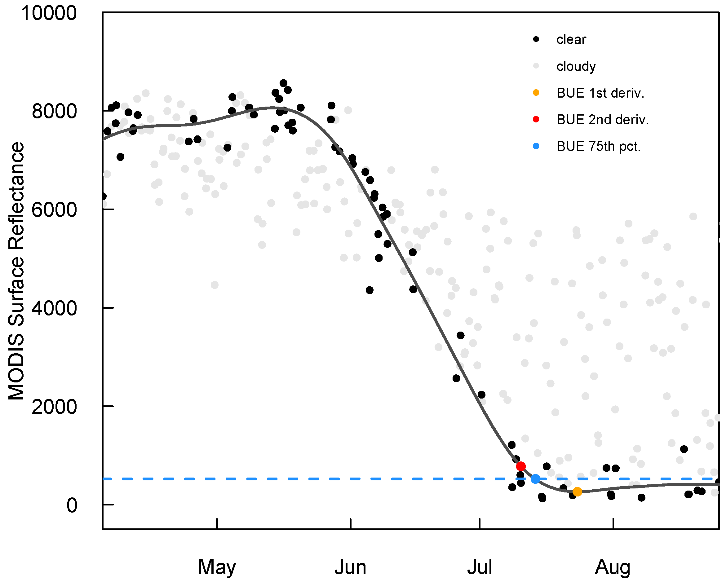
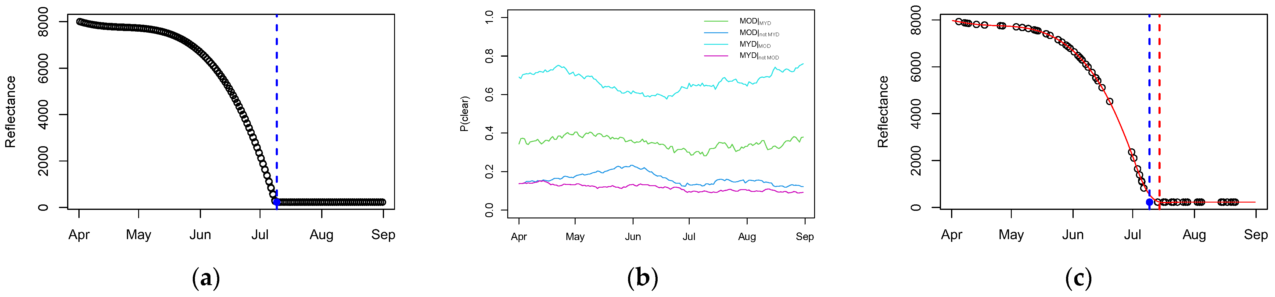
2.3.2. Lake Ice Phenology from MODIS

For simplicity in comparison to in-situ lake ice timing data, the MODIS surface reflectance from band 3 was averaged over the entire lake surface for each satellite overpass. This was accomplished by drawing a polygon in Google Earth Engine that matched the boundary of the lake, and then averaging the MODIS reflectance data within the polygon. Thus, each overpass was treated as a single value in order to create a time series of mean lake surface reflectance (Figure 4). The lake-wide mean MODIS surface reflectance time series also showed a seasonal pattern, with generally higher reflectance in the winter (when the lake surface was covered with snow and ice) and lower reflectance in the summer (when the lake surface consisted of less reflective open water). This difference allowed for identification of BUE as the end of the transition period from the high winter reflectance to lower summer reflectance.

Unfortunately, the MODIS reflectance product was not available after late September each year, presumably due to low levels of reflected light as the Arctic transitioned toward polar night. Freeze-up of Linnévatnet did not occur until October or later, so it was not possible to observe FUE using MODIS.

The frequencies of electromagnetic radiation observed by MODIS do not penetrate through clouds. Cloud cover added considerable noise to this seasonal reflectance pattern because clouds were present throughout the year and their reflectance was usually in between the low reflectance of open water and the high reflectance of snow and ice. Unfortunately, we found that the MODIS internal cloud algorithm flag was not completely effective at filtering out cloudy days, probably due to the difficulty of distinguishing clouds from lake ice and snow, as well as partial cloud cover. So, we manually filtered out cloudy MODIS observations by viewing the MODIS data on Google Earth Engine Explorer. When the outline of the lake (either ice-free or ice-covered) was visible, the data were identified as cloudless, while images where the lake was obscured were discarded. This resulted in a time series of cloud-free MODIS surface reflectance observations, but with many gaps due to missing data (~75–80%).

In order to provide the most accurate BUE and FUE dates possible, it was necessary to fill the gaps in the time series. We tested multiple gap-filling methods, including linear interpolation, logistic curves, kernel smoothers, and splines. Ultimately, we found that a cubic smoothing spline (“smooth.spline” in R) was effective at retaining the features of the MODIS time series without overfitting the data. Smoothing parameters were calculated using ordinary leave-one-out cross-validation.

We tested three automated methods (described below) to identify BUE from the smoothing spline fit to cloud-free, lake-wide mean surface reflectance (i.e., a smoothed, gap-filled representation of the time series). These included (1) identifying the first date at the bottom of the downward trend in the smoothing spline, where the first derivative was equal to zero (i.e., first location where the spline leveled out in the early summer; hereafter the “MODIS dSR” method); and (2) the date nearest to the bottom of the spline trend where the second derivative was equal to zero (i.e., point of maximum curvature; hereafter the “MODIS d²SR” method). Additionally, we found (3) the earliest date in each year where the smoothing spline crossed below a reflectance threshold, calculated as the third quartile (i.e., 75th percentile) of the clear sky MODIS surface reflectance values during the summer (20 July–31 August) of the given year (hereafter, the “MODIS Summer Q₃” method). The mid-July through August period was chosen as it was a consistent annual period of open water on the lake, before some high surface reflectance values in the fall (presumably due to sun angle dynamics).

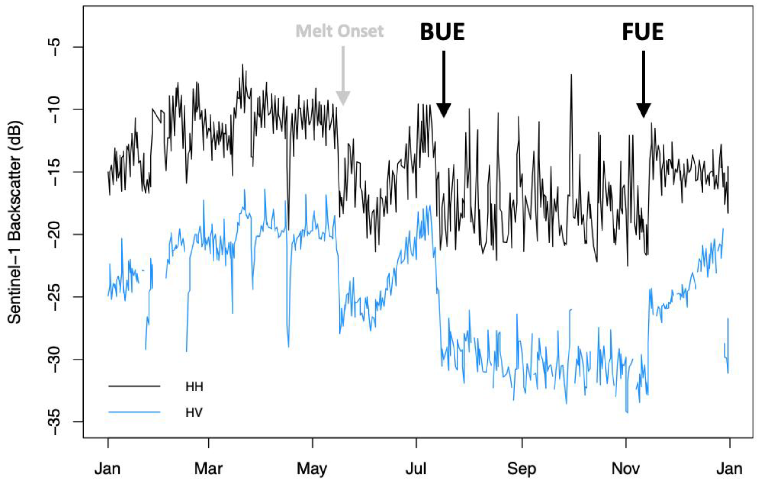
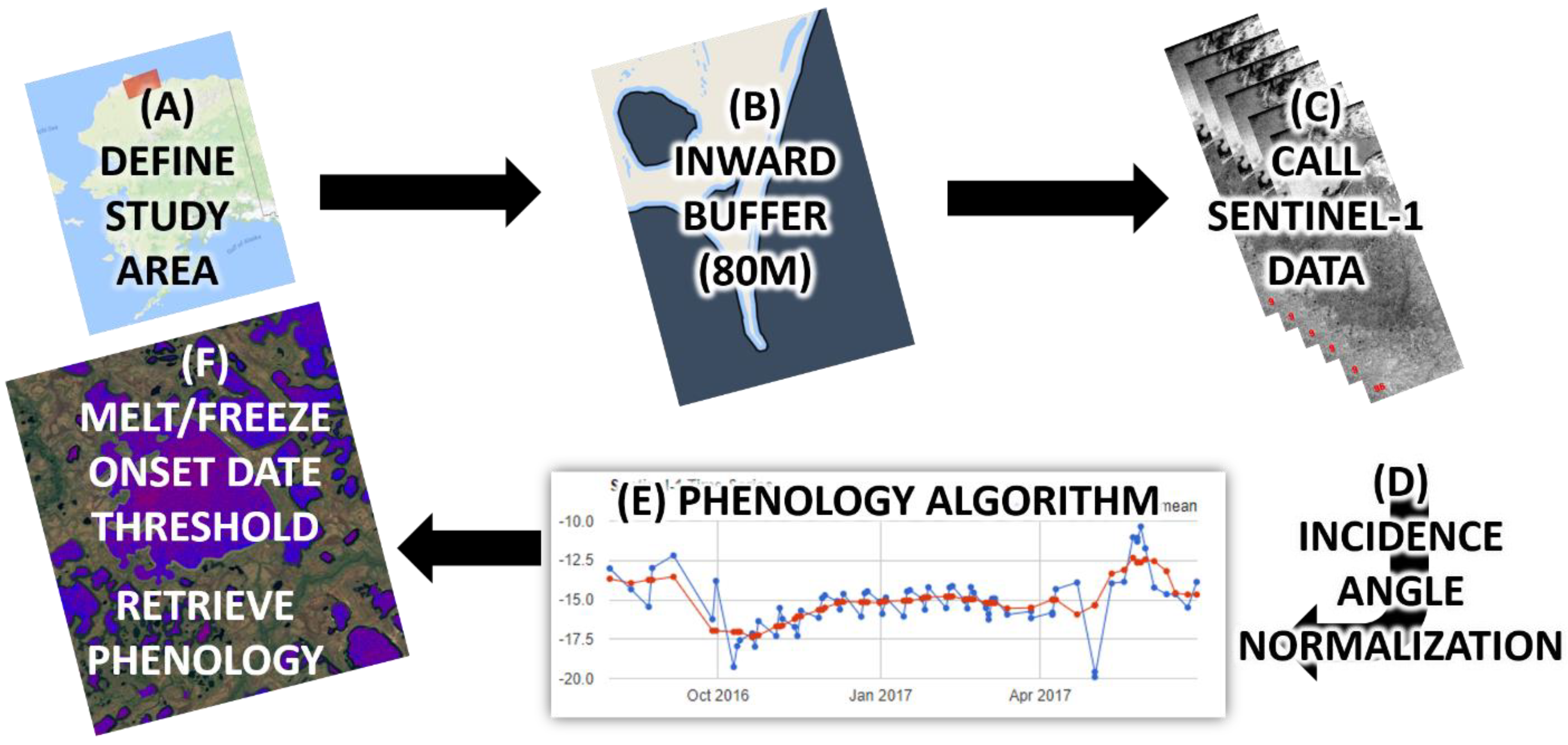
2.3.3. Lake Ice Phenology from Sentinel-1

Similar to the processing of the MODIS data, Google Earth Engine was used to create a lake-wide average time series of Sentinel-1 backscatter, where the HH and HV polarizations (and incidence angle) were averaged separately over the entire lake surface in order to create a backscatter time series for each polarization.

For the Sentinel-1 backscatter, an angular dependence was observed. Higher backscatter values were observed at lower incidence angle (i.e., the angle between the radiation emitted from the instrument and the ground surface), which introduced variability into the time series that made it more difficult to interpret. So, a simple regression-based normalization was applied to the Sentinel-1 backscatter data in order to reduce angle-based noise in the data. First, we smoothed the backscatter times series using locally estimated scatterplot smoothing (LOESS), a local regression smoothing method, in order to approximate the seasonal evolution of lake backscatter properties. Then, the moving average was subtracted from the original backscatter times series to obtain a time series of residuals (which were partly a function of incidence angle). The incidence angle was regressed on the backscatter residuals using simple linear regression to obtain a statistical relationship between residual and incidence angle (R² = 0.63 for HH and 0.54 for HV). Then, this linear relationship was used to predict an expected backscatter residual time series based on the known incidence angles. The regression-predicted backscatter residual was subtracted from the observed backscatter residuals in order to remove the expected effect of incidence angle on backscatter. Finally, this difference was added to the moving average backscatter to obtain an incidence angle-corrected backscatter time series. The method was applied separately to the HH and HV polarizations. This correction method is imperfect, as a higher influence of backscatter was observed during periods of open water as compared to ice cover, but it did help to reduce noise in the time series and achieved the main purpose of increasing the interpretability of the backscatter time series. During the ice-covered time periods, the normalization of backscatter over incidence angle is appropriate for lake ice as the dominant scattering mechanism observed in shallow lake ice is single-bounce interactions occurring at the ice–water interface [58].

The incidence angle-corrected, lake-wide mean Sentinel-1 backscatter showed a seasonal pattern (Figure 5), but it was different from that of MODIS. Generally, the backscatter increased throughout the winter, followed by a sharp drop in the spring. This drop was followed by a gradual increase and then another sharp drop in the early summer. During the summer, the backscatter magnitude remained generally lower than the rest of the year (but also with high variability). Finally, the backscatter increased, sometimes gradually and sometimes abruptly, in the fall into winter. Based on previous studies (e.g., [36,59]), we interpret the first sharp drop in backscatter in the spring to indicate the first melting of the snow and lake ice (i.e., break-up start—BUS) which leads to absorption of the incident microwave signal, while the second drop (which was followed by low backscatter throughout the summer) indicates the disappearance of ice from the lake (BUE), resulting in a smooth water surface that reflects incident microwaves away from the sensor. Due to the difficulty in identifying the individual dates of these features (because of noise in the time series), we identified the BUE date manually from both HH and HV polarizations as the last date of the second drop in backscatter (hereafter, the “S1 HH Manual” and “S1 HV Manual” methods). FUE dates were identifiable by a decrease in the variability of the backscatter values over time in the HH polarization, likely due to more diffuse scattering from ice or snow on the lake surface, as compared with open water. However, this change in backscatter variability was not easily distinguishable in the HV polarization.

An automated algorithm to estimate freeze onset from Sentinel-1 was also used, which could be broadly applied in other regions to determine lake ice phenology. This method is illustrated with a flow diagram in Figure 6. The process is as follows: In Google Earth Engine, the Sentinel-1 A/B repository is called and filtered for the desired time periods (typically a one-year period (e.g., from 1 August 2017 to 30 July 2018) (Figure 6A). Filters are applied to ensure acquisition property consistency throughout the time series with respect to orbit path, imaging mode, and polarization. For the purpose of this study, the filters applied were that all images had to be acquired in Interferometric Wideswath (IW) mode using HH co-polarization. For Linnévatnet, Sentinel-1 acquisitions were acquired on the same orbit track, which did not necessitate the normalization of backscatter for multiple incidence angles.

Once the repository is queried, an image collection of all filtered images is produced with a 40 m spatial resolution. An image stack is then generated to allow for the tracking of backscatter over time (Figure 6C). Recent understanding of microwave interactions with freshwater ice has indicated the source of backscatter is surface roughness at the ice–water interface, allowing for the normalization of backscatter, following [60,61] (Figure 6D). A time series of backscatter is generated for each pixel, and a smoothing algorithm is applied. The smoothing algorithm extracts the mean value for pixels acquired within five days before or after the initial acquisition to capture variability of incidence angle, and orbit path without including repeat passes. The approach of averaging the most recent acquisitions is not used because some periods and regions in this study occasionally do not have dense enough coverage to include those acquisitions without incorporating repeat passes, which would limit the observation of change in backscatter due to thermodynamic shifts. A user-defined threshold is set to monitor all drops in the smoothed backscatter time series for each pixel, with the timing of any drops flagged and recorded (Figure 6E). For consistency from year to year, the date of the first backscatter drop greater than 5 dB—in this case for the smoothed time series—is extracted and is recorded as the timing of freeze- or melt-onset for that pixel within the lake boundary (Figure 6F). Below, we report the median freeze onset date for all 40 m pixels within the lake boundary, for comparison to other freeze-up estimates (hereafter, the “S1 Auto Median” method).

2.3.4. Agreement between Lake Ice Phenology Estimates

To assess the viability of the satellite-derived BUE estimates, we calculated agreement statistics between the satellite-derived BUE estimates and the in-situ BUE estimates. These statistics included bias, mean absolute error (MAE), and root mean squared error (RMSE). Agreement statistics were computed for each different combination of satellite and in-situ methods, treating the BUE values from each individual year as a data pair. We followed the same procedure to calculate agreement statistics for FUE. Additionally, we calculated agreement statistics between the two in-situ methods (camera images and water temperature) for each of BUE and FUE.

3. Results

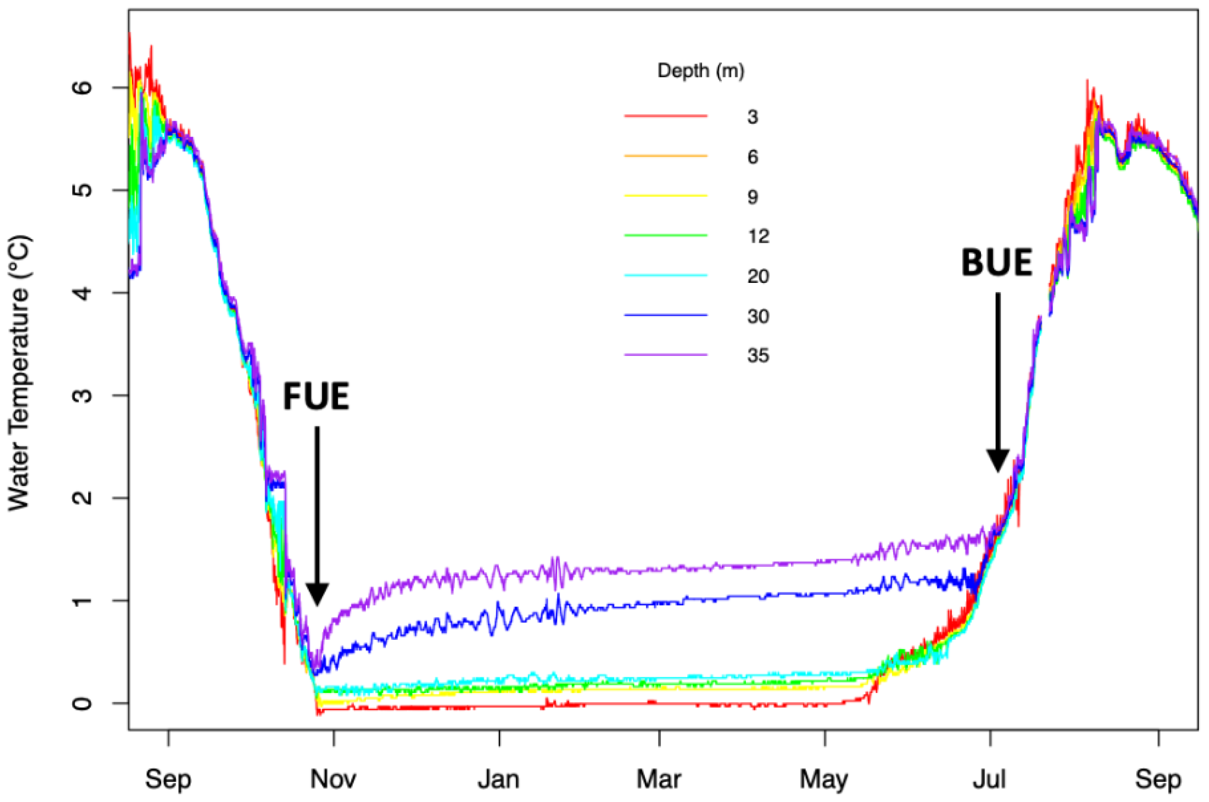
3.1. Lake Water Temperature Dynamics

Considerable annual variability was observed in both mean lake water temperature throughout the summer and in the degree of water temperature stratification during the winter. However, a general increasing trend in lake temperature is evident in Figure 7, with warmer years clustered in the later portion of the time series. The mean water temperature from June–November (DOY 152–334) showed a significant increasing trend of 0.06 °C per year, according to a Theil–Sen line fit to the data (Mann–Kendall (M-K) trend test: p = 0.008). Additionally, the lake stayed warm for a longer period each year. The latest day with a mean temperature above 4 °C was found for each year, and significant increasing trend of 1 day per year was observed (Theil–Sen line; M-K test: p = 0.012). Similar significant trends were found for 3 °C and 2 °C. These findings are consistent with extensive literature that documents rapid Arctic warming in the past two decades [26,62].

3.2. In-Situ Observations of Lake Ice Timing

BUE and FUE dates from the automated photographs of the lake surface, and inferred from lake water temperature, showed that BUE did not change significantly from 2004 to 2019 (M-K trend test on water temperature BUE estimates: p = 0.30) (Figure 8). While Svalbard lies far off the northern European coast, this is consistent with findings of little change in BUE in Northern Europe [23]. In contrast, the FUE date was observed to occur much later in recent years as compared with the mid-2000s, and there is much more year-to-year variability. The mean FUE from 2003–2007 was day-of-year (DOY) 294, while the mean FUE from 2015–2019 was DOY 314, based on lake water temperature FUE estimates. This corresponded to an increase of 1.5 days per year over the period 2003–2019, according to a Theil–Sen line fit to the data (M-K test: p = 0.002). These findings are consistent with a rise in winter air temperatures in Svalbard [52]. Mainly due to the later freeze-up, there was an increase in the annual period of open water of approximately 1.4 days per year from 2003 to 2019 (Theil–Sen line; M-K test: p = 0.01). While the 16-year period of this study is less than the commonly accepted 30-year period to define climate normals, our findings are consistent with trends in the lake water temperature and with extensive observations of rapid Arctic warming [26,62].

The agreement in ice timing between the two in-situ methods (photographs and lake water temperature profiles) is comparable for FUE dates and BUE dates, but depends on which view of the lake is considered. The RMSE for FUE, identified manually from water temperature dynamics (“WTemp Manual” method), is 2.6 and 5.3 days for the North and Plume cameras, respectively, while the RMSE for BUE dates is 3.0 and 3.5 days, respectively (see

Table 1. Agreement between BUE dates from the camera images and other BUE estimation methods.

Data	Method 1	North Camera (n = 6)			Plume Camera (n = 8)
		Bias (Days)	MAE (Days)	RMSE (Days)	Bias (Days)	MAE (Days)	RMSE (Days)
In-situ water temp.	Manual	−0.5	2.64	3.0	−0.9	3.3	3.5
MODIS	dSR	4.5	5.3	6.7	2.9	4.5	5.6
	d2SR	−3.9	4.6	4.9	−5.7	6.3	6.9
	Summer Q3	−1.3	2.4	2.5	−2.3	3.2	3.5
Sentinel-1 2	HH Manual	1.4	2.0	2.2	1.0	2.0	2.2
	HV Manual	1.4	1.4	1.8	1.5	1.5	2.1

¹ The various BUE identification methods are described in Section 2.3.1, Section 2.3.2 and Section 2.3.3. ² The statistics for Sentinel-1 are based on very few data pairs (n = 3 for North camera, n = 2 for Plume camera) due to loss of camera images in 2017–2019 (see Figure 8a).

and

Table 2. Agreement between FUE dates from the camera images and other FUE estimation methods.

Data	Method 1	North Camera (n = 8)			Plume Camera (n = 12)
		Bias (Days)	MAE (Days)	RMSE (Days)	Bias (Days)	MAE (Days)	RMSE (Days)
In-situ water temp.	Manual	−2.0	2.5	3.3	2.1	3.1	5.3
	AnnMin	−1.3	1.5	2.3	3.3	3.5	6.2
Sentinel-1 2	HV Manual	−1.6	4.7	5.2	8.8	10.6	12.9
	Auto Median	0.4	5.7	6.7	13.5	13.5	15.2

¹ The various FUE identification methods are described in Section 2.3.1, Section 2.3.2 and Section 2.3.3. ² The statistics for Sentinel-1 are based on very few data pairs (n = 3 for each camera) due to loss of camera images in 2016, 2018, and 2019 (see Figure 8b).

). FUE estimates from the annual minimum in water column temperature (“WTemp AnnMin” method) resulted in a RMSE of 2.3 days with the North camera, but 6.2 days with the Plume camera. This difference can likely be attributed to the fact that the North camera view includes a much broader view of the lake surface and also contains mooring G (which is the source of the water temperatures in this analysis), while the Plume camera observes a very small portion of the lake that also does not contain mooring G. It is somewhat surprising that BUE can be identified with comparable error to FUE, mainly because it can be difficult to identify the BUE from the lake water temperature profiles due to gradual mixing of the lake in the spring and early summer, while it is straightforward to observe ice disappearance from the photographs. For FUE, both methods have highly identifiable transitions, and thus good agreement, except in years when FUE occurs late in the fall. In those cases, light levels are low, and it can be hard to distinguish open water from ice cover in the photographs, so we sometimes relied on snow accumulation on the lake surface to indicate the presence of ice. This may have introduced error into FUE camera estimates. The FUE transition is very identifiable from the lake water temperatures because it is marked by the beginning of winter-long stratification of water temperature within the lake. This is evident in the good agreement between the manual FUE estimates (“WTemp Manual”), which used the stratification dynamics to identify FUE, and the FUE estimates from the annual minimum in water column temperature (“WTemp AnnMin”; MAE = 1.6 days, RMSE = 2.0 days; see Table 4).

3.3. Satellite vs. In-Situ Lake Ice Phenology

The agreement between the different satellite methods and the in-situ methods varies by sensor, method, and transition (BUE vs. FUE). Agreement statistics are provided in Table 1, Table 2,

Table 3. Agreement between manual BUE dates from water temperature dynamics (the “WTemp Manual” method) and other BUE estimation methods (n = 16).

Data	Method 1	Bias (Days)	MAE (Days)	RMSE (Days)
MODIS	dSR 2	8.4	8.7	11.4
	d2SR 3	−4.0	4.7	5.5
	Summer Q3	2.0	4.0	5.5
Sentinel-1 4	HH Manual	2.6	3.1	3.4
	HV Manual	2.4	2.9	3.2

¹ The various BUE identification methods are described in Section 2.3.1, Section 2.3.2 and Section 2.3.3. ² For the year 2005, the smoothing spline fit to the MODIS surface reflectance did not reach a slope of zero as it declined through the melt period, so a BUE date could not be calculated. Thus, n = 15 for this method. ³ For the year 2006, the second derivative of the smoothing spline was not calculated. Thus, n = 15 for this method. ⁴ The statistics for Sentinel-1 are based on n = 5 data pairs (see Figure 8a).

and

Table 4. Agreement between manual FUE dates from water temperature dynamics (the “WTemp Manual” method) and other FUE estimation methods (n = 16).

Data	Method 1	Bias (Days)	MAE (Days)	RMSE (Days)
In-situ water temp.	AnnMin	0.9	1.6	2.0
Sentinel-1 2	HV Manual	3.4	3.8	5.2
	Auto Median	14.0	16.4	23.3

¹ The various FUE identification methods are described in Section 2.3.1, Section 2.3.2 and Section 2.3.3. ² The statistics for Sentinel-1 are based on n = 5 data pairs (see Figure 8b).

.

For BUE, Sentinel-1 outperformed MODIS in terms of agreement with the in-situ observations, with MAE of 1.4–3.1 days and RMSE of 1.8–3.4 days among the BUE estimation method and in-situ combinations (i.e., cameras and water temperature). For MODIS, BUE agreement ranged from MAE of 2.5–8.7 days and RMSE ranged from 2.5 to 11.4 days among the BUE estimation methods and cameras. However, the Sentinel-1 statistics are based on a very small sample size (n = 5 for comparison to water temperature BUE dates, and n = 3 for North camera and n = 2 for Plume camera due to loss of camera images in 2017–2019). Of the MODIS methods, the “Summer Q3” method (which determined BUE based on when the smoothing spline fit to the surface reflectance data crossed below a threshold equal to the 75th percentile of open-water surface reflectance) showed the best agreement, with MAE of 2.4–4.0 days and RMSE of 2.5–5.5 days among the different in-situ comparisons.

The agreement between the Sentinel-1 and the in-situ FUE estimates was worse than for BUE, with MAE of 3.8–13.6 days and RMSE of 5.2–23.3 days (Table 2 and Table 4). However, some of this disagreement can be contributed to the difficulty in identifying the FUE transition in the camera images in recent years due to later freeze-up, as well as small sample size for the comparison (n = 3 for both cameras due to loss of images in 2016, 2018, and 2019). The agreement with manual FUE estimates from water temperature dynamics, which did not suffer from those limitations, was better than with either camera (MAE = 3.8 days; RMSE = 5.2 days for manual HV FUE estimates). The larger disagreement between the Sentinel-1 “Auto Median” method and the water temperature FUE estimates is largely driven by a large difference in 2019. Without this, the MAE and RMSE decrease to 8.3 and 8.9 days, respectively. FUE could not be calculated from MODIS surface reflectance due to the low light levels during fall freeze-up.

4. Discussion

4.1. Considerations for Determining Lake Ice Timing

In this analysis, we identified a single date each year where the lake became completely ice-free in the spring (BUE) and a single date where the lake became completely ice-covered in the fall (FUE), remaining ice-covered for the rest of the winter. However, it is important to note that the break-up of ice in the spring and freeze-up in the fall are not instantaneous processes. A recent synthesis article [2] noted this limitation and highlighted that moving from binary to continuous monitoring of lake ice is a path to advance lake ice research through interdisciplinary collaboration. The process of spring melting of lake ice (and the snow that may cover it) can take over a month. This is evident in both the Sentinel-1 time series, in which a date of first spring melting can often be identified (see Figure 5), as well as the MODIS surface reflectance time series, which shows a decrease in surface reflectance that lasts a month or more (Figure 4). Additionally, the period over which ice disappears from the lake surface to reveal open water can last over a week, with fragmented ice cover being blown back and forth over the lake surface by the wind. This gradual ice breakup period averaged 7–8 days for the years with automatic camera images of the lake. For this analysis, we have chosen the most identifiable events in the lake ice break-up and freeze-up processes (BUE and FUE, respectively), but it is important to consider that distilling gradual processes into individual points in time (or binary: ice vs. no ice) may introduce some amount of uncertainty. This uncertainty may be reflected in the level of agreement between the satellite and in-situ ice timing estimates.

4.2. Effect of Clouds on MODIS BUE Dates

In order to interpret the level of agreement between the BUE dates from MODIS and the BUE dates from in-situ observations, we conducted an additional simulation. The goal of the simulation was to evaluate the effect of data loss due to cloud cover on MODIS BUE estimates, because the lake surface was not visible on cloudy days and the MODIS data on those days were discarded.

First, all MODIS surface reflectance observations (both MOD09GA and MYD09GA) of the lake on cloudless days for the entire 16-year time series were plotted as a function of decimal day of year (April–August), with the Terra and Aqua observations plotted according to their overpass times (10:30 and 13:30 local time, respectively). Then, an idealized MODIS seasonal pattern was generated by fitting a 10th degree polynomial function to the MODIS observations from winter until the annual mean BUE date (7 July), and all days after 7 July were assigned a constant value equal to the mean reflectance for the remainder of the summer. The result was an idealized time series of alternating Terra and Aqua MODIS observations (10:30 and 13:30 local time, respectively) for Linnévatnet for each day of the year from 1 April–31 August, as shown in Figure 9a.

Next, the cloud cover for the lake was modeled as a Markov process. For each day of the year (in a 31-day moving window across all years), the probability of observing a clear (i.e., not cloudy) day was calculated, dependent on (1) whether the previous observation was cloudy or clear, and (2) whether the previous observation was from the Terra or Aqua MODIS instrument. This second condition was deemed necessary because the Aqua instrument observes the lake only 3 h after the Terra instrument, but there are 21 h between Aqua and Terra observations. The average probability of a clear day from April–August was 0.21 for Terra and 0.23 for Aqua, reinforcing the idea that clouds are very common in this Arctic maritime location. The probability of observing a clear day was also highly dependent on whether the previous observation was cloudy or clear (see Figure 9b), indicating a high degree of persistence in cloud conditions.

This Markov transition matrix was then used to randomly generate time series of cloudy vs. clear observations, which was applied to the idealized MODIS time series. For each cloudy observation, the value from the idealized times series was replaced with a missing value, resulting in a time series where the data were randomly knocked out due to simulated clouds (see Figure 9c). This process was repeated 1000 times, generating 1000 simulated times series of cloud-impacted MODIS observations. Then, a smoothing spline was independently fit to each simulated time series, using the same method that was used for the MODIS observations (Section 2.3.2), and BUE dates were calculated according to the MODIS “dSR” and “Summer Q₃” methods (Section 2.3.2). These BUE dates were then averaged across all 1000 simulations of data loss due to cloud cover. Finally, the simulated BUE dates were compared to the “known” BUE date from the simulated time series (July 7 at 16:00 local time), in order to evaluate the uncertainty introduced into the MODIS BUE identification method due to cloud cover.

The RMSE between the “known” BUE date and the mean BUE date from the simulations was 3.0 days for the “Summer Q₃” method, and 4.4 days for the “dSR” method. The MAE for the two methods were 1.8 and 3.3 days, respectively. These simulation results show that the error in estimated BUE dates due to data loss from cloud cover is of similar magnitude to the error between observed BUE dates from the in-situ data and estimated BUE dates from MODIS (Table 1 and Table 3). Thus, it is reasonable to assume that a large majority of the error in the MODIS-derived BUE dates is due to loss of data due to cloud cover, rather than flaws in the methodology or MODIS observations. This lends confidence to the ability of MODIS to accurately observe lake ice conditions in clear conditions. The accuracy of the BUE dates from MODIS will thus be primarily dependent on the frequency of cloud cover at a given location (where fewer clouds will result in more accurate BUE dates), as well as the accuracy of cloud masking over ice and snow surfaces.

4.3. Lake Ice Phenology from MODIS vs. Sentinel-1

The results of this analysis showed that both MODIS and Sentinel-1 were reasonably accurate in determining the date of ice disappearance (i.e., BUE date) for a large Arctic lake. These findings lend confidence to remote sensing of lake ice phenology, consistent with previous studies that used ground-based observations for validation [12,19,23,39,40]. Sentinel-1 was slightly more accurate in determining BUE (Table 1). This difference can be attributed to the fact that electromagnetic radiation penetrates through clouds at the microwave frequency of Sentinel-1, but does not penetrates through clouds at the optical frequencies of MODIS. Thus, Sentinel-1 did not suffer loss of data due to cloud cover, while nearly 80% of MODIS observations were discarded due to clouds. A large portion of the error in Sentinel-1 BUE estimates can likely be attributed to differing scattering properties at different view angles. A simple method was used in this manuscript to reduce these errors, but a more sophisticated method may improve the accuracy of BUE date identification from Sentinel-1.

FUE was more difficult to identify than BUE using satellite observations. MODIS surface reflectance observations were not available during FUE due to low light levels during the polar night. Based on in-situ observations, most FUE dates occurred in late October, with no FUE dates before October 16th, while MODIS reflectance decreased to extremely low values after approximately October 10th each year and thus were not interpretable. Sentinel-1 observations were available year-round, but the fall freeze-up was less identifiable in the backscatter time series than for spring break-up. This led to a large amount of uncertainty in FUE dates (RMSE of at least 5.2 days). This uncertainty may partially be due to the gradual nature of freeze-up, punctuated freezing interrupted by melting (and thus mixed, snow, ice, and liquid water), or deformation features [35,36]. The greater uncertainty in satellite FUE estimates is unfortunate because the fall freeze-up is when the most long-term change is observed for Linnévatnet. The Arctic is a remote region, so satellite observations are important for tracking indicators of climate change. Numerous ground-based studies have documented later freeze-up and earlier break-up of lake ice across northern latitudes, and remote sensing has corroborated trends in earlier break-up (e.g., [20,23]). However, the slightly larger uncertainty in Sentinel-1 FUE estimates, combined with the relatively short Sentinel-1 record, may make it difficult to confidently identify trends in FUE. Additionally, trends in FUE for some high Arctic lakes may have gone unobserved by optical satellites over the past two decades due to low light levels in the fall [23].

Despite the complication of low light levels in the fall at high latitudes, the identification of ice phenology from both the Sentinel-1 and MODIS benefitted from the high latitude of the study site combined with the polar orbits of the satellites, as well as the fact that each instrument is flown on two satellite platforms (Sentinel-1A and Sentinel-1B, and Terra and Aqua, respectively). These factors resulted in high frequency observations of the study area (1 day or less for Sentinel-1 and at least twice daily for MODIS). However, the frequency of overpasses for both Sentinel-1 and MODIS will decrease at lower latitudes. This effect is most pronounced for Sentinel-1 because MODIS has a much wider observation swath. While Sentinel-1 outperformed MODIS for Linnévatnet, it is possible (or even likely) that MODIS will be more useful for determining ice timing at lower latitudes, where Sentinel-1 overpass frequency decreases significantly (every 6 days over much of the continents outside of Europe) and the amount of sunlight received in the fall increases (making identification of FUE possible). Similarly, Sentinel-1 overpasses are less frequent outside of the European Arctic, with revisit frequency decreasing to 1–4 days. Additionally, Sentinel-1 operates at different polarizations over the Arctic (HH and HV) than over much of the rest of the Earth’s surface (VV and VH), which could affect the detectability of the features in the backscatter time series that were used infer lake ice phenology in this analysis. Lastly, MODIS benefits from a longer history of observations as compared to Sentinel-1 (year 2000 to present for MODIS vs. 2014 to present for Sentinel-1), so MODIS is most useful for evaluating longer-term trends in climate indicators.

In summary, this case study suggests that optical and SAR satellite data can be confidently used to monitor lake ice changes in the High Arctic, and at regional scales across the Arctic, with some sensor-specific considerations. However, lake-specific conditions (e.g., size, depth, orientation, and hydrology) may influence individual lake melt-out and freeze-up processes and the ability to detect ice phenology from satellite imagery.

References

1. Serreze, M.C.; Barry, R.G. Processes and impacts of Arctic amplification: A research synthesis. Global Planet. Change 2011, 77, 85–96. [Google Scholar] [CrossRef]
2. Sharma, S.; Meyer, M.F.; Culpepper, J.; Yang, X.; Hampton, S.; Berger, S.A.; Brousil, M.R.; Fradkin, S.C.; Higgins, S.N.; Jankowski, K.J.; et al. Integrating perspectives to understand lake ice dynamics in a changing world. J. Geophys. Res.-Biogeo. 2020, 125, e2020JG005799. [Google Scholar] [CrossRef]
3. Sharma, S.; Richardson, D.C.; Woolway, R.I.; Imrit, M.A.; Bouffard, D.; Blagrave, K.; Daly, J.; Filazzola, A.; Granin, N.; Korhonen, J.; et al. Loss of ice cover, shifting phenology, and more extreme events in Northern Hemisphere lakes. J. Geophys. Res.-Biogeo. 2021, 126, e2021JG006348. [Google Scholar] [CrossRef]
4. Goosse, H.; Kay, J.E.; Armour, K.C.; Bodas-Salcedo, A.; Chepfer, H.; Docquier, D.; Jonko, A.; Kushner, P.J.; Lecomte, O.; Massonnet, F.; et al. Quantifying climate feedbacks in polar regions. Nat. Commun. 2018, 9, 1919. [Google Scholar] [CrossRef]
5. Williamson, C.E.; Dodds, W.; Kratz, T.K.; Palmer, M.A. Lakes and streams as sentinels of environmental change in terrestrial and atmospheric processes. Front. Ecol. Environ. 2008, 6, 247–254. [Google Scholar] [CrossRef]
6. Adrian, R.; O’Reilly, C.M.; Zagarese, H.; Baines, S.B.; Hessen, D.O.; Keller, W.; Livingstone, D.M.; Sommaruga, R.; Straile, D.; van Donk, E.; et al. Lakes as sentinels of climate change. Limnol. Oceanogr. 2009, 54, 2283–2297. [Google Scholar] [CrossRef] [PubMed]
7. Weyhenmeyer, G.A.; Meili, M.; Livingstone, D.M. Nonlinear temperature response of lake ice breakup. Geophys. Res. Lett. 2004, 31, L07203. [Google Scholar] [CrossRef] [Green Version]
8. Walsh, J.E.; Anisimov, O.; Hagen, J.O.; Jakobsson, T.; Oerlemans, J.; Prowse, T.D.; Romanovsky, V.; Savelieva, N.; Serreze, M.; Shiklomanov, A.; et al. Cryosphere and hydrology. In Arctic Climate Impact Assessment. Scientific Report; Arris, L., Ed.; Cambridge University Press: Cambridge, UK, 2005; pp. 183–242. [Google Scholar]
9. Higgins, S.N.; Desjardins, C.M.; Drouin, H.; Hrenchuk, L.E.; Van der Sanden, J.J. The role of climate and lake size in regulating the ice phenology of boreal lakes. J. Geophys. Res.-Biogeo. 2021, 126, e2020JG005898. [Google Scholar] [CrossRef]
10. Liston, G.E.; Hall, D.K. An energy-balance model of lake-ice evolution. J. Glaciol. 1995, 41, 373–382. [Google Scholar] [CrossRef] [Green Version]
11. Brown, L.C.; Duguay, C.R. The response and role of ice cover in lake-climate interactions. Prog. Phys. Geog. 2010, 34, 671–704. [Google Scholar] [CrossRef]
12. Arp, C.D.; Jones, B.M.; Grosse, G. Recent lake ice-out phenology within and among lake districts of Alaska, USA. Limnol. Oceanogr. 2013, 58, 2013–2028. [Google Scholar] [CrossRef]
13. Prowse, T.; Alfredsen, K.; Beltaos, S.; Bonsal, B.R.; Bowden, W.B.; Duguay, C.R.; Korhola, A.; McNamara, J.; Vincent, W.F.; Vuglinsky, V.; et al. Effects of changes in arctic lake and river ice. Ambio 2011, 40, 63–74. [Google Scholar] [CrossRef] [Green Version]
14. Dibike, Y.; Prowse, T.; Saloranta, T.; Ahmed, R. Response of Northern Hemisphere lake-ice cover and lake-water thermal structure patterns to a changing climate. Hydrol. Process. 2011, 25, 2942–2953. [Google Scholar] [CrossRef]
15. Hampton, S.E.; Galloway, A.W.; Powers, S.M.; Ozersky, T.; Woo, K.H.; Batt, R.D.; Labou, S.G.; O’Reilly, C.M.; Sharma, S.; Lottig, N.R.; et al. Ecology under lake ice. Ecol. Lett. 2017, 20, 98–111. [Google Scholar] [CrossRef] [PubMed]
16. Dugan, H.A. A Comparison of ecological memory of lake ice-off in eight north-temperate lakes. J. Geophys. Res.-Biogeo. 2021, 126, e2020JG006232. [Google Scholar] [CrossRef]
17. Magnuson, J.J.; Robertson, D.M.; Benson, B.J.; Wynne, R.H.; Livingstone, D.M.; Arai, T.; Assel, R.A.; Barry, R.G.; Card, V.; Kuusisto, E.; et al. Historical trends in lake and river ice cover in the Northern Hemisphere. Science 2000, 289, 1743. [Google Scholar] [CrossRef] [PubMed] [Green Version]
18. Duguay, C.R.; Prowse, T.D.; Bonsal, B.R.; Brown, R.D.; Lacroix, M.P.; Ménard, P. Recent trends in Canadian lake ice cover. Hydrol. Process. 2006, 20, 781–801. [Google Scholar] [CrossRef]
19. Latifovic, R.; Pouliot, D. Analysis of climate change impacts on lake ice phenology in Canada using the historical satellite data record. Remote Sens. Environ. 2007, 106, 492–507. [Google Scholar] [CrossRef]
20. Prowse, T.; Alfredsen, K.; Beltaos, S.; Bonsal, B.; Duguay, C.; Korhola, A.; McNamara, J.; Pienitz, R.; Vincent, W.F.; Vuglinsky, V.; et al. Past and future changes in Arctic lake and river ice. Ambio 2011, 40, 53–62. [Google Scholar] [CrossRef] [Green Version]
21. Benson, B.J.; Magnuson, J.J.; Jensen, O.P.; Card, V.M.; Hodgkins, G.; Korhonen, J. Extreme events, trends, and variability in Northern Hemisphere lake-ice phenology (1855–2005). Clim. Change 2012, 112, 299–323. [Google Scholar] [CrossRef]
22. O’Reilly, C.M.; Sharma, S.; Gray, D.K.; Hampton, S.E.; Read, J.S.; Rowley, R.J.; Schneider, P.; Lenters, J.D.; McIntyre, P.B.; Kraemer, B.M.; et al. Rapid and highly variable warming of lake surface waters around the globe. Geophys. Res. Lett. 2015, 42, 10–773. [Google Scholar] [CrossRef] [Green Version]
23. Šmejkalová, T.; Edwards, M.E.; Dash, J. Arctic lakes show strong decadal trend in earlier spring ice-out. Sci. Rep. 2016, 6, 38449. [Google Scholar] [CrossRef] [PubMed]
24. Griffiths, K.; Michelutti, N.; Sugar, M.; Douglas, M.S.; Smol, J.P. Ice-cover is the principal driver of ecological change in High Arctic lakes and ponds. PLoS ONE 2017, 12, e0172989. [Google Scholar] [CrossRef] [PubMed]
25. Lehnherr, I.; Louis, V.L.S.; Sharp, M.; Gardner, A.S.; Smol, J.P.; Schiff, S.L.; Muir, D.C.G.; Mortimer, C.A.; Michelutti, N.; Tarnocai, C.; et al. The world’s largest High Arctic lake responds rapidly to climate warming. Nat. Comm. 2018, 9, 1290. [Google Scholar] [CrossRef] [PubMed]
26. Newton, A.M.W.; Mullan, D.J. Climate change and Northern Hemisphere lake and river ice phenology from 1931–2005. Cryosphere 2021, 15, 2211–2234. [Google Scholar] [CrossRef]
27. Post, E.; Alley, R.B.; Christensen, T.R.; Macias-Fauria, M.; Forbes, B.C.; Gooseff, M.N.; Iler, A.; Kerby, J.T.; Laidre, K.L.; Mann, M.E.; et al. The polar regions in a 2 C warmer world. Sci. Adv. 2019, 5, eaaw9883. [Google Scholar] [CrossRef] [Green Version]
28. Brown, L.C.; Duguay, C.R. The fate of lake ice in the North American Arctic. Cryosphere 2011, 5, 869–892. [Google Scholar] [CrossRef] [Green Version]
29. Sharma, S.; Blagrave, K.; Magnuson, J.J.; O’Reilly, C.M.; Oliver, S.; Batt, R.D.; Straile, D.; Weyhenmeyer, G.A.; Winslow, L.; Woolway, R.I. Widespread loss of lake ice around the Northern Hemisphere in a warming world. Nat. Clim. Change 2019, 9, 227–231. [Google Scholar] [CrossRef]
30. Korhonen, J. Long-term changes in lake ice cover in Finland. Hydrol. Res. 2006, 37, 347–363. [Google Scholar] [CrossRef]
31. Robertson, D.M.; Ragotzkie, R.A.; Magnuson, J.J. Lake ice records used to detect historical and future climatic changes. Clim. Change 1992, 21, 407–427. [Google Scholar] [CrossRef]
32. Hodgkins, G.A.; James, I.C.; Huntington, T.G. Historical changes in lake ice-out dates as indicators of climate change in New England, 1850–2000. Int. J. Climatol. 2002, 22, 1819–1827. [Google Scholar] [CrossRef]
33. Walsh, S.E.; Vavrus, S.J.; Foley, J.A.; Fisher, V.A.; Wynne, R.H.; Lenters, J.D. Global patterns of lake ice phenology and climate: Model simulations and observations. J. Geophys. Res.-Atmos. 1998, 103, 28825–28837. [Google Scholar] [CrossRef] [Green Version]
34. Duguay, C.R.; Flato, G.M.; Jeffries, M.O.; Ménard, P.; Morris, K.; Rouse, W.R. Ice-cover variability on shallow lakes at high latitudes: Model simulations and observations. Hydrol. Process. 2003, 17, 3465–3483. [Google Scholar] [CrossRef]
35. Duguay, C.R.; Pultz, T.J.; Lafleur, P.M.; Drai, D. RADARSAT backscatter characteristics of ice growing on shallow sub-arctic lakes, Churchill, Manitoba, Canada. Hydrol. Process. 2002, 16, 1631–1644. [Google Scholar] [CrossRef]
36. Howell, S.E.; Brown, L.C.; Kang, K.K.; Duguay, C.R. Variability in ice phenology on Great Bear Lake and Great Slave Lake, Northwest Territories, Canada, from SeaWinds/QuikSCAT: 2000–2006. Remote Sens. Environ. 2009, 113, 816–834. [Google Scholar] [CrossRef]
37. Cook, T.L.; Bradley, R.S. An analysis of past and future changes in the ice cover of two High-Arctic lakes based on synthetic aperture radar (SAR) and Landsat imagery. Arct. Antarct. Alp. Res. 2010, 42, 9–18. [Google Scholar] [CrossRef]
38. Murfitt, J.; Brown, L.C. Lake ice and temperature trends for Ontario and Manitoba: 2001 to 2014. Hydrol. Process. 2017, 31, 3596–3609. [Google Scholar] [CrossRef]
39. Zhang, S.; Pavelsky, T.M. Remote sensing of lake ice phenology across a range of lakes sizes, ME, USA. Remote Sens. 2019, 11, 1718. [Google Scholar] [CrossRef] [Green Version]
40. Zhang, S.; Pavelsky, T.M.; Arp, C.D.; Yang, X. Remote sensing of lake ice phenology in Alaska. Environ. Res. Lett. 2021, 16, 064007. [Google Scholar] [CrossRef]
41. Yang, X.; Pavelsky, T.M.; Bendezu, L.P.; Zhang, S. Simple Method to Extract Lake Ice Condition from Landsat Images. IEEE Trans. Geosci. Remote 2021, 60, 1–10. [Google Scholar] [CrossRef]
42. Liu, C.; Huang, H.; Hui, F.; Zhang, Z.; Cheng, X. Fine-Resolution Mapping of Pan-Arctic Lake Ice-Off Phenology Based on Dense Sentinel-2 Time Series Data. Remote Sens. 2021, 13, 2742. [Google Scholar] [CrossRef]
43. Hanssen-Bauer, I.; Førland, E.J.; Hisdal, H.; Mayer, S.; Sandø, A.B.; Sorteberg, A. Climate in Svalbard 2100. A Knowledge Base for Climate Adaptation; NCCS Report no 1/2019; Norwegian Centre of Climate Services (NCCS) for Norwegian Environment Agency: Trondhjem, Norway, 2019; 208p.
44. Eckerstorfer, M.; Christiansen, H.H. The “High Arctic maritime snow climate” in central Svalbard. Arct. Antarct. Alp. Res. 2011, 43, 11–21. [Google Scholar] [CrossRef] [Green Version]
45. Barton, B.I.; Lenn, Y.D.; Lique, C. Observed Atlantification of the Barents Sea causes the polar front to limit the expan-sion of winter sea ice. J. Phys. Oceanogr. 2018, 48, 1849–1866. [Google Scholar] [CrossRef]
46. Nilsen, F.; Skogseth, R.; Vaardal-Lunde, J.; Inall, M. A simple shelf circulation model: Intrusion of Atlantic water on the West Spitsbergen shelf. J. Phys. Oceanogr. 2016, 46, 1209–1230. [Google Scholar] [CrossRef]
47. Kohler, J.; James, T.D.; Murray, T.; Nuth, C.; Brandt, O.; Barrand, N.E.; Aas, H.F.; Luckman, A. Acceleration in thinning rate on western Svalbard glaciers. Geophys. Res. Lett. 2007, 34, L18502. [Google Scholar] [CrossRef] [Green Version]
48. Schuler, T.V.; Kohler, J.; Elagina, N.; Hagen, J.O.; Hodson, A.; Jania, J.; Kääb, A.M.; Luks, B.; Małecki, J.; Moholdt, G.; et al. Reconciling Svalbard glacier mass balance. Front. Earth Sci. 2020, 8, 156. [Google Scholar] [CrossRef]
49. Christiansen, H.H.; Gilbert, G.L.; Demidov, N.; Guglielmin, M.; Isaksen, K.; Osuch, M.; Boike, J. Permafrost thermal snapshot and active-layer thickness in Svalbard 2016–2017. First SIOS SESS Rep. 2019, 27–47. Available online: https://sios-svalbard.org/SESS_Issue1 (accessed on 31 December 2021).
50. Nowak, A.; Hodson, A. Hydrological response of a High-Arctic catchment to changing climate over the past 35 years: A case study of Bayelva watershed, Svalbard. Polar Res. 2013, 32, 19691. [Google Scholar] [CrossRef] [Green Version]
51. Førland, E.J.; Benestad, R.; Hanssen-Bauer, I.; Haugen, J.E.; Skaugen, T.E. Temperature and precipitation development at Svalbard 1900–2100. Adv. Meteorol. 2011, 2011, 893790. [Google Scholar] [CrossRef]
52. Osuch, M.; Wawrzyniak, T. Inter-and intra-annual changes in air temperature and precipitation in western Spitsbergen. Int. J. Climatol. 2017, 37, 3082–3097. [Google Scholar] [CrossRef]
53. Retelle, M.; Christiansen, H.; Hodson, A.; Nikulina, A.; Osuch, M.; Poleshuk, K.; Romashova, K.; Roof, S.; Rouyet, L.; Strand, S.M.; et al. Environmental Monitoring in the Kapp Linne-Gronfjorden Region (KLEO). The State of Environmental Science in Svalbard. 2019. Available online: https://par.nsf.gov/biblio/10140004-environmental-monitoring-kapp-linne-gronfjorden-region-kleo (accessed on 31 December 2021).
54. Gorelick, N.; Hancher, M.; Dixon, M.; Ilyushchenko, S.; Thau, D.; Moore, R. Google Earth Engine: Planetary-scale geospatial analysis for everyone. Remote Sens. Environ. 2017, 202, 18–127. [Google Scholar] [CrossRef]
55. Vermote, E.; Wolfe, R. MOD09GA MODIS/Terra Surface Reflectance Daily L2G Global 1kmand 500m SIN Grid V006; NASA EOSDIS Land Processes DAAC: Sioux Falls, SD, USA, 2015. [CrossRef]
56. Vermote, E.; Wolfe, R. MYD09GA MODIS/Aqua Surface Reflectance Daily L2G Global 1kmand 500m SIN Grid V006; NASA EOSDIS Land Processes DAAC: Sioux Falls, SD, USA, 2015. [CrossRef]
57. Copernicus Sentinel Data. Sentinel-1A/B Synthetic Aperture Radar (SAR) Ground Range Detected (GRD). Available online: https://developers.google.com/earth-engine/datasets/catalog/COPERNICUS_S1_GRD (accessed on 31 December 2021).
58. Gunn, G.E.; Duguay, C.R.; Atwood, D.K.; King, J.; Toose, P. Observing scattering mechanisms of bubbled freshwater lake ice using polarimetric RADARSAT-2 (C-Band) and UW-Scat (X-and Ku-Bands). IEEE Trans. Geosci. Remote 2018, 56, 2887–2903. [Google Scholar] [CrossRef]
59. Howell, S.E.; Yackel, J.J.; De Abreu, R.; Geldsetzer, T.; Breneman, C. On the utility of SeaWinds/QuikSCAT data for the estimation of the thermodynamic state of first-year sea ice. IEEE Trans. Geosci. Remote 2005, 43, 1338–1350. [Google Scholar] [CrossRef]
60. Atwood, D.K.; Gunn, G.E.; Roussi, C.; Wu, J.; Duguay, C.; Sarabandi, K. Microwave backscatter from Arctic lake ice and polarimetric implications. IEEE Trans. Geosci. Remote 2015, 53, 5972–5982. [Google Scholar] [CrossRef]
61. Mladenova, I.E.; Jackson, T.J.; Bindlish, R.; Hensley, S. Incidence angle normalization of radar backscatter data. IEEE Trans. Geosci. Remote 2015, 51, 1791–1804. [Google Scholar] [CrossRef]
62. Nordli, Ø.; Wyszyński, P.; Gjelten, H.; Isaksen, K.; Łupikasza, E.; Niedźwiedź, T.; Przybylak, R. Revisiting the extended Svalbard Airport monthly temperature series, and the compiled corresponding daily series 1898–2018. Polar Res. 2020, 39, 3614. [Google Scholar] [CrossRef]
Figure 1. (a) Three-dimensional digital elevation model (DEM) of Linnévatnet and the surrounding Linnédalen valley, along with inset map of Svalbard showing the location of Linnévatnet on the western coast of Spitsbergen (red dot). Images from TopoSvalbard, courtesy of the Norwegian Polar Institute. (b) Bathymetric map of Linnévatnet, showing the locations of water temperature profiles (indicated by white and black dots and labeled with capital letters). Water temperature from mooring G, located in the deepest part of the lake, was used in this analysis. The location of the automated cameras is shown in the green diamond near the southeast corner of the lake.
Remotesensing 14 01311 g001
Figure 2. (a) Example image from the “Plume” camera from 25 June 2016 at 11:30 local time, showing the southeast portion of the lake during ice break-up. Patchy lake ice (which appears in blue-green color in the image) is present on the lake surface, surrounded by a moat of open water along the shoreline. (b) Same as (a), but for the “North” camera, that looks northwest along the long axis of the lake. In this particular year, BUE (the first date when ice was no longer visible on the lake surface) was observed on June 30.
Remotesensing 14 01311 g002
Figure 3. Example time series of lake water temperature measured at different depths from September 2009 to September 2010. During the summer period of open water (typically July–October/November), the lake is typically well-mixed, and the water temperature does not vary much with depth. However, once ice appears on the lake, it stratifies until the ice disappears, with colder temperatures near the surface and warmer temperatures near the bottom. The appearance (FUE) and disappearance (BUE) of ice is indicated with arrows.
Remotesensing 14 01311 g003
Figure 4. Example time series of lake-wide mean MODIS surface reflectance from year 2012. Clear observations are shown in black points, while cloudy observations are shown in gray points. A smoothing spline fit to the clear observations is shown in the solid line. BUE estimates from the first and second derivatives of the smoothing spline are shown in orange and red points, respectively. The blue dashed line shows the 75th percentile of summer (20 July–31 August) surface reflectance for clear observations, and the blue point shows estimated BUE based on when the spline curve first intersects this threshold.
Remotesensing 14 01311 g004
Figure 5. Example time series of lake-wide average Sentinel-1 backscatter from 2015. The black line shows the backscatter at HH polarization, while the blue line is for HV polarization. The sharp drop in backscatter in mid-May indicates the onset of melting of the snow and ice on the lake (melt onset), while the sharp drop in early July marks the disappearance of ice (BUE). In this particular year, a sharp increase in backscatter was observed in early November, which also marks a change in the variability of the backscatter time series. This is taken to be the date at which the lake froze over (FUE). However, in some years, this transition was gradual and only identifiable by the change in backscatter variability.
Remotesensing 14 01311 g005
Figure 6. Flowchart of automated ice phenology retrieval using Sentinel-1 acquisitions within the Google Earth Engine coding environment. The steps within the processing chain are as follows: (A) a study area is defined using either a user-defined polygon or imported lake boundary. (B) An inward buffer of the polygon is generated at a distance of 80 m to avoid mixed pixel effects of backscatter from the lake edge. (C) Sentinel-1 acquisitions intersecting the boundary are called from the Sentinel-1 GRD GEE repository, where (D) an incidence angle normalization is applied as described by [60,61], and (E) a smooth algorithm is applied to the winter-time series of Sentinel-1 backscatter on a per pixel basis. (F) Once a drop in the smoothed backscatter is detected that exceeds a user-defined threshold, the date of the drop is recorded and flagged as freeze-onset, or melt-onset.
Remotesensing 14 01311 g006
Figure 7. Daily mean water column temperature for mooring G in Linnévatnet as a function of year (y-axis) and day-of-year (x-axis). Blue indicates colder temperatures, while red indicates warmer temperatures. Gray indicates missing data. Estimates of BUE and FUE dates are shown for each year (black and white dots, respectively), based on lake water temperature dynamics.
Remotesensing 14 01311 g007
Figure 8. (a) Timing of BUE (x-axis) from the various in-situ and remote sensing methods in this analysis for each year in the study period (y-axis). (b) Same as (a), but for FUE. The dark, square markers indicate dates estimated from camera images, blue circular markers are estimates from water temperature dynamics, light gray markers are estimates from MODIS, and orange and red markers are estimates from Sentinel-1. The symbols are slightly offset on the vertical axis to reduce overlap. A trend toward later FUE is visible in (b), while no BUE trend is observed in (a).
Remotesensing 14 01311 g008
Figure 9. (a) Idealized seasonal time series of MODIS surface reflectance for Linnévatnet, based on the data from 2004 to 2019. The blue dot shows the surface reflectance at the BUE date, while the blue dashed line indicated the BUE date; (b) Markov transition matrix, as a function of day of year. MOD stands for the MODIS instrument on the Terra satellite, and MYD stands for the Aqua satellite. The four lines show the transition probabilities between clear and cloudy conditions (i.e., probability of a clear observation) for the two MODIS overpasses as a function of day of year, calculated using a 31-day window around the day-of-year across all years. For instance, MOD|MYD means the probability that the Terra observation (10:30 local time) was clear, given that the previous Aqua observation (13:30 local time on the previous day) was also clear. Similarly, MOD|not MYD is the probability that the Terra observation was clear, given that the previous Aqua observation was cloudy. (c) Same as (a), but with observations missing based on one realization of a Markov chain model of clear and cloudy conditions, where cloudy observations are removed. The red solid line is a smoothing spline fit to the remaining data, and the red dashed line is the inferred BUE date from the smoothing spline. The difference between the blue and red dashed lines represents the amount of error in the MODIS BUE estimate introduced by data loss due to cloudy conditions.
Remotesensing 14 01311 g009